 Elisa Dong
 Robert Shcherbakov
 Katsuichiro Goda
- 1Department of Earth and Space Science Engineering, York University, Toronto, ON, Canada
- 2Department of Earth Sciences, Western University, London, ON, Canada
- 3Department of Physics and Astronomy, Western University, London, ON, Canada
The Epidemic Type Aftershock Sequence (ETAS) model and the modified Omori law (MOL) are two aftershock rate models that are used for operational earthquake/aftershock forecasting. Previous studies have investigated the relative performance of the two models for specific case studies. However, a rigorous comparative evaluation of the forecasting performance of the basic aftershock rate models for several different earthquake sequences has not been done before. In this study, forecasts of five prominent aftershock sequences from multiple catalogs are computed using the Bayesian predictive distribution, which fully accounts for the uncertainties in the model parameters. This is done by the Markov Chain Monte Carlo (MCMC) sampling of the model parameters and forward simulation of the ETAS or MOL models to compute the aftershock forecasts. The forecasting results are evaluated using five different statistical tests, including two comparison tests. The forecasting skill tests indicate that the ETAS model tends to perform consistently well on the first three tests. The MOL fails the same tests for certain forecasting time intervals. However, in the comparison tests, it is not definite whether the ETAS model is the better performing model. This work demonstrates the use of forecast testing for different catalogs, which is also applicable to catalogs with a higher magnitude of completeness.
1. Introduction
Ground shaking due to moderate to large earthquakes can disrupt activities and cause infrastructure damage. Aftershocks can also contribute to secondary effects of earthquakes, all of which may lead to the loss of lives and damages to buildings and structures [1, 2]. A significant increase in the rate of aftershocks right after the mainshock in some cases can result in the occurrence of the largest event that is, on average, one magnitude smaller than the mainshock. This average empirical difference between the magnitude of the mainshock and its largest aftershock is known as Båth's law [3–5]. In some cases, the subsequent largest event can exceed the magnitude of the preceding largest event and become the new mainshock. Given the potential damage and impact on society and infrastructure, improvements to the response time and general preparatory steps for large earthquakes during aftershock sequences can be made. Much attention has been given to the forecasting of large earthquakes and the behavior of aftershocks during their sequences [6–12].
Short-term forecasting provides the ability to respond to ongoing earthquake events. This information helps with issuing recommendations for return to affected buildings. For example, the United States Geological Survey and the Japan Meteorological Agency currently make use of the modified Omori Law (MOL) as the primary earthquake aftershock model and issue forecasts based on the probability of exceeding a certain magnitude threshold [12, 13]. The MOL describes a hyperbolically decreasing rate of aftershock occurrence following a mainshock. The use of the MOL is common and has been applied for decades.
More recently, there has been a shift toward implementing the Epidemic Type Aftershock Sequence (ETAS) model as the main forecasting method or as an additional option in future operational methods [13–15]. The ETAS model is stochastic in nature and is an extension of the MOL where each aftershock can potentially produce its own aftershock sequence [16–18]. Thus, the ETAS model better accounts for variability in sequence behavior. This aligns more closely with observed aftershock clustering in sequences. Then, it may be natural to expect that the ETAS model is better suited for forecasting the aftershock sequences [19–23].
For real-time forecasting, choosing a suitable model is based on the model's ability to describe the ongoing seismicity. The forecast should align closely with the observed events for features of interest. The two common aftershock rate models that are evaluated in this study include the ETAS model and the MOL used in conjunction with the Gutenberg-Richter (GR) law [6, 24]. Other models may include region-specific models, rate-and-state, stick-slip, Every Earthquake a Precursor According to Scale, and the compound Omori law models [25–33]. Forecasts presented in terms of probabilities can be tested statistically [34]. To evaluate the forecasts produced by the forward simulation of a parameterized model relative likelihood scores can be compared [35]. By applying statistical tests which result in numerical scores and reviewing the information gain of competing models for several sequences, one can identify which model tends to perform better.
This study provides quantitative analyses of the forecasts produced using two competing temporal aftershock rate models (i.e., MOL and ETAS) with a series of statistical tests. Five statistical tests are applied to the forecasts produced by the two models for increasing training time intervals. The tests compare the forecasted events to the observed events during the forecasting time period for specific characteristics. The tests used in this study include the N-test, M-test, R-test, T-test, and Bayesian p-test, which are presented in [35], [9], and [36]. In addition, the model parameter uncertainty is accounted for by using Markov Chain Monte Carlo (MCMC) sampling [36, 37]. Unlike previous studies which have been regionally restricted, this work considers multiple sequences in different geologic settings with sequences selected across several countries, including the United States of America, New Zealand, Italy, and Japan. These sequences were selected based on data availability and diversity in sequence behavior with respect to presence of foreshocks and conformity to Omori-like behavior. Another important factor was the availability of high-quality seismic catalogs.
The paper is structured as follows. Section 2 includes an overview of the aftershock rate models, statistical tests, and the data selection. The test performance is provided for the MOL and ETAS models in Section 3. Section 4 provides interpretation for the relative performance of the aftershock models on different the statistical tests and addresses the limitations of this work. The paper ends with the Conclusion summarizing the implication of the results.
2. Materials and methods
This section provides the background on the forecasting of earthquakes and methods used for the estimation of the aftershock model parameters, formulation of the methodology of the Bayesian predictive framework for forecasting the largest expected aftershocks, and statistical tests applied.
2.1. Aftershock rate models
A collection of related earthquake events is referred to as an earthquake sequence. When considering the temporal occurrence of the earthquakes, the sequence can be treated as a stochastic marked point process in time. The event times ti and magnitudes mi are organized in a set S = (ti, mi), i = 1, 2, …, n [38, 39]. If an assumption is made that the magnitudes are not correlated and that ti can be fully described by the time-dependent rate λ(t), earthquake occurrences can be modeled as a non-homogeneous Poisson process in time [27, 40, 41]. The model parameters describing the aftershock rate can be estimated.
The empirical MOL describes a decay in seismicity rate following a large mainshock [6, 24]. The functional form of the rate model is
where t is the time since the occurrence of the mainshock. The model parameters for the MOL are ω = {Ko, co, po}. Ko describes the aftershock productivity rate of the sequence with respect to the mainshock. The seismicity rate decays inversely as controlled by the decay parameter po. co is a characteristic time indicating the transition from the constant to decaying rate.
The ETAS model represents seismicity by means of a trigger model, where each parent event in the sequence can produce its own Omori-like aftershocks as in Equation (1). The functional form of the ETAS model is given by [17]:
where the parameters for the ETAS model are ω = {μ, K, c, p, α} and the rate is dependent on the history Ht of events during the time interval [T0, t]. μ is a constant background rate during the sequence that can be modeled using a homogeneous Poisson process, and is associated with seismicity from tectonic loading [42]. The model parameters {K, c, p, α} describe the aftershock decay for short-term triggering effects in the ETAS model [43]. c is the time delay for each parent event triggering in an Omori-like aftershock sequence, and p describes the rate of decay for each local subsequence. K and α are productivity parameters associated with each individual event in the sequence. The model parameters describing the aftershock rate can be estimated using a maximum likelihood optimization method [44].
The earthquake rates, Equations (1) and (2), of the two models differ significantly. The MOL model, defined by the deterministic rate (1), constitutes a non-homogeneous Poisson process. Hence, the events occur independently with a decreasing rate. However, the ETAS rate (2) is stochastic in nature with increments for every random event that occur during the evolution of the sequence. This constitutes the self-exciting nature of this doubly stochastic contagious process with probability generating function as in [21]. The ETAS model is not a simple non-homogeneous Poisson process compared to the rate given by Equation (1).
2.2. Magnitude distribution model
The Gutenberg-Richter law can be represented by the left-truncated exponential distribution, where N is the number of events with magnitude m0 or larger [45]:
The distribution of magnitudes follows the exponential distribution with the following probability density and cumulative distribution functions
and
respectively [46]. The model parameter for the GR law is described by θ = {β}, where β is related to the b-value by β = ln(10)b.
2.3. Model parameter estimation
The model parameters are estimated during the training time period as in [36]. The training time period [T0, Ts] consists of two components, the preparatory time interval [T0, Ts] and the target time interval [Ts, Te]. For the MOL, the preparatory time interval is a short time interval such that the mainshock is not included in the model parameter fitting procedure. For the ETAS model, the preparatory time interval is used to condition the model parameter estimates and allows for the inclusion of foreshocks as additional information. To perform real-time forecasting, the training time interval length is defined relative to the time of the mainshock. The end of the training time interval Te can be aligned with the number of days following the mainshock, ΔTm (Figure 1).
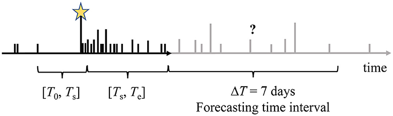
Figure 1. Illustration of the temporal structure of an earthquake sequence progressing from left to right. The relative heights of the lines indicate the magnitude of the events. The training time interval ranges from [T0, Te]. For ease of interpretation for increasing training time interval durations, Te aligns with the number of days following the mainshock, ΔTm. The training time interval is further divided into the preparatory time interval, [T0, Ts], and target time interval, [Ts, Te]. The mainshock is indicated by the golden star. Forecasting takes place during a ΔT = 7 days period immediately following the training time interval.
The two competing aftershock models can be fitted to the aftershock sequence with increasing ΔTm using the maximum likelihood estimate (MLE) method to estimate the aftershock rate model parameters ω, for both the ETAS model and MOL, and the GR law parameter θ [47–49]. The MLE produces point parameter estimates based on the training time interval by maximizing the log-likelihood function. The likelihood is the probability of observing the aftershocks within the training time period given the model [44]. For any time dependent point process model with a well-defined intensity function (e.g., Equations 1 and 2), the likelihood function is
where is the probability density function and is the productivity of the process during the time interval [Ts, Te] having Ne number of events above a specified magnitude. Its derivation can be found in [44, 50].
The log-likelihood is maximized using all events within the target time interval above m0 and above the maximum depth for the sequence. For binned magnitudes, as is the case with earthquake catalog data, θ can be solved using the MLE method for magnitudes exceeding m0 [47–49].
Using the parameter point estimates from the MLE as prior information, MCMC sampling is applied to the same training time intervals to produce model parameter distributions. The sampling procedure accounts for the uncertainty in the model parameter estimates and uses Bayesian methods to incorporate prior knowledge from the MLE estimates [36, 37, 51].
The MCMC method in this study uses the Metropolis-Hastings algorithm for the MOL and Metropolis-within-Gibbs sampling algorithm for the ETAS model to sample the posterior distributions of the model parameters. The detailed description of the implemented algorithms are given in [37]. The posterior distribution is described by
p(θ, ω|S) provides constraints on the model parameter variability by using prior information π(θ, ω) and information obtained from the training data via the likelihood function L(S|θ, ω).
In this study, we use the Gamma distribution as the prior distribution for the model parameters [37]. This choice of the priors is dictated by the well-defined functional form of the Gamma distribution that allows to limit the parameter values in certain ranges which are inferred from past studies. The Gamma distribution is described by its mean and variance, where θ and ω from the MLE are used as the mean for the Gamma priors. Use of other priors was discussed in [37]. The proposal distributions used in the MCMC sampling are set so that the parameters are chosen to approximate the posterior distribution [37]. These are the multi-variate lognormal distribution for both models. The first 100,000 steps are discarded for “burn-in” and 100,000 steps are sampled for the parameter estimates so the distribution only represents the latter 100,000 steps. Each of the resulting 100,000 model parameter estimates are then used for the forward simulations. The full details of the implementation of the Metropolis-within-Gibbs algorithm can be found in [37].
2.4. Magnitude of completeness
To properly estimate the aftershock rate and model parameters, the impacts of early aftershock incompleteness need to be considered [17, 52–56]. If many of these smaller events are missing from the catalog when training, this may result in bias during the subsequent aftershock rate analysis. We identify the magnitude completeness of the sequence by plotting the first 3 days of the sequence on a log-log plot using visual inspection. We then select a magnitude cutoff, m0, where all events ≥ m0 are included in the analyses. It is also important not to select too high a value for m0 as doing so reduces the amount of data available for training. In particular, the ETAS model tends to underestimate the number of events during a forecast when selecting higher m0 and the productivity from small events is not accounted for [57].
2.5. Forecasting with the Bayesian predictive distribution
The forecasting time interval, [Te, Te + ΔT], immediately follows the training time interval. The parameter estimates from the training time interval are used to simulate and forecast events during the forecasting time interval. In this work, the length of the forecasting time interval was set to 7 days, ΔT = 7 days (Figure 1). The simulation of the MOL and ETAS models during the forecasting time interval is performed using the thinning algorithm [58]. For the ETAS model all observed earthquakes prior to the forecasting time intervals are used to properly define the rate during the forecasting time interval.
The point parameter estimates for the MOL and the GR law model parameter from the MLE can be directly used to calculate the probability of the largest events during the forecasting time period by means of the extreme value theory (EVD method) [37]. The probability of a large aftershock during ΔT is PEV. This method is equivalent to the Reasenberg-Jones method [59]. For the productivity , PEV can be calculated as [37]:
where mex is the magnitude of the events that we are forecasting for. To incorporate the uncertainty in the model parameter estimates, we use the Bayesian predictive distribution (BPD) [36, 37, 60]:
To compute the BPD, MCMC sampling of the posterior distribution p(θ, ω|S) of the model parameters are generated during the training time interval and are used to forward simulate the sequence in time as an ensemble during the forecasting time interval, ΔT. The simulations are used to compute the probability of large aftershocks during ΔT.
2.6. Forecast performance testing
The forecast generates earthquake rates in bins for a range of magnitudes and time intervals [35]. The number of predicted events in each bin is calculated from the rate. The expectations can then be produced by assuming the probability of observing events in each bin follows the Poisson model. The joint log-likelihood is the sum of all the logs of the likelihoods in each bin when comparing the expectation to the observed events in each bin as formulated by [9]. This forms the basis of the likelihood tests.
In this work, the forecasts tests are consider the number test (N-test) and magnitude test (M-test) to evaluate these aspects individually. Two comparative tests, the ratio test (R-test) and T-test are applied to assess the relative performance of the forecasts [10, 34]. These tests are based on the assumption that the events are Poisson distributed and use a simple Poisson based likelihood function. This differs from the definition of the likelihood used in the formulation of the ETAS model, Equation (6) [19]. As a result, this may introduce confounding effects when applied to forecasts produced by the ETAS model. In addition, the Bayesian p-test is used to evaluate the performance of the BPD [36]. The first four were adapted from tests used by the Collaboratory for the Study of Earthquake Predictability (CSEP) and follow the same assumptions where the magnitudes are binned and the number of earthquakes in each forecast bin are Poisson-distributed and independent of each other [9, 35, 61]. The effective significance level of 5% for all the tests are used following [62]. Quantile scores exceeding the significance level are considered a passing score on the test. However, the applicability of the CSEP framework to the ETAS model can be considered approximate, because the ETAS model deviates from the Poisson assumption placed on the occurrence of events in the CSEP framework [19–23].
The N-test compares the number of events simulated during the forecasted time period to the number of observed events during the same time period [9]. There is an associated quantile score considered for the N-test, δ. The quantile score indicates if the generated sequences produced forecasted event numbers Ni, i = 1, ..., Nsim, above or below the observed values Nobs. In this work, the estimation of the quantile is performed through simulations of the respective point processes [9, 35]
where Nsim is the total number of simulations and I(x) is the indicator function. A value of δ close to 1 indicates that the forecast underpredicts the observed number of events, and a small δ indicates that the forecast overpredicts the observed number of events. Thus, if the probability of δ is smaller than the half of the significance level αq/2 or larger than 1 − αq/2, the forecast can be rejected [9]. The significance level for the respective N-tests is set to 5% (αq = 0.05) [9].
The M-test evaluates the distribution of the magnitudes of the forecasted events during the forecasting time period compared to the true magnitude distribution of the observed events [9, 35]. For this test, the magnitude distribution is conditioned on the number of forecasted events by considering the forecasts such that the number of simulated events Ni = Nobs. The testing is done by computing the joint log-likelihood score of the simulated magnitude events. The M-test statistic is indicated by the κ as shown in
where Mobs is the joint log-likelihood of the observed events and Miis the joint log-likelihood computed for every simulation i = 1, ..., Nsim [9].
The R-test compares two different forecasting models relative to each other by assuming one of the models is true and stands in as the null hypothesis, which is referred to as the reference hypothesis H2. The competing model hypothesis is H1. Each of the models has a likelihood score from the L-test based on the modified observed events assuming the null hypothesis is true (H2 corresponds with likelihood score L2 and H1 corresponds with likelihood score L1). The L-test formulation and details can be found in [35, 36]. The R-test provides the ratio of the likelihoods for two models R21, where R21 = L2 − L1 [35]. If R21 > 0, then the reference model H2 performs better. Similarly, a larger quantile score for the R-test, the quantile score α, indicates that H2 performs better than H1. The definition of the quantile score α is given in [10]. This test is reversible, and the null hypotheses can be set as the other model. If both models when set as the reference hypotheses result in a quantile score α larger than the effective significance level, then neither model can be rejected using the R-test [10].
To provide additional context for the R-test and to reduce computational time, the T-test, inspired by Student's t-test, was introduced as a proxy for the R-test [10]. The results of the T-test indicate whether a competing hypothesis has performed better than or is inconsistent with the reference hypothesis by evaluating the significance of the information gain. The T-test score results in the sample information gain of one model over another, where the sample information gain from the reference hypothesis (H2) over the alternate hypothesis (H1) is shown as IG(H2, H1) for Nobs, the number of observed events during the forecasting time interval ΔT [10]:
Positive values demonstrate information gain, where information gain IG > 1 can be considered significant. Negative values on the T-test indicate that the alternative hypothesis performs better than the reference hypothesis. As with the R-test, the T-test can also be reversed by changing the reference and alternative hypotheses to investigate the information gain in the other direction.
For forecasts that use the BPD method to generate probabilities, the Bayesian p-test (herein p-test) can be conducted. The value pB gives the probability that the largest event in the simulations for the forecasted sequence will be more extreme than the observed largest event during the forecasting time interval. pB is described as [36]:
The p-test has a test quantity (t, θ, ω) for the observed variable y and the simulated quantity ŷ. In this case, maxy is the largest event in the simulation, and pB is the proportion of the test quantities from the simulated maximum events that are greater than or equal to the observed largest event during the forecasting time interval. Extreme values of pB ≈ 0 indicate that the features are not well demonstrated by the model [36].
2.7. Aftershock sequences
The evaluated sequences include the 2009 L'Aquila (LAQ), Italy; 2010 Darfield (DFL), New Zealand; 2016 Amatrice-Norcia (AMA), Italy; 2016 Kumamoto (KUM), Japan; and 2020 Monte Cristo Range (MCR), United States of America. The mainshock magnitudes and dates are presented in Table 1. The spatial distributions of the epicenters of earthquakes for each sequence are given in Supplementary Figures 1–5 as indicated by the dashed ellipses. A brief description of the sequence conditions are as follows. The 2009 L'Aquila (LAQ) sequence began in the central Apennines next to large and normal faults [64]. In the months leading up to the LAQ sequence, there was increased background seismicity [65]. The 2016 Amatrice-Norcia (AMA) sequence took place in central Italy, which activated a 60 km normal fault system [66]. This sequence was evaluated independently of the LAQ sequence, though it is worth noting the aftershocks from the LAQ sequence appeared to migrate toward the AMA sequence region. The catalogs for the LAQ and AMA sequence were retrieved from the Italian Seismological Instrumental and Parametric Database.
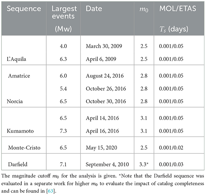
Table 1. List of analyzed sequences including the date of the initiating event for the sequence in UTC and the magnitude of the largest event.
The 2016 Kumamoto (KUM) sequence began with a foreshock sequence before the mainshock of Mw 7.3. The events of the sequence indicated a right lateral strike-slip fault along the Futagawa fault segment [67]. The catalog for this sequence was retrieved from the Japan Meteorological Agency catalog. The Monte-Cristo (MCR) sequence took place along a previously unmapped, steeply dipping fault near Walker Lane, Nevada. The aftershocks took place with a mix of left-lateral, right-lateral, and normal fault motions [68]. The catalog for the MCR sequence was retrieved from the United States Geological Survey Advanced National Seismic System Comprehensive Earthquake Catalog. The 2010 Darfield (DFL) sequence took place on previously unmapped faults, in association with strike-slip movement with a reverse component for the mainshock [69, 70]. The catalog for the DFL sequence was retrieved from GeoNet.
3. Results
Results of the forecasting test performance for the five selected sequences for their respective training time intervals are presented in this section. We first show the forecasts that are generated using the BPD and provide general interpretations without the performance metrics. Then the N- and M-test results are presented together as part of the classic likelihood L-test. We also use the Bayesian p-test that demonstrates the performance of the BPD forecasting method. The comparative R- and T-tests are then presented together to evaluate the relative performance of the forecasts. For further details, the performance of the individual sequences is provided in Section 3.4.
3.1. Maximum likelihood estimates and forecasts
The forecasts that are being evaluated are generated using the BPD method after an initial model parameter estimation using the MLE, which are used as prior distributions for the model parameters. Here we use the LAQ sequence as an example. The model parameter estimates using the MLE are provided in Supplementary Figures 10–14 for all of the five sequences and training time intervals. Reviewing the MLE estimates, it can be observed that the model parameters tend to stabilize and converge with increased ΔTm, generally stabilizing after ΔTm = 3 days for all of the sequences and aftershock models (Supplementary Figures 10–14).
The forecast can be produced for both models using the BPD method by MCMC sampling of the posterior distributions and forward simulating the models during the forecasting time interval. Plots indicating the probability of the largest expected event ≥ mex during the forecasting time interval ΔT = 7 days are shown for each training time interval in Figure 2 for the 2009 L'Aquila sequence and in Supplementary Figures 6–9 for the rest of the sequences. The end of each training time interval Te corresponds with the number of days following the mainshock ΔTm. We considered ΔTm = [1, 2, 3, 4, 5, 6, 7, 10, 14, 21, 30] days for the training time intervals. Overall, the probability for the largest expected events decreases as the training time interval increases. Slight increases in probability are aligned with changes in the model parameter estimates for rate and decay parameters. For example, in the LAQ sequence, the model parameter K for the ETAS model jumps from 0.74 to 16.05 and p decreases from 3.2 to 2.2. There is a clear increase in probability for this training time interval and the increased rate outweighs the decrease in productivity α. The probability for an event with magnitude ≥ mex increases following ΔTm = 3 days. This increase is accompanied by a decrease in decay rate (increase in p) and increase in productivity parameter α. The observed seismicity rate can be seen in the density of the black open diamonds in Figure 2. The spike in the MOL forecast for the LAQ sequence follows a slight delay that is reflected in the adjustment of the decay rate po.
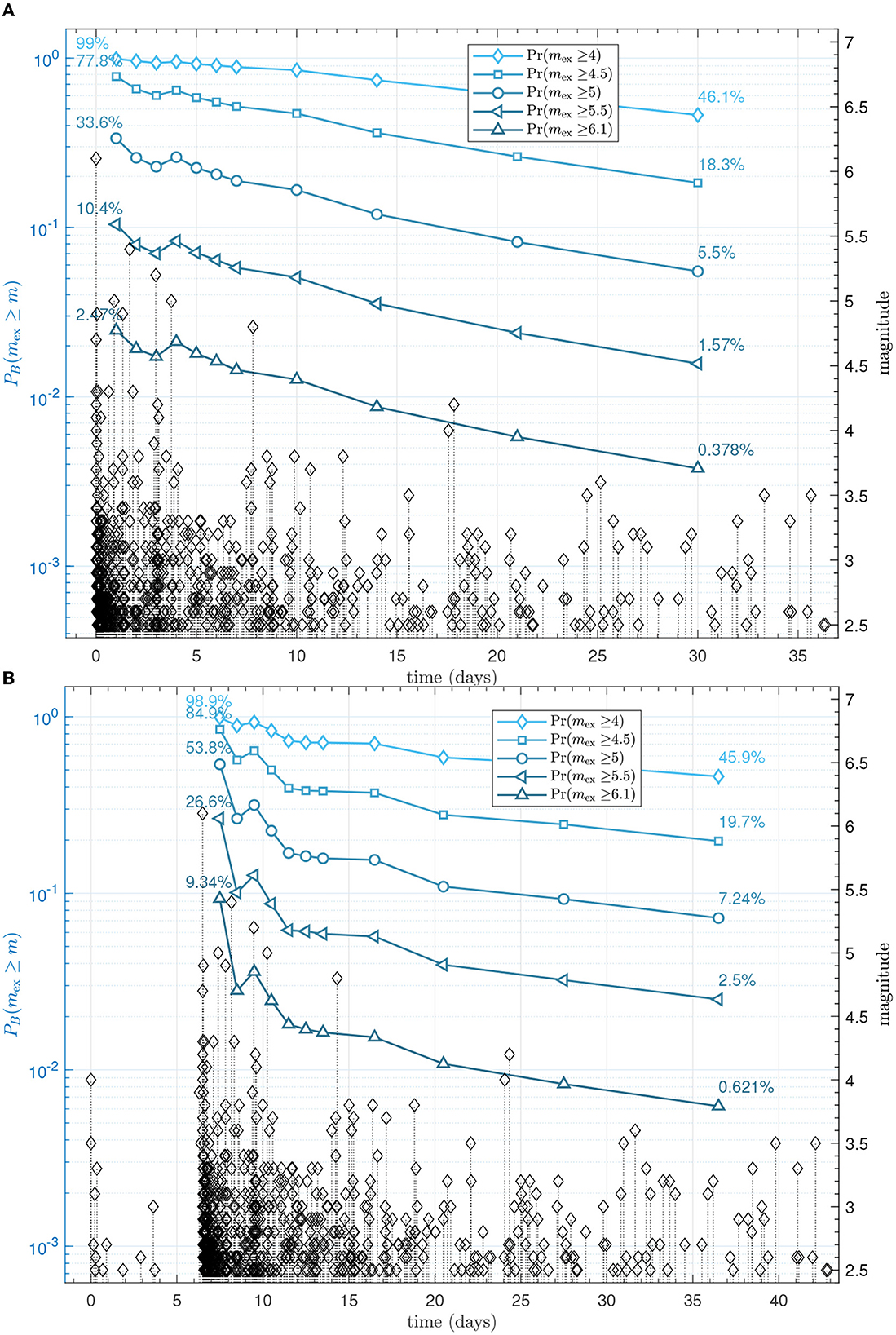
Figure 2. Forecasted probabilities for the occurrence of the largest expected aftershocks to be above mex ≥ [4.0, 4.5, 5.0, 5.5, 6.1] during the forecasting time interval ΔT = 7 days for the 2009 L'Aquila sequence. Time ΔTm indicates the number of days from the April 6, 2009 mainshock. (A) Indicates the forecasting probability when using the MOL model; (B) Indicates the forecasting probability when using the ETAS model. Additional data prior to the mainshock is also shown, as these events were used as part of the ETAS model.
It can be observed that the increased probability in the ETAS model aligns well with the local cluster of high density observed events following ΔTm = 3 days, whereas the MOL peak probability for large events occurs after this cluster. This is expected, as MOL does not account for potential clustering during the forecast and incorporates the increased seismicity only after it takes place. In addition, when considering all of the sequences and their forecasts, the probability of large aftershock increases more for the ETAS model than the MOL following a large aftershock that is associated with an increase in the seismicity rate during the training time interval. The probability of large aftershocks decreases following the mainshock in general.
3.2. Likelihood tests and Bayesian pB-value
The N-test applied to the sequences indicates that the number of events is typically overestimated for all training time intervals for the ETAS model as indicated by the low δ scores for the DFL and AMA, and MCR sequences (Figure 3). The number of events for the MOL forecasts alternates between over- and underestimation of the observed number of events. The plots of the forecasted and observed number of events for all five sequences are given in Supplementary Figures 15–19. From the N-test plots, the effective significance score is not consistently passed on both sides for most training time intervals for both aftershock rate models. The overestimation of the MOL can be directly related with the model parameter Ko, which is larger when the rate is overestimated, or with the po estimate, when it is small and the rate of aftershock decay is slow (Supplementary Figures 10–14). The ETAS model overestimation cannot be directly related to a single model parameter. For most of the sequences, the background seismicity was very low and could not be the primary contributor to the overestimation from the ETAS model with the exception of the KUM sequence which had relatively high background seismicity estimates.
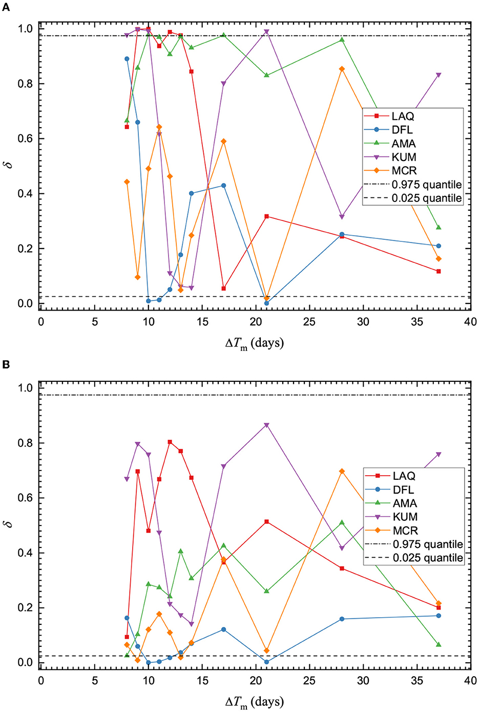
Figure 3. Quantile score δ for the N-test for all of the evaluated sequences. Horizontal lines are drawn for quantile scores of 0.025 and 0.975. The score is plotted to correspond with the end of each forecasting time interval. Plot (A) shows the MOL performance while plot (B) shows the ETAS quantile scores. The corresponding forecasted numbers of events are given in Supplementary Figures 15–19.
The MOL aftershock rate is not affected by the GR law. However, for the ETAS model, it is important to consider whether the events are impacted by the magnitude distribution from which the model draws from. For the M-test, it can be observed that when the number of events forecasted is scaled to the observed events, the magnitude distribution of the forecast closely represents the observed magnitude distribution (Figure 4). This is not surprising as this is isolated from the aftershock rate models. The impact of the GR law can be interpreted to be minimal on the number of forecasted events for the ETAS model. The MOL aftershock rate and number of events during the forecast are not impacted by the GR law. From the M-test scores, the ETAS model performance can be considered reliable and independent of the impact of the GR law fitting.
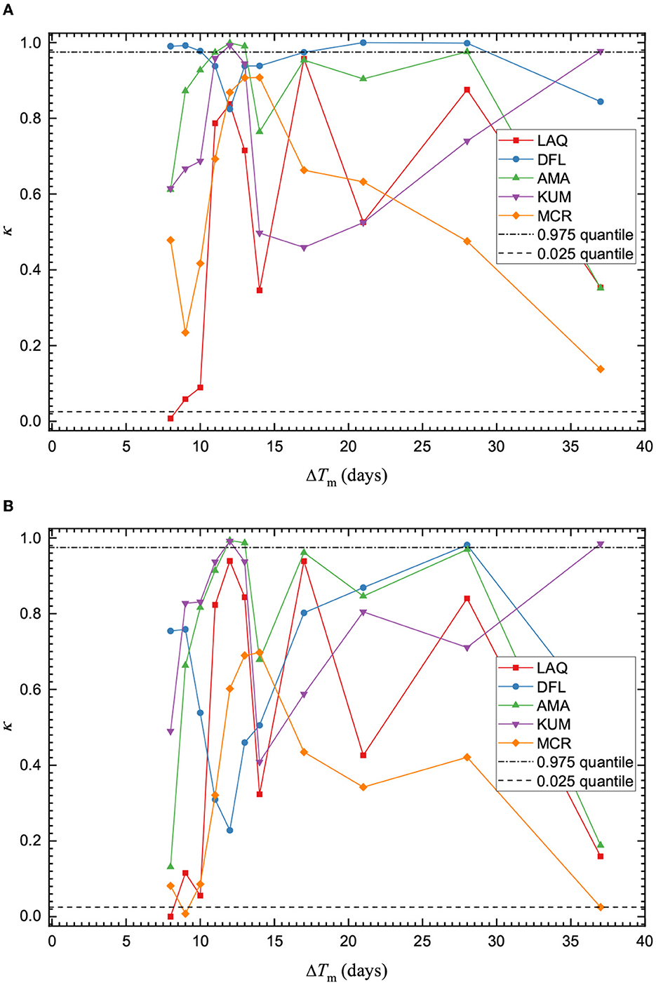
Figure 4. Quantile scores κ of the M-test for the (A) MOL and (B) ETAS model. Horizontal lines are drawn for quantile scores of 0.025 and 0.975. The score is plotted at the end of each forecasting interval. Overall, the M-test performance is similar for both aftershock models.
It can be observed that the performance of the MOL on the M-test typically results in a larger quantile score than the ETAS model. However, it does mimic the same trends as observed for the ETAS model. For the MOL, the training time interval is slightly longer. This suggests that the magnitude distribution immediately following the mainshock strongly influences the performance of the M-test and does not represent the magnitude distribution of events well. It follows that the b-value may be better estimated when the effect of the mainshock and in the immediate surrounding are minimized.
Both models perform well on the Bayesian p-test, except for the DFL sequence, suggesting that both models sufficiently captured the probability of the largest observed event in the forecast, so neither was rejected (Figure 5). This confirms the procedure is suitable for providing a forecast.
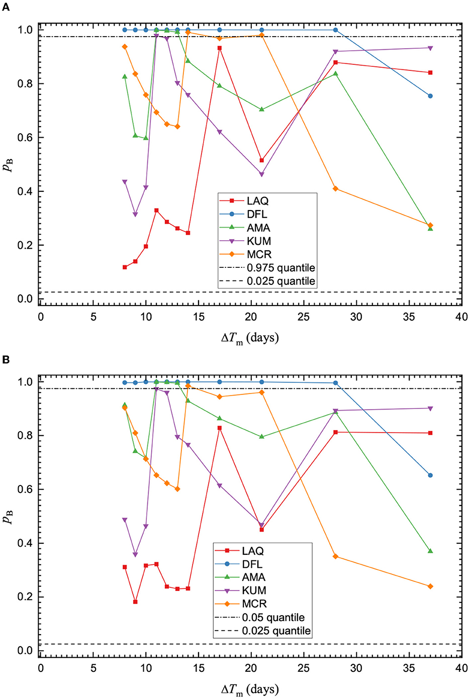
Figure 5. Quantile scores for the Bayesian p-test are shown for the (A) MOL and (B) ETAS models. Horizontal lines are drawn for quantile scores of 0.025 and 0.975. The score is plotted at the end of the training time interval ΔTm and is evaluated for a forecasting time interval of ΔT = 7 days. Most training time intervals for both models typically pass the p-test. The scores are similar for the respective aftershock models.
3.3. Model forecast comparison tests
When comparing the performance of the two aftershock models directly, the R-test demonstrates that it is possible for both sides of the test to be passed or failed regardless of the reference model [10]. However, we find that the MOL is more likely to be rejected as an alternative hypothesis when the ETAS model is considered the reference model (Figure 6). This suggests that the MOL model tends to perform better than the ETAS model for the selected training time intervals and sequences. This is supported by the results of the T-test. The information gain of the MOL when the ETAS model is the reference model is typically negative, indicating a loss of information (Figure 7).
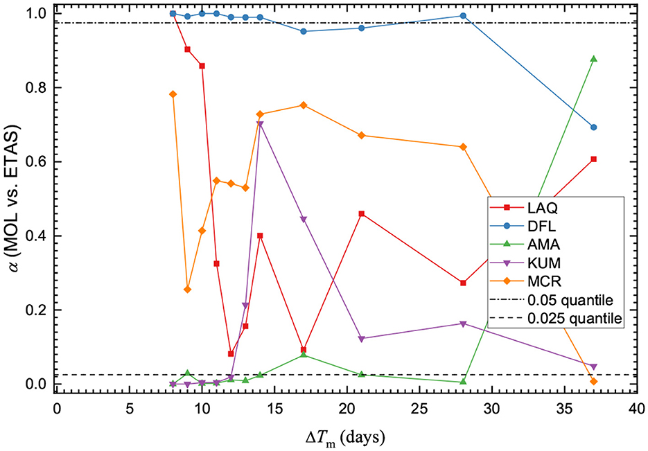
Figure 6. Quantile scores α for the R-test when the MOL is set as the hypothesis H1 and the ETAS model is set as the hypothesis H2. Horizontal lines are drawn for quantile scores of 0.025 and 0.975. The score is plotted at the end of the training time interval ΔTm and is evaluated for a forecasting time interval of ΔT = 7 days.
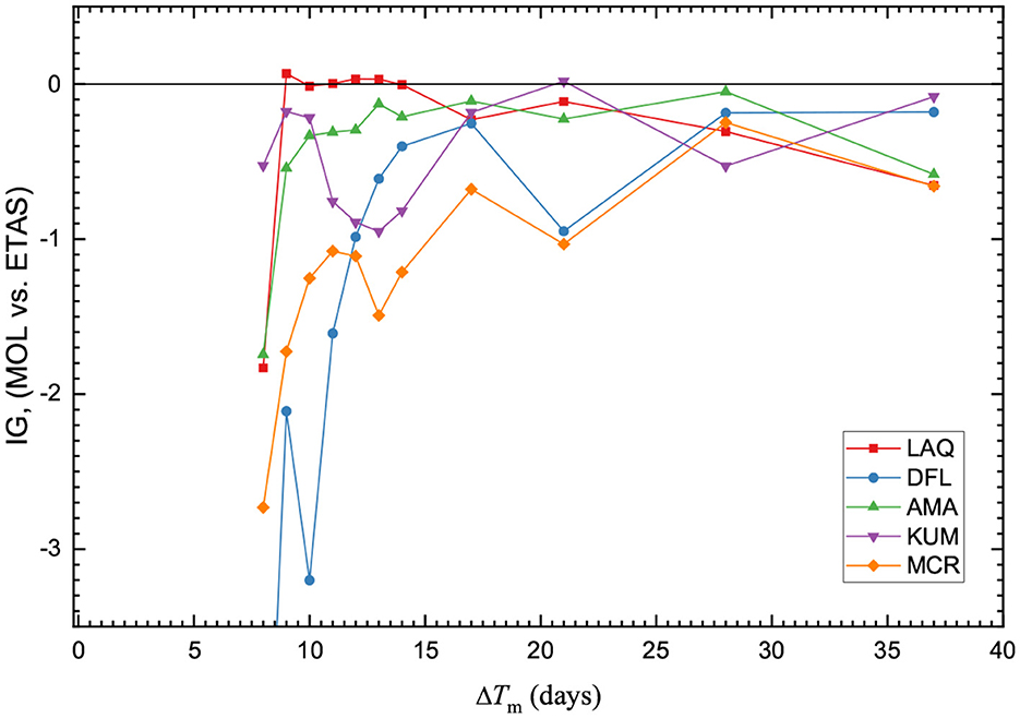
Figure 7. Information gain IG(H2, H1) for the respective sequences when the MOL is set as the hypothesis H1 and the ETAS model is set as the hypothesis H2. A horizontal line is drawn at IG = 0. The score is plotted at the end of the training time interval ΔTm and is evaluated for a forecasting time interval of ΔT = 7 days.
3.4. Performance on statistical tests for specific sequences
The 2009 L'Aquila sequence had a large aftershock of M = 5.4 2 days following the mainshock. The ETAS model reflected the increase in seismicity and corresponding large aftershock probability before the occurrence of the large aftershock (Figure 2). The ETAS model starts to overestimate the number of events after ΔTm = 7 days (Supplementary Figure 15B). The MOL underestimates the number of forecasted events earlier in the sequence (Supplementary Figure 15A). This corresponds with a decline on the M-test performance for both aftershock rate models, which suggests that the ETAS underestimation was influenced by the magnitude distribution, while the MOL independently underestimated the number of forecasted events. In contrast to [71], the ETAS model performed comparably to the MOL based on the T-test for most of the training time intervals.
The 2010 Darfield sequence was less seismically active than would be expected based on the New Zealand aftershock decay model [72]. Previous work has shown that the ETAS model performs better than the regional models using the 3 month and 1 day forecast of the sequence [73]. On the N-test, the number of events forecasted during the simulations is overestimated by the ETAS model for the various training time intervals (Supplementary Figure 16B). The MOL fluctuates between over- and underestimation of the observed events during the forecast simulations, though the number of forecasted events is closer to the observed events for longer training time intervals ΔTm ≥ 10 days (Supplementary Figure 16A). The performance on this test also impacts the results of the p-test. For extremely high values on the p-test, where pB ≈ 1, we can observe that the number of events on the N-test was overestimated at these time intervals. On the M-test, the magnitude distributions of the two aftershock models paralleled each other and performed well, with quantile scores above the effective significance level (Figure 4).
The 2016 Kumamoto sequence is an example of a foreshock sequence with a typical aftershock sequence following the mainshock. The ETAS model was fitted in such a way to include the foreshock sequence during the model parameter estimations. The MOL was limited to data following the mainshock. Both models stabilized around the same training time interval length. However, the MOL underestimated the number of forecasted events during the first four training time intervals following the mainshock (Supplementary Figure 17A). This is unsurprising as decay of the foreshock sequence may have continued to contribute to the seismicity and could not be explicitly accounted for using the MOL. The ETAS model tended to slightly overestimate the number of events, which partly corresponds to the high background seismicity estimates (Supplementary Figure 17B). The M-test was passed by both models for all training time intervals. Comparison of the two models on the T-test indicate that the MOL model consistently demonstrates small information gain over the ETAS. We note that the model parameters for the KUM sequence show a distinct shift in the estimated background seismicity around ΔTm = 7 days, which may contribute to the observed features (Supplementary Figure 12). Despite the estimation of a high background rate, the performance on the N-test indicated that the ETAS model alternated between over- and under-estimation of the number of events during the forecasting time interval. When evaluating the forecasting scores for ΔTm ≥ 10 days, then the ETAS model performs slightly better than the MOL.
The 2016 Norcia sequence is an example of a classic foreshock–aftershock sequence. The background seismicity of the sequence was considered elevated due to the occurrence of the Mw 6.0 Amatrice mainshock on August 24, 2016, and set to μ = 1.0. It can be observed that the MOL model parameters are stable and estimated consistently during all of the training time intervals (Supplementary Figure 13A). The ETAS model parameters stabilize following ΔTm = 4 days (Supplementary Figure 13B). The ETAS model forecast tended to overestimate the number of events in the forecasting time interval, though not greatly (Supplementary Figure 18B). The MOL tended to underestimate the number of events during the forecasting time interval (Supplementary Figure 18A). In the comparison tests, the MOL model consistently demonstrated information gain over the ETAS and the R-test was failed by the MOL in several instances which agrees with [66].
The 2020 Monte Cristo Range sequence demonstrates an example of multiple ETAS model parameters being constrained to produce consistent estimates. The MOL parameters converged after ΔTm = 3 days, with the Ko parameter remaining consistent (Supplementary Figure 14). The performance on the N- and M-test are similar, though the MOL performs better on the N-test by more frequently scoring a pass on both sides of the test. The ETAS model typically overestimates the number of forecasted events (Supplementary Figure 19B). The MOL model demonstrates marginal information gain over the ETAS model. For this sequence, while the MOL model appears to perform better than the ETAS model, it is not fully clear if the improvement is significant.
4. Discussion
In this paper, we fitted the ETAS model and MOL to different earthquake sequences and evaluated their forecasting performance from the BPD method using five statistical tests. From the tests, we evaluated the quantitative scores for the likelihoods and relative performance of the forecasts. From previous work in [63], we also found that an increase in the magnitude cutoff used for analysis did not change the general interpretation of the forecast tests, implying that the tests can be applied to catalogs with higher magnitude of completeness.
We observed that for most of the sequences, the early performance on the T-test was indicative of the performance on the T-test for longer training time intervals. When the T-test score is either positive or negative during the first few training time intervals, it appears likely that the score remains positive or negative.
We found that the forecast produced by the ETAS model does typically perform well on most of the tests. However, the information gain of the ETAS model over the MOL was not consistent for all sequences and the choice of the ETAS model for operational forecasting should be done with caution. One possible explanation is related to the fact that the fitting of the ETAS model typically requires more data points to achieve reasonable convergence compared to the MOL model. However, due to the early incompleteness of the aftershock sequences one has to use higher magnitude cutoffs to ensure that the sequence is complete. This reduces the number of events and results in large uncertainties in the estimated parameters of the ETAS model.
With respect to the information gain, it can be observed that the N-test does not appear to be a good predictor of the T-test (Figures 3, 7). Instead, the quantile scores for the N-test tend to swing to one extreme or another (over/underestimation). Thus, the N-test is not sufficient to determine which model provides a better forecast. The quantile scores of the N-test are more useful to determine the overall behavior of the forecast and aftershock model based on the forecasting time interval than for direct comparison of different aftershock models for these sequences.
The performance on the R-test in Figure 6 was generally consistent for all of the sequences that were evaluated in this study and was not found to be a useful test when choosing a better performing aftershock model. The performance of the MOL and ETAS model for the M-and p-tests in Figures 4, 5 was unsurprising, as the results are more reflective of the estimated b-values rather than the model rate parameters ω. To better isolate the impact of the aftershock models, a generic b-value with a wider distribution rather than Gamma prior based on the MLE estimate and user selected variance can be used. In addition, high quantile scores on the N-test for the δ score were also reflected in the p-test. As the p-test is not scaled to the number of observed events, it is easy to perform well on the p-test if the number of aftershocks is overestimated.
We highlighted the importance of conducting multiple tests and noted the specific impacts of model parameter estimates on the performance scores. We also demonstrated the necessity of conducting the comparative tests in addition to the likelihood tests, as the interpretation from the N-test results would have suggested that the MOL typically performs better than the ETAS model. The most practical outcome of this study is the implication that information gains when evaluating competing aftershock rate models for longer training time intervals can be inferred by early training time intervals. Specific constraints on this generalization can be further evaluated for practical applications.
The results of this work suggest a caution when using the ETAS model as the preferred model for forecasting. As the ETAS model forecast is computationally expensive and time consuming to produce in real-time, it is recommended that the MOL forecast is used as the baseline probability. While the ETAS appears to perform better on the comparative tests, the information gain is not sufficiently large enough to discount the MOL as a suitable model for forecasting. In addition, the tests based on the Poisson assumption are not fully applicable to the ETAS model as it deviates from the Poisson statistics [19–23].
Several additional assumptions were made with this work. The first is that the aftershock magnitudes can be represented by the b-value estimated from the training time intervals. The second is that there is no evolution in the background seismicity during the sequence. These assumptions impact the ETAS model disproportionately as the rate is dependent on both of these model parameters, whereas the MOL rate during the observation is independent of these parameters.
An additional limitation addressed in a previous work by [37], is the forecasting time intervals. The forecasting in this work was limited to using 7 days as the forecasting time interval, which is a reasonable representation of the forecasting time interval that would be considered for real-time forecasting. On the other hand, longer time intervals may favor the ETAS model as it takes into account the occurrence of secondary aftershock sequences.
Data availability statement
Publicly available datasets were analyzed in this study. The earthquake catalogs were obtained from the following databases: the Japan Meteorological Agency (http://www.jma.go.jp/en/quake/); U.S.G.S. Composite Catalog (https://earthquake.usgs.gov/earthquakes/search/); New Zealand GEONET (http://quakesearch.geonet.org.nz/); the Italian Seismological Instrumental and Parametric Database (http://terremoti.ingv.it/en/search).
Author contributions
ED performed the research, analyzed the data, and wrote the manuscript. RS formulated the problem, supervised the research, wrote the computer codes, contributed to the writing of the manuscript, and handled the manuscript submission to the journal. KG supervised the research, contributed to data analysis, and the writing of the manuscript. All authors contributed to the article and approved the submitted version.
Funding
This work has been supported by the NSERC Discovery grant and by NSERC Create grant.
Acknowledgments
We would like to thank Yicun Guo and David Harte for their constructive and helpful critique of the manuscript that helped to improve the presentation and clarify results.
Conflict of interest
The authors declare that the research was conducted in the absence of any commercial or financial relationships that could be construed as a potential conflict of interest.
Publisher's note
All claims expressed in this article are solely those of the authors and do not necessarily represent those of their affiliated organizations, or those of the publisher, the editors and the reviewers. Any product that may be evaluated in this article, or claim that may be made by its manufacturer, is not guaranteed or endorsed by the publisher.
Supplementary material
The Supplementary Material for this article can be found online at: https://www.frontiersin.org/articles/10.3389/fams.2023.1126511/full#supplementary-material
References
1. Kossobokov VG. Earthquake prediction: 20 years of global experiment. Nat Hazards. (2013) 69:1155–77. doi: 10.1007/s11069-012-0198-1
2. Zhang L, Werner MJ, Goda K. Spatiotemporal seismic hazard and risk assessment of aftershocks of m 9 megathrust earthquakes. Bull Seismol Soc Am. (2018) 108:3313–35. doi: 10.1785/0120180126
4. Shcherbakov R, Turcotte DL. A modified form of Båth's law. Bull Seismol Soc Am. (2004) 94:1968–75. doi: 10.1785/012003162
5. Shcherbakov R, Goda K, Ivanian A, Atkinson GM. Aftershock statistics of major subduction earthquakes. Bull Seismol Soc Am. (2013) 103:3222–34. doi: 10.1785/0120120337
7. Utsu T. Aftershocks and earthquake statistics (ii) further investigation of aftershocks and other earthquake sequences based on a new classification of earthquake sequences. J Facul Sci. (1971) 3:197–266.
8. Shcherbakov R, Turcotte DL, Rundle JB, Tiampo KF, Holliday JR. Forecasting the locations of future large earthquakes: an analysis and verification. Pure Appl Geophys. (2010) 167:743–9. doi: 10.1007/s00024-010-0069-1
9. Zechar JD, Gerstenberger MC, Rhoades DA. Likelihood-based tests for evaluating space-rate-magnitude earthquake forecasts. Bull Seismol Soc Am. (2010) 100:1184–95. doi: 10.1785/0120090192
10. Rhoades DA, Schorlemmer D, Gerstenberger MC, Christophersen A, Zechar JD, Imoto M. Efficient testing of earthquake forecasting models. Acta Geophys. (2011) 59:728–47. doi: 10.2478/s11600-011-0013-5
11. Page MT, van der Elst N, Hardebeck J, Felzer K, Michael AJ. Three ingredients for improved global aftershock forecasts: tectonic region, time-dependent catalog incompleteness, and intersequence variability. Bull Seismol Soc Am. (2016) 106:2290–301. doi: 10.1785/0120160073
12. Hardebeck JL, Llenos AL, Michael AJ, Page MT, van der Elst N. Updated California aftershock parameters. Seismol Res Lett. (2019) 90:262–70. doi: 10.1785/0220180240
13. Omi T, Ogata Y, Shiomi K, Enescu B, Sawazaki K, Aihara K. Implementation of a real-time system for automatic aftershock forecasting in Japan. Seismol Res Lett. (2019) 90:242–50. doi: 10.1785/0220180213
14. Marzocchi W, Lombardi AM. Real-time forecasting following a damaging earthquake. Geophys Res Lett. (2009) 36:L21302. doi: 10.1029/2009gl040233
15. Omi T, Ogata Y, Shiomi K, Enescu B, Sawazaki K, Aihara K. Automatic aftershock forecasting: a test using real-time seismicity data in Japan. Bull Seismol Soc Am. (2016) 106:2450–8. doi: 10.1785/0120160100
16. Ogata Y, Katsura K. Point-process models with linearly parametrized intensity for application to earthquake data. J Appl Prob. (1986) 23:291–310. doi: 10.2307/3214359
17. Ogata Y. Statistical-models for earthquake occurrences and residual analysis for point-processes. J Am Stat Assoc. (1988) 83:9–27.
18. Zhuang J. Next-day earthquake forecasts for the Japan region generated by the ETAS model. Earth Planets Space. (2011) 63:207–16. doi: 10.5047/eps.2010.12.010
19. Harte DS. Log-likelihood of earthquake models: evaluation of models and forecasts. Geophys J Int. (2015) 201:711–23. doi: 10.1093/gji/ggu442
20. Harte DS. Model parameter estimation bias induced by earthquake magnitude cut-off. Geophys J Int. (2016) 204:1266–87. doi: 10.1093/gji/ggv524
21. Harte DS. Probability distribution of forecasts based on the ETAS model. Geophys J Int. (2017) 210:90–104. doi: 10.1093/gji/ggx146
22. Harte DS. Effect of sample size on parameter estimates and earthquake forecasts. Geophys J Int. (2018) 214:759–72. doi: 10.1093/gji/ggy150
23. Harte DS. Evaluation of earthquake stochastic models based on their real-time forecasts: a case study of Kaikoura 2016. Geophys J Int. (2019) 217:1894–914. doi: 10.1093/gji/ggz088
25. Dieterich J. A constitutive law for rate of earthquake production and its application to earthquake clustering. J Geophys Res. (1994) 99:2601–18.
26. King GCP, Stein RS, Lin J. Static stress changes and the triggering of earthquakes. Bull Seismol Soc Am. (1994) 84:935–53.
27. Utsu T, Ogata Y, Matsu'ura RS. The centenary of the Omori formula for a decay law of aftershock activity. J Phys Earth. (1995) 43:1–33.
28. Scholz CH. The Mechanics of Earthquakes and Faulting, 2nd Edn. Cambridge: Cambridge University Press (2002).
29. Evison FF, Rhoades DA. Demarcation and scaling of long-term seismogenesis. Pure Appl Geophys. (2004) 161:21–45. doi: 10.1007/s00024-003-2435-8
30. Field EH, Dawson TE, Felzer KR, Frankel AD, Gupta V, Jordan TH, et al. Uniform California earthquake rupture forecast, Version 2 (UCERF 2). Bull Seismol Soc Am. (2009) 99:2053–107. doi: 10.1785/0120080049
31. Zhang X, Shcherbakov R. Power-law rheology controls aftershock triggering and decay. Sci Rep. (2016) 6:36668. doi: 10.1038/srep36668
32. Rhoades DA, Christophersen A, Gerstenberger MC. Multiplicative earthquake likelihood models incorporating strain rates. Geophys J Int. (2017) 208:1764–74. doi: 10.1093/GJI/GGW486
33. Strader A, Schneider M, Schorlemmer D. Prospective and retrospective evaluation of five-year earthquake forecast models for California. Geophys J Int. (2017) 211:239–51. doi: 10.1093/GJI/GGX268
34. Kagan YY, Jackson DD. New seismic gap hypothesis: five years after. J Geophys Res. (1995) 100:3943–59. doi: 10.1029/94jb03014
35. Schorlemmer D, Gerstenberger MC, Wiemer S, Jackson DD, Rhoades DA. Earthquake likelihood model testing. Seismol Res Lett. (2007) 78:17–29. doi: 10.1785/gssrl.78.1.17
36. Shcherbakov R. Statistics and forecasting of aftershocks during the 2019 Ridgecrest, California, earthquake sequence. J Geophys Res. (2021) 126:e2020JB020887. doi: 10.1029/2020JB020887
37. Shcherbakov R, Zhuang J, Zöller G, Ogata Y. Forecasting the magnitude of the largest expected earthquake. Nat Commun. (2019) 10:4051. doi: 10.1038/s41467-019-11958-4
38. Ogata Y. Seismicity analysis through point-process modeling: a review. Pure Appl Geophys. (1999) 155:471–507. doi: 10.1007/s000240050275
39. Vere-Jones D. Stochastic models for earthquake sequences. Geophys J Int. (1975) 42:811–26. doi: 10.1111/j.1365-246X.1975.tb05893.x
40. Shcherbakov R, Yakovlev G, Turcotte DL, Rundle JB. Model for the distribution of aftershock interoccurrence times. Phys Rev Lett. (2005) 95:218501. doi: 10.1103/PhysRevLett.95.218501
41. Shcherbakov R, Turcotte DL, Rundle JB. Complexity and earthquakes. In: Kanamori H, editor. Earthquake Seismology, 2nd Edn, Vol. 4. Amsterdam: Elsevier (2015). p. 627–53.
42. Ogata Y. Space-time point-process models for earthquake occurrences. Ann I Stat Math. (1998) 50:379–402.
43. Lombardi AM, Marzocchi W. The ETAS model for daily forecasting of Italian seismicity in the CSEP experiment. Ann Geophys. (2010) 53:155–64. doi: 10.4401/ag-4848
44. Ogata Y. Estimation of the parameters in the modified Omori formula for aftershock frequencies by the maximum-likelihood procedure. J Phys Earth. (1983) 31:115–24. doi: 10.4294/jpe1952.31.115
45. Gutenberg B, Richter CF. Frequency of earthquakes in California. Bull Seismol Soc Am. (1944) 4:185–8.
46. Vere-Jones D. Foundations of statistical seismology. Pure Appl Geophys. (2010) 167:645–53. doi: 10.1007/s00024-010-0079-z
47. Aki K. Maximum likelihood estimate of b in the formula logN = a−bM and its confidence limits. Bull Earthquake Res Inst. (1965) 43:237–9.
48. Utsu T. A method for determining the value of b in a formula logn = a − bM showing the magnitude-frequency relation for earthquakes. Geophys Bull Hokkaido Univ. (1965) 13:99–103.
50. Daley DJ, Vere-Jones D. An Introduction to the Theory of Point Processes, Vol. 1., 2nd Edn. New York, NY: Springer (2003).
51. Shcherbakov R. Bayesian confidence intervals for the magnitude of the largest aftershock. Geophys Res Lett. (2014) 41:6380–8. doi: 10.1002/2014GL061272
52. Kagan YY. Short-term properties of earthquake catalogs and models of earthquake source. Bull Seismol Soc Am. (2004) 94:1207–28. doi: 10.1785/012003098
53. Peng ZG, Vidale JE, Houston H. Anomalous early aftershock decay rate of the 2004 Mw 6.0 Parkfield, California, earthquake. Geophys Res Lett. (2006) 33:L17307. doi: 10.1029/2006GL026744
54. Hainzl S. Rate-dependent incompleteness of earthquake catalogs. Seismol Res Lett. (2016) 87:337–44. doi: 10.1785/0220150211
55. Hainzl S. Apparent triggering function of aftershocks resulting from rate-dependent incompleteness of earthquake catalogs. J Geophys Res. (2016) 121:6499–509. doi: 10.1002/2016jb013319
56. Bhattacharya P, Phan M, Shcherbakov R. Statistical analysis of the 2002 Mw 7.9 Denali earthquake. Bull Seismol Soc Am. (2011) 101:2662–74. doi: 10.1785/0120100336
57. Helmstetter A, Sornette D. Predictability in the epidemic-type aftershock sequence model of interacting triggered seismicity. J Geophys Res. (2003) 108:2482. doi: 10.1029/2003JB002485
58. Zhuang J, Touati S. Stochastic simulation of earthquake catalogs. In: Community Online Resource for Statistical Seismicity Analysis (2015). doi: 10.5078/corssa-43806322
59. Reasenberg PA, Jones LM. Earthquake hazard after a mainshock in California. Science. (1989) 243:1173–6. doi: 10.1126/science.243.4895.1173
60. Shcherbakov R, Zhuang J, Ogata Y. Constraining the magnitude of the largest event in a foreshock-mainshock-aftershock sequence. Geophys J Int. (2018) 212:1–13. doi: 10.1093/gji/ggx407
61. Zechar JD, Jordan TH. Testing alarm-based earthquake predictions. Geophys J Int. (2008) 172:715–24. doi: 10.1111/j.1365-246X.2007.03676.x
62. Taroni M, Marzocchi W, Schorlemmer D, Werner MJ, Wiemer S, Zechar JD, et al. Prospective CSEP evaluation of 1-day, 3-month, and 5-yr earthquake forecasts for Italy. Seismol Res Lett. (2018) 89:1251–61. doi: 10.1785/0220180031
63. Dong E. Testing aftershock forecasts using Bayesian methods (Electronic thesis). The University of Western Ontario, London, ON, Canada (2022).
64. Woessner J, Laurentiu D, Giardini D, Crowley H, Cotton F, Grünthal G, et al. The 2013 European seismic hazard model: key components and results. Bull Earthquake Eng. (2015) 13:3553–96. doi: 10.1007/S10518-015-9795-1
65. Papadopoulos GA, Charalampakis M, Fokaefs A, Minadakis G. Strong foreshock signal preceding the L'Aquila (Italy) earthquake (Mw 6.3) of 6 April 2009. Nat Haz Earth Syst Sci. (2010) 10:19–24. doi: 10.5194/nhess-10-19-2010
66. Mancini S, Segou M, Werner MJ, Cattania C. Improving physics-based aftershock forecasts during the 2016–2017 Central Italy earthquake cascade. J Geophys Res. (2019) 124:8626–43. doi: 10.1029/2019JB017874
67. Kawamoto S, Hiyama Y, Ohta Y, Nishimura T. First result from the GEONET real-time analysis system (REGARD): the case of the 2016 Kumamoto earthquakes. Earth Planets Space. (2016) 68:1–12. doi: 10.1186/S40623-016-0564-4
68. Morton EA, Ruhl CJ, Bormann JM, Hatch-Ibarra R, Ichinose G, Smith KD. The 2020 Mw 6.5 Monte Cristo range, NV earthquake and aftershock sequence. In: Poster Presentation at 2020 SCEC Annual Meeting. Palm Springs, CA (2020).
69. Quigley M, Dissen RV, Litchfield N, Villamor P, Duffy B, Barrell D, et al. Surface rupture during the 2010 Mw 7.1 Darfield (Canterbury) earthquake: implications for fault rupture dynamics and seismic-hazard analysis. Geology. (2012) 40:55–8. doi: 10.1130/G32528.1
70. Shcherbakov R, Nguyen M, Quigley M. Statistical analysis of the 2010 Mw 7.1 Darfield earthquake aftershock sequence. N Z J Geol Geophys. (2012) 55:305–11. doi: 10.1080/00288306.2012.676556
71. Lolli B, Gasperini P, Boschi E. Time variations of aftershock decay parameters of the 2009 April 6 L'Aquila (central Italy) earthquake: Evidence of the emergence of a negative exponential regime superimposed to the power law. Geophys J Int. (2011) 185:764–74. doi: 10.1111/j.1365-246X.2011.04967.x
72. Fry B, Benites R, Reyners M, Holden C, Kaiser A, Bannister S, et al. Strong shaking in recent New Zealand earthquakes. Eos. (2011) 92:349–51. doi: 10.1029/2011EO410001
Keywords: earthquake forecasting, forecast performance testing, Bayesian predictive distribution, ETAS model, modified Omori law
Citation: Dong E, Shcherbakov R and Goda K (2023) Testing the forecasting skills of aftershock models using a Bayesian framework. Front. Appl. Math. Stat. 9:1126511. doi: 10.3389/fams.2023.1126511
Received: 17 December 2022; Accepted: 17 April 2023;
Published: 14 June 2023.
Edited by:
Ting Wang, University of Otago, New ZealandReviewed by:
Yicun Guo, University of Chinese Academy of Sciences, ChinaDavid Harte, Statistics Research Associates, New Zealand
Copyright © 2023 Dong, Shcherbakov and Goda. This is an open-access article distributed under the terms of the Creative Commons Attribution License (CC BY). The use, distribution or reproduction in other forums is permitted, provided the original author(s) and the copyright owner(s) are credited and that the original publication in this journal is cited, in accordance with accepted academic practice. No use, distribution or reproduction is permitted which does not comply with these terms.
*Correspondence: Elisa Dong, ZWRvbmdAeW9ya3UuY2E=