 Chih-Wei Chen
 Hsin-Hsiung Huang
95% of researchers rate our articles as excellent or good
Learn more about the work of our research integrity team to safeguard the quality of each article we publish.
Find out more
METHODS article
Front. Appl. Math. Stat. , 17 March 2023
Sec. Mathematics of Computation and Data Science
Volume 9 - 2023 | https://doi.org/10.3389/fams.2023.1124091
A trajectory is a sequence of observations in time and space, for examples, the path formed by maritime vessels, orbital debris, or aircraft. It is important to track and reconstruct vessel trajectories using the Automated Identification System (AIS) data in real-world applications for maritime navigation safety. In this project, we use the National Science Foundation (NSF)'s Algorithms for Threat Detection program (ATD) 2019 Challenge AIS data to develop novel trajectory reconstruction method. Given a sequence of N unlabeled timestamped observations , the goal is to track trajectories by clustering the AIS points with predicted positions using the information from the true trajectories . It is a natural way to connect the observed point xî with the closest point that is estimated by using the location, time, speed, and angle information from a set of the points under consideration xi ∀ i ∈ {1, 2, …, N}. The introduced method is an unsupervised clustering-based method that does not train a supervised model which may incur a significant computational cost, so it leads to a real-time, reliable, and accurate trajectory reconstruction method. Our experimental results show that the proposed method successfully clusters vessel trajectories.
The Automatic Identification System (AIS) is an automatic tracking system which all ships over 300 gross tonnage and passenger ships are required to be installed aboard according to a mandate for maritime security according to the International Convention for the Safety of Life at Sea issued by the International Maritime Organization (IMO) to avoid ship collisions [1, 2]. To address the challenges of tracking moving vessels using both space and time information to detect anomalous trajectories, the National Geospatial-intelligence Agency (NGA) has collaborated with the National Science Foundation (NSF)'s Algorithms for Threat Detection program (ATD) for providing the ATD 2019 Challenge. The ATD 2019 AIS data [3] contain time-stamped information about a maritime vessel's movement including latitude, longitude, course over ground (angle), and speed over ground. The ATD 2019 Challenge is tracking the vessel trajectories in real time even when the AIS data may not have completely recorded vessel ID information due to technical issues or operational concerns. In this situation, there is no training set for applying supervised methods to identify the vessel and predict trajectories, and hence unsupervised methods are required. Although the existing unsupervised clustering methods can be used for predicting trajectories of vessels, they may not be able to provide desired prediction accuracy [4]. We propose an unsupervised trajectory reconstruction method can be used for space debris path prediction since space debris typically lack known labels for model training [5], and analyze and investigate three AIS datasets provided by NSF's ATD program and collected from the 1st of June to the 31st of July, 2019 (see Table 1).
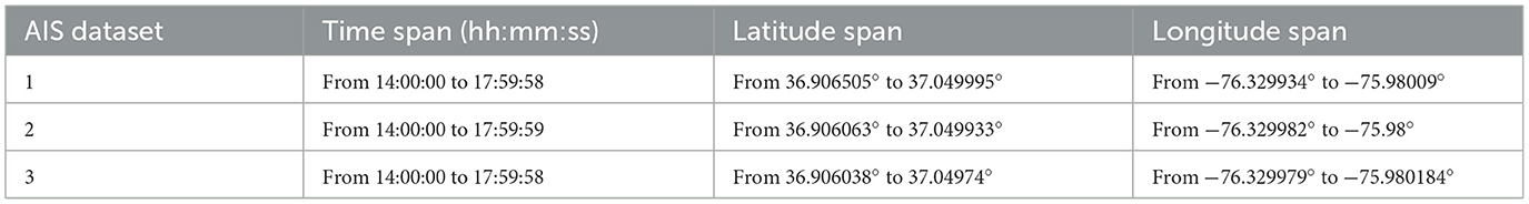
Table 1. The three AIS datasets.
We use the term trajectory reconstruction for estimating the AIS positions and connecting them as trajectories [6]. The existing works of trajectory reconstruction include linear interpolation, curvilinear interpolation [7], and its improvements [8, 9], and Recurrent Neural Networks (RNNs) [10]. Some of these methods employ physical models of movement information such as speeds, directions, and time, and typically use the speed over ground and course over ground, and others assume a distribution of vessel trajectories and train it from historical records [11, 12]. The state-of-the-art methods for trajectory reconstruction [13–15] generally have the following three steps: (1) apply a clustering method [16, 17] to group trajectories data according to their route patterns, (2) assign the vessel to one of these clusters, and (3) interpolate or predict the vessel trajectory based on the route pattern of the assigned cluster. However, these methods requires a training set of stationary patterns such as paths in long time and distances, and hence they are not applicable to the three AIS datasets that we analyzed consist of short-term and distances trajectories which lack the long-term patterns.
Our main contributions include: (1) The design of a novel big-data-compliant unsupervised algorithm which automatically learns and extracts useful spatiotemporal information from AIS data; (2) The proposed spatiotemporal features improve the accuracy of clustering the AIS points and reconstructing trajectories; (3) The proposed method has been successfully applied to reconstructed vessel trajectories with the real AIS data collected nearby Norfolk, Virginia, and simulated data. The highlights of this paper are summarized as follows. The proposed vessel trajectory reconstruction method utilizing the spatiotemporal characteristics of AIS data is unsupervised, and therefore it does not require a training set. The experimental results demonstrate the advantages of the proposed method when the training set is insufficient. Unlike the traditional clustering method, the proposed method uses the points with features represented by its projected positions based on speeds and angles, so the computation only involve local information and thus runs fast.
We first introduce the next-point concept with nearest neighbor classification method and then develop the nearest neighborhood clustering (NNC) when the vessel IDs are unknown using the proposed next-point method. We introduce a basic NNC method and design an advanced NNC trajectory reconstruction in this section. We will compare results of all these methods in the next section.
We convert the longitude and latitude into the Universal Transverse Mercator (UTM) coordinates, and then group the AIS points by the proposed nearest-neighbor clustering method. The next-point connection (NPC) clustering algorithm uses the distance defined as
where K is the index set of the AIS points in interval [t0, t] and dst is the space-time distance which is the Euclidean distance using all spatial and temporal features, [t0, t] is a preset search range of time (the interval length 1, 000 s used in our analysis), E and O stand for the estimated location and observed location at time t, respectively, and s is the set of variables used for finding the closest training points. The proposed clustering method contains the following steps:
• Step 1. Project each point's next location using its speed, direction, and the time differences between the point and its neighboring points.
• Step 2. Find the closest location for each estimated point's location Ei(s) from each label i ∈ K before the test point's time t0 ≤ s < t.
• Step 3. Assign the predicted label to the observed point O(t) based on its closest location Ei(s) in Step 2.
Although the NPC method is similar to the minimum spanning tree (MST) and single linkage cluster analysis (SLCA) [18, 19] that combine two clusters with the closest pair of points, NPC uses the estimated position E to measure the distance instead of the observed positions and NPC only searches AIS points in a nearby time interval. When the labels of the AIS points in K are known, the NPC method becomes a classification method and some points from the same vessel can be removed and only the AIS point with time closest to t will be used. The NPC methods that use the nearest neighbors to predict a vessel VID at each time t, they have the weaknesses: (1) NPC classification requires known labels which may not be available; (2) NPC clustering may merge different vessels and some feature with large values may dominate the distance. Therefore, we focus on the clustering method and propose the following algorithm to solve these issues.
We propose an clustering algorithm which is based on trajectory reconstruction and thus called CBTR, which builds the trajectories of vessels by using local physical information. CBTR is based on an NPC clustering method which uses doubly checked distance to improve accuracy. For each point is the data set, we select another point as its best possible next point (BPNP) and put them in the same cluster. Like MST and SLCA, BPNP groups all points into a dendrogram with several tree-type clusters because two distinct points might have the same BPNP. The trajectory can be visualized by connecting all points with its BPNP with a line segment. See Figure 6 for an illustration.
Given an AIS data set, in which points are ordered by their recording time ti, we denote each point by xi. The two-dimensional positions of xi on the earth are denoted as pi = [LAT(xi), LON(xi)] where LAT and LON stand for latitude and longitude of the AIS point x, and their speeds and courses are denoted by vi and ci, respectively. For every xi, we use its velocity, namely speed and course, to predict its future position and look for the best possible next point xj of it. If there is no point inside a reasonable searching range, then we consider xi as an endpoint of a trajectory. We trace each trail till an endpoint occurs and thus finish the clustering. So the algorithm of CBTR is designed as follows:
• Step 1. For a given point xi at time ti, we derive the linearly approximate future trajectory γi within 1,000 s by using its instant speed vi and course θ, i.e., the predicted position is defined by γi = xi + vi · ΔT, where ΔT is the time period which will be chosen in Step 2.
• Step 2. Collect all points appearing in the time zone t ∈ (ti, ti + 1000) and denote the collection as . Consider the closeness of γi and each point x in by computing a bi-directional distance D between γi and x, where ΔT is chosen to be the time difference between xi and x. Impose a spatiotemporal angle condition to exclude points with exaggerated turning course and denote the rest points as . Let the BPNP of xi be the one in the collection which has smallest D and satisfies the angle condition. Denote this smallest D as Di, namely, . When is empty, Di is defined to be infinity.
• Step 3. To choose a threshold in Step 3, we use the normalized distance . Sort all AIS points xi according to in descending order. Compute the ratio and find the first i whose ratio is less than a threshold (1.2 was used in our experiments). Take as a threshold and treat an AIS point as an endpoint of a projected line if its is larger than the threshold. At last, cluster vessels by using these endpoints.
The bi-directional distance D and the turning angle condition are the most crucial elements in CBTR, so we provide details of them as follows.
We compute the (squared) distance between γi and points in . If is small, then xj is probably the next AIS point of xi. However, as shown in Figure 1, there might be another vessel (colored in red) appearing in the direction of γi (the black arrow). In order to catch the correct BPNP xm for xi, we use the information of xm and xn to do double check. Precisely, we compute the backward locations σm and σn of xm and xn, respectively, namely the gray arrow and red arrow in Figure 1. One sees that the inconsistency between the black arrow and the red arrow can exclude xn as a BPNP of xi. On the other hand, xm is much possible to be the BPNP of xi because xi lies around the region that the gray arrow indicates. Therefore, we consider the bi-directional distance in Step 2. This (squared) bi-directional distance can resolve intersection problem in trajectory analysis.
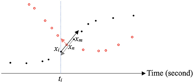
Figure 1. The direction of γi is indicated by the black arrow. The directions of σm and σn are indicated by the gray arrow and the red arrow, respectively. , the (squared) distance between xi and the end of gray arrow, is much smaller than . Hence xm is a better prediction than xn.
On the other hand, to prevent the endpoint of a trajectory connecting to another vessel, we have to impose a turning angle condition, which involves both space and time information. Roughly speaking, if the trajectory has to make a sudden unreasonable turn to connect its BPNP, then the trajectory should terminate right there. We cannot just measure the spatial angle because a vessel sometimes makes a large turn in a reasonable time period. So we need to consider a spatiotemporal angle. However, there is no natural exchange rate for temporal and spatial scales and we shall define a suitable one.
It is important to balance the scales of different spatiotemporal features for obtaining a meaningful space-time distance. The pooled normalization (a feature's values dividing by the range) and standardization (a feature's values divided by its standard error) are not suitable here, since the ranges of the spatiotemporal features of the vessels vary a lot. Consequently, we propose a dynamic scale conversion rate according to the vessel's speed and direction.
Considering that 1 knot is about 5·10−4 km/sec and the length of the diagonal of a longitude unit square is about 124.45 km in our data set, we choose τ = 4·10−6 ≈ 5·10−4/124.45 and α = 110.57/(111.32·cosθ), which are ratio estimators [20] to resale the data. The scaling factor α is used to convert unit of distance from degree of latitude into degree longitude so that they are comparable; the factor τ is used to normalize the time scale so that the temporal number looks in similar scale as spacial distance. Namely, for any two AIS points xi and xj, the spatiotemporal vector form xi to xj is defined by
where T(x) means the time of the AIS point x. When the angle φ between and γi is too large, say cos φ < 0.1, then we remove xj of candidates of BPNP of xi.
Definition 2.1 (Turning Angle Condition). The trajectory shall not make a sudden and unreasonable turn in which the spatiotemporal angle φ is greater than cos−1(0.1).
Thus we obtain from in Step 2. On the other hand, steady vessels with very slow movement which may be anchored float around with water currents and thus have randomly changing courses [21]. Therefore, for those steady pairs xi and xj with average speed smaller than 0.15 knots [22], we do not use the forward-backward distance and simply measure their D(xi, xj) by . The spatiotemporal vector representation in Equation (2) of the AIS points induces a linear model for the next point . Suppose that at the current time t0 the point is xi and at time s ∈ (t0, t) the point is , and , we use the current speed speed(xi) and angel θ(xi) to approximate the dynamic speed and angle from time t0 to time s so that the moving distance that has the true value from an integral of the dynamic speed over time (t0, s) is estimated by the product of moving time and speed, and y2 and y3 come from the first-order Taylor polynomial of the angle around xi that is used for cosine and sine. Consequently, we have the following regression models
where , , , and and are white noises that can be viewed as the errors from the linear approximations of the speed and angle.
In pursuit of better performance, we consider different values of parameter τ according to the types of vessels. However, the types of vessels are not provided in our AIS data. Alternatively, we adjust the value of τ based on the speed of vessels. This method is essentially a ratio estimator in cluster sampling [23]. For faster vessels with speed larger than 4 knots, we use larger τ, 4·10−5, so that the time difference is scaled to be comparable to the spatial difference in . For slower vessels with speed smaller than four knots, we use τ = 4·10−5 as proposed in the above paragraph. To demonstrate the performance of CBTR on different types of vessels, we present individual results of four categories of vessels according to their speeds: (1) xi and xj are called a high speed pair if the average speed (in knots) S of them is larger than or equal to 16 knots; (2) fast pair if 4 ≤ S < 16; (3) slow pair if 0.15 ≤ S < 4; (4) steady pair if S < 0.15. We use τ = 4·10−5 for vessels of the fist two categories, which have faster speeds, and use τ = 4·10−6 for vessels of the last two categories. The results are shown in Table 5.
The proposed CBTR algorithm can be viewed as a special case of the weighted-average plug-in classifier [24, 25], with weights given by wi(x) = 1/k if xi is one of the k nearest neighbors of x in the search range S, and wi(x) = 0 otherwise. Stone's theorem establishes consistency of the proposed clustering method provided that the weights satisfy certain conditions [26].
We evaluated the results by the correct-neighbor rate that is defined as where Yj is the label of the closest neighbor of Yi. In the CBTR algorithm, every AIS point is either assigned a BPNP or determined as an endpoint of a trajectory. We sum up all mistakes made in this process, say M, and compute the correct-neighbor rate as 1−M/n. The proposed method does not aim to find a correct sequential pattern of a trajectory. The definition of the accuracy used in this article only considers the correct clustered labels in the beginning of Section 3.1. It means that it is possible that the proposed method groups one vessel's AIS points in the order of (1, 3, 2) although the true order is (1, 2, 3). However, in this case, it is considered as a correct clustering result.
We compare the CBTR with other methods including the LSTM recurrent neural network (RNN) architecture [27–29] and the EM clustering algorithm [30, 31] which assumes mixed Gaussian distributed clusters. The Expectation-Maximization (EM) algorithm using a Gaussian mixture model estimates the probability of each observation iteratively through the E-step and M-step. Each EM cluster is determined by its mean and variance, so that it is suitable for vessels that are anchored or moving randomly in a fixed location. Since most vessels are moving with varying speeds and directions, the EM clustering does not perform well in the datasets. The comparisons of their correct-neighbor rates are listed in Tables 2, 3.
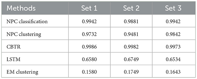
Table 2. The correct-neighbor rates for each method of the AIS data with speed >3 knots in the three datasets.
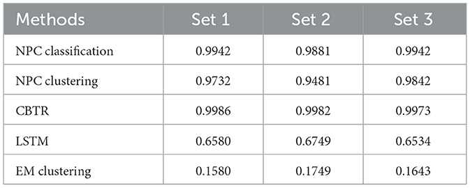
Table 3. The correct-neighbor rates for each method of the AIS data with speed ≤ 3 knots in the three datasets.
The time complexity of the proposed CBTR method is O(nr) with the sample size n and the neighborhood size r. See the computational time for each method in Table 4.
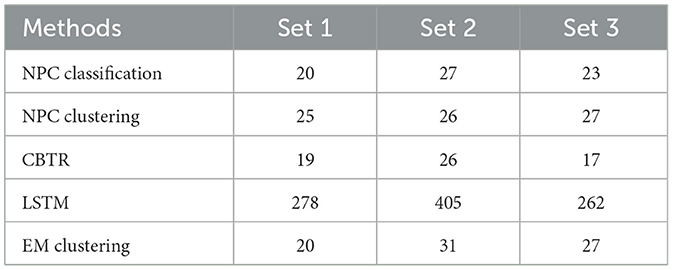
Table 4. The computational time for each method in the three datasets in seconds.
In Figures 2, 3, one sees that CBTR is able to regroup most of the trajectories correctly. We leave the detailed explanation of these plots in the Supplementary material. One may evaluate the performance of CBTR by two numbers: jumps and merges. The former counts the total breaks of trajectories done wrongly by CBTR and the later counts how many wrong groupings CBTR makes. Instead of counting how many points are connected to wrong next point, the sum of jumps and merges shows the performance of CBTR more faithfully. Since each jump creates a new clustering and each merge cancels a group, the difference between them is exactly the difference between the number of vessels of our data and the number of clusters via CBTR. Namely we have the following identity: merges − jumps = #{predicted clusters}−#{actual number of vessels}.
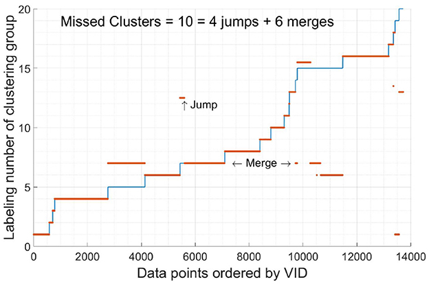
Figure 2. The clustering results of data set 1. The numbers in the horizontal axis are ordered by the vessels' VIDs. The red lines are the predicted labels and the blue lines are the true labels. Most points of vessel no. 7 are merged with vessel no. 5 and the rest points are split into another cluster independent from other vessels. Vessel no. 15 is merged with vessel no. 5 and no. 6, and contributes 2 jumps.
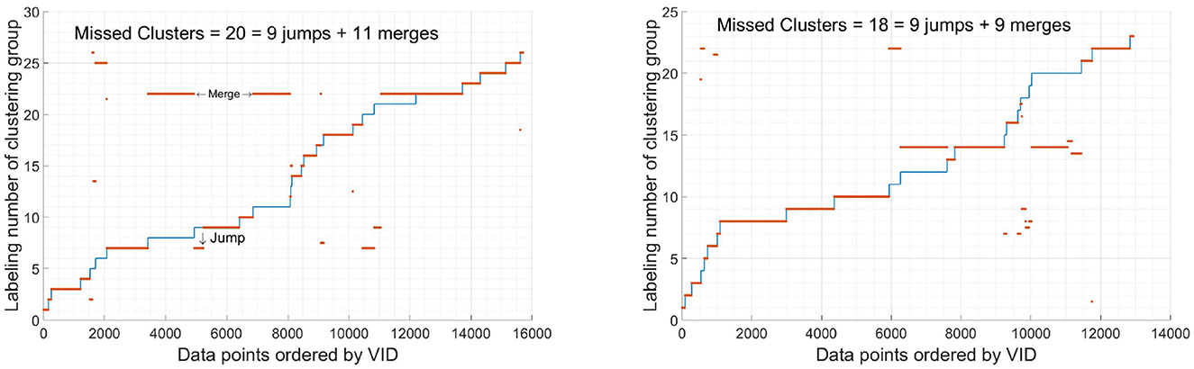
Figure 3. The clustering results of data set 2 and data set 3.
In order to evaluate the robustness of CBTR, we conducted experiments by removing points in the data sets so that the trajectories become harder to be tracked. Indeed, we consider validation sets by method 1: removing each fifth point of every five points (i.e., the fifth, tenth, etc.) and method 2 removing each second point of every two points (i.e., the second, fourth, etc.). In sum, we take out 20 and 50% points, respectively, in each validation set and apply CBTR to predict the trajectories. For the downsampled AIS datasets 1, 2, 3 using method 1, the correct rates of the estimated neighbors are 0.9977, 0.9977, and 0.9966, respectively. For the downsampled AIS datasets 1, 2, 3 using method 2, the correct rates of estimated neighbors are 0.9947, 0.9943, and 0.9913, respectively. As we anticipated, the more points are removed, the lower the correct rates of estimated neighbors are. However, CBTR still performs very well whereas large amounts of points are removed. Furthermore, we remark that there is a trade-off between the reduction of the number of jumps and the increment of the number of mergers. If the upper bound for time interval is lager than 1,000 in Step 1, it may lead to more candidates used for selecting BPNP and fewer jumping points while increases the number of merges.
The predicted trajectories of all vessels in data set 1 by using CBTR are shown in Figure 4. From the left-hand boundary of this picture, we know the data set contains some incomplete trajectories and it is impossible to cluster them correctly. One can see a zoomed-in picture of this boundary phenomenon in Figure 5.
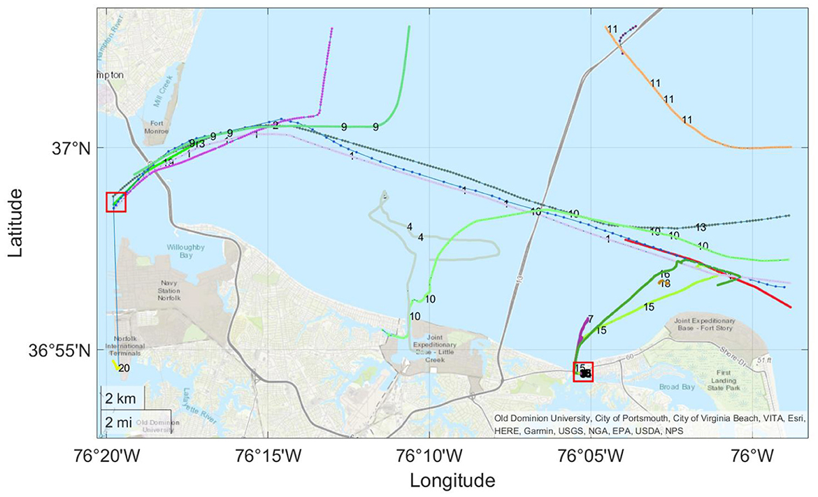
Figure 4. The predicted trajectories of all vessels in data set 1 by using CBTR. Points are colored and lined according to clusters and are numbered by the actual VIDs. Two red boxed regions will be enlarged in the following figures. Most of the trajectories are clustered correctly. The only visible errors in this picture are the merge of vessels no. 1 and no. 19 and the merge of vessels no. 13 and no. 20 (in the middle left). Details in the two red boxes are shown as Figures 5, 6.
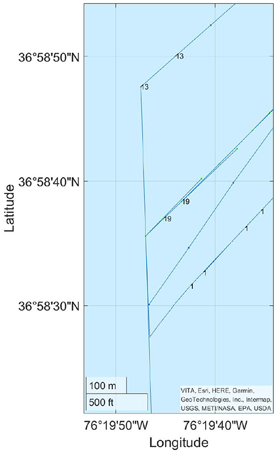
Figure 5. Points are colored and lined according to clusters and are numbered by the actual VIDs. The merge of vessel no. 19 to vessel no. 1 is due to the limit of boundary of the dataset. Vessel no. 13 is connected to no. 20, which is outside the plot, due to the same boundary effect.
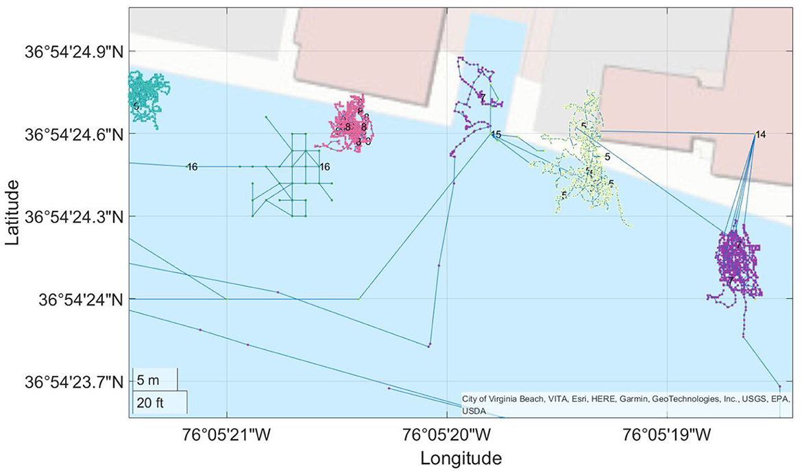
Figure 6. The predicted trajectories of vessel no. 5–8 and no. 14–16. Points are colored and lined according to clusters and are numbered by the actual VIDs. Points of vessel no. 14 are merged to others due to their problematic location. On the other hand, the endpoint of vessel no. 5 is incorrectly connected to a point of vessel no. 7. Vessel no. 8, which is steady, is perfectly clustered.
Figure 6 shows another mistake made by CBTR. This kind of mistakes happens at the endpoint of some trajectories. To be precise, when a vessel goes back and parks at a pier, it will turn off the AIS signal transmitter. The last position reported shall be the endpoint of the trajectory. But sometimes CBTR finds a false next point for this endpoint and continues the trial. For example, in Figure 6, vessel no. 7 (colored purple) left toward west, came back, and parked to the east of vessel no. 5. At that moment, vessel no. 5 was reporting its last location before turning off its signal transmitter. CBTR found some point of vessel no. 7 to be a possible next point of the last point of vessel no. 5. So it makes a wrong connection from the circled point to the squared point. This is called a terminal-type mistake and counted as a merge.
These terminal-type mistakes only happen when two vessels are anchored close to each other. We can prevent this terminal-type mistakes by using more restrictive connecting criterion, but this will break some trajectories of moving vessels because AIS points in moving trajectories are much sparser than AIS points in steady vessels moored to the piers. In this case, the speed and angle of a vessel randomly change by wave drift forces, so the variances of the white noises in our model (3) may be larger than the signals (speed). These terminal-type mistakes are not that serious because the AIS data is mainly used to recognize moving vessels. Except the boundary phenomenon and the terminal-type mistakes, CBTR performs perfectly on generic situations and is a reliable method to predict trajectories. Table 5 shows the performance of CBTR for vessels with different speeds. One can see that slow vessels are the most challenging ones for CBTR.
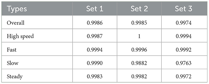
Table 5. Performance of vessels of different types.
Long Short-Term Memory [27] is a type of Recurrent Neural Networks (RNNs). LSTMs are an example of a recurrent neural network which has feedback loops allowing time-dependent problems to be solved. That is, the outputs (i.e., previous outputs) can be used as an input to help model the current output. More generally, problems that have a fundamental order can be solved. LSTMs are capable of modeling sequences of different lengths, and this is ideal as vessel paths often have a different number of points [32].
LSTMs have been used for predicting vessel trajectories with AIS data [33–35] as they can naturally be adapted to multi-target learning and are capable of learning both simple and complex patterns. Here we can think of the timestamp, latitude, longitude, speed, and direction, all at time t, as response variables whereas the predictor variables (i.e., inputs to the LSTM) are the timestamp, latitude, longitude, speed, and direction at time t−1, t−2, ⋯ , t−k. We train an LSTM using lagged versions of the timestamp, latitude, longitude, speed, and direction (i.e., time t−1, t−2.⋯ , t−k) in order to predict the timestamp, latitude, longitude, speed, and direction at one time point in the future (i.e., time t). The goal here is to attempt to predict all characteristics of a vessel automatically using previous information. The architecture and tuning were accomplished via trial an error using a random 20% validation sample.
The characteristics of the LSTM are the following: an input dimension of 5 (i.e., timestamp, latitude, longitude, speed, and direction are lagged by k = 1 time unit), 1 hidden layer, 250 hidden units using the Rectified Linear Unit (ReLU) activation function: max(0, x), and 5 output nodes (i.e., timestamp, latitude, longitude, speed, and direction at time t). Additional values for the number of lags were tried, but the performance was essentially unchanged and different activation functions were tried and tended to produce inferior results. The software used was the keras library in Python [36].
The results from the LSTM using all five variables as outputs seem to indicate that this approach is unable to distinguish the different vessel trajectories due to several reasons including the initial value and the training set of LSTM [33], the changes of courses and speeds [34] in the given prediction time range, and the normalization method [35] which may over-compress trajectory data since the some trajectories have large ranges but others do not.
The performance of the LSTM next point prediction method is fundamentally dependent on the historical trajectories with labels used to train the LSTM model to predict the properties of the node at the next time point [32, 37]. That is, the training set with labeled trajectories are needed to accurately predict the timestamp, latitude, longitude, speed, and direction at some future point in time. However, to make a fair comparison, only the current AIS point is used in training a LSTM model for predicting the next point, and this makes the recurrent neurons not able to sufficiently learn the latent features in the AIS datasets and leads to inaccurate prediction [38, 39]. LSTM models are known to require a large amount of data in order to be effective, so the relatively small size of the individual AIS training datasets also is a contributing factor to the LSTM's performance.
An inspection of the LSTM predictions and the resulting nearest neighbor search indicate that most of the errors are related primarily to two factors: some vessels rapidly change their speed and direction while simultaneously other vessels that were previously similar to the rapidly changing vessel do not change their speed or direction suddenly and this results in misclassification, for example, vessels no. 5–8. The second source of error may be that the predicted AIS points by LSTM have large variations [37] and in combination with a larger number of candidates within each time window (i.e., the time window in the nearest neighbor search), mistakes are accumulated.
The proposed CBTR method successfully cluster AIS points and track a trajectory without knowing the true labels of AIS points. Step 2 of the proposed CBTR is the essence of our method, which integrates the forward and backward estimated positions into measuring the differences between two adjacent points. This step evaluates how good the fitted path is dynamically instead of using the static point information by measuring the mutual distances between points. Thus, CBTR algorithm is able to distinguish intersecting trajectories. The second feature in Step 2 is to define a suitable parameter τ to exchange time and space scales. Therefore, CBTR is applicable to various kinds of moving-point data lacking in labels, and its spatiotemporal features can be used with other methods [40] to select a safe maneuver crossing scenario with two target ships.
The datasets presented in this study can be found in online repositories. The names of the repository/repositories and accession number(s) can be found at: https://gitlab.com/algorithms-for-threat-detection/2019/atd2019.
H-HH and C-WC reviewed literature and designed the proposed methods. C-WC wrote and ran the Matlab code for the proposed CBTR method and edited the proposed methodology and the analysis results. H-HH drafted the manuscript. All authors proofread the manuscript. All authors contributed to the article and approved the submitted version.
This research was supported in part by the National Science Foundation grant, DMS-1924792 and MOST Young Scholar Fellowship Program, grant no. NSTC 112-2636-M-110-007.
C-WC thanks the support from National Center for Theoretical Sciences in Taiwan.
The authors declare that the research was conducted in the absence of any commercial or financial relationships that could be construed as a potential conflict of interest.
All claims expressed in this article are solely those of the authors and do not necessarily represent those of their affiliated organizations, or those of the publisher, the editors and the reviewers. Any product that may be evaluated in this article, or claim that may be made by its manufacturer, is not guaranteed or endorsed by the publisher.
The Supplementary Material for this article can be found online at: https://www.frontiersin.org/articles/10.3389/fams.2023.1124091/full#supplementary-material
1. Mankabady S. The International Maritime Organization, Volume 1: International Shipping Rules. Cambridge: Cambridge University Press (1986).
2. Natale F, Gibin M, Alessandrini A, Vespe M, Paulrud A. Mapping fishing effort through AIS data. PLoS ONE. (2015) 10:e0130746. doi: 10.1371/journal.pone.0130746
3. Mercer D,. Algorithms for Threat Detection 2019 Challenge AIS Data. (2019). Available online at: https://gitlab.com/algorithms-for-threat-detection/2019/atd2019 (accessed October 28, 2020).
4. Bautista-Sánchez R, Barbosa-Santillan LI, Sánchez-Escobar JJ. Method for select best AIS data in prediction vessel movements and route estimation. Appl Sci. (2021) 11:2429. doi: 10.3390/app11052429
5. Mehrholz D, Leushacke L, Flury W, Jehn R, Klinkrad H, Landgraf M. Detecting, tracking and imaging space debris. ESA Bull. (2002) 128–34.
6. Young BL. Predicting Vessel Trajectories From AIS Data Using R. Monterey, CA: Naval Postgraduate School Monterey (2017).
7. Best RA, Norton JP. A new model and efficient tracker for a target with curvilinear motion. IEEE Trans Aerospace Electron Syst. (1997) 33:1030–7. doi: 10.1109/TAES.1997.599329
8. Perera LP, Oliveira P, Soares CG. Maritime traffic monitoring based on vessel detection, tracking, state estimation, and trajectory prediction. IEEE Trans Intell Transp Syst. (2012) 13:1188–200. doi: 10.1109/TITS.2012.2187282
9. Schubert R, Richter E, Wanielik G. Comparison and evaluation of advanced motion models for vehicle tracking. In: 2008 11th International Conference on Information Fusion. Cologne (2008). p. 1–6.
10. Nguyen D, Vadaine R, Hajduch G, Garello R, Fablet R. A multi-task deep learning architecture for maritime surveillance using AIS data streams. In: 2018 IEEE 5th International Conference on Data Science and Advanced Analytics (DSAA). Turin (2018). p. 331–40. doi: 10.1109/DSAA.2018.00044
11. Millefiori LM, Braca P, Bryan K, Willett PK. Modeling vessel kinematics using a stochastic mean-reverting process for long-term prediction. IEEE Trans Aerospace Electron Syst. (2016) 52:2313–30. doi: 10.1109/TAES.2016.150596
12. Pallotta G, Horn S, Braca P, Bryan KB. Context-enhanced vessel prediction based on ornstein-uhlenbeck processes using historical AIS traffic patterns: real-world experimental results. In: 17th International Conference on Information Fusion. Vol. 4. Salamanca (2014). p. 213.
13. Mazzarella F, Arguedas VF, Vespe M. Knowledge-based vessel position prediction using historical AIS data. In: 2015 Sensor Data Fusion: Trends, Solutions, Applications (SDF). Bonn (2015). p. 1–6. doi: 10.1109/SDF.2015.7347707
14. Hexeberg S, Flaten AL, Eriksen BOH, Brekke EF. AIS-based vessel trajectory prediction. In: 2017 20th International Conference on Information Fusion (Fusion). Xi'an (2017). p. 1–8. doi: 10.23919/ICIF.2017.8009762
15. Coscia P, Braca P, Millefiori LM, Palmieri FAN, Willett PK. multiple Ornstein-Uhlenbeck processes for maritime traffic graph representation. IEEE Trans Aerospace Electron Syst. (2018) 54:2158–70. doi: 10.1109/TAES.2018.2808098
16. Lee JG, Han J, Whang KY. Trajectory clustering: a partition-and-group framework. In: Proceedings of the 2007 ACM SIGMOD International Conference on Management of Data. SIGMOD'07. New York, NY: ACM (2007). p. 593–604. doi: 10.1145/1247480.1247546
17. Pallotta G, Vespe M, Bryan K. Vessel pattern knowledge discovery from AIS data: a framework for anomaly detection and route prediction. Entropy. (2013) 15:2218–45. doi: 10.3390/e15062218
18. Gower JC, Ross GJ. Minimum spanning trees and single linkage cluster analysis. J R Stat Soc Ser C. (1969) 18:54–64. doi: 10.2307/2346439
19. Huang HH, Yu C, Zheng H, Hernandez T, Yau SC, He RL, et al. Global comparison of multiple-segmented viruses in 12-dimensional genome space. Mol Phylogenet Evol. (2014) 81:29–36. doi: 10.1016/j.ympev.2014.08.003
20. Scott A, Wu CF. On the asymptotic distribution of ratio and regression estimators. J Am Stat Assoc. (1981) 76:98–102. doi: 10.1080/01621459.1981.10477612
21. Silber GK, Adams JD, Fonnesbeck CJ. Compliance with vessel speed restrictions to protect North Atlantic right whales. PeerJ. (2014) 2:e399. doi: 10.7717/peerj.399
22. Redoutey M, Scotti E, Jensen C, Ray C, Claramunt C. Efficient vessel tracking with accuracy guarantees. In: International Symposium on Web and Wireless Geographical Information Systems. London: Springer (2008). p. 140–51. doi: 10.1007/978-3-540-89903-7_13
23. Dryver AL, Chao CT. Ratio estimators in adaptive cluster sampling. Environmetrics. (2007) 18:607–20. doi: 10.1002/env.838
24. Wang J, Shen X, Liu Y. Probability estimation for large-margin classifiers. Biometrika. (2008) 95:149–67. doi: 10.1093/biomet/asm077
25. Wu Y, Zhang HH, Liu Y. Robust model-free multiclass probability estimation. J Am Stat Assoc. (2010) 105:424–36. doi: 10.1198/jasa.2010.tm09107
26. Stone CJ. Consistent nonparametric regression. Ann Stat. (1977) 5:595–620. doi: 10.1214/aos/1176343886
27. Hochreiter S, Schmidhuber J. Long short-term memory. Neural Comput. (1997) 9:1735–80. doi: 10.1162/neco.1997.9.8.1735
28. Ding M, Su W, Liu Y, Zhang J, Li J, Wu J. A novel approach on vessel trajectory prediction based on variational LSTM. In: 2020 IEEE International Conference on Artificial Intelligence and Computer Applications (ICAICA). Dalian (2020). p. 206–11. doi: 10.1109/ICAICA50127.2020.9182537
29. Jin J, Zhou W, Jiang B. Maritime target trajectory prediction model based on the RNN network. In: Artificial Intelligence in China. Berlin: Springer (2020). p. 334–42. doi: 10.1007/978-981-15-0187-6_39
30. Dempster AP, Laird NM, Rubin DB. Maximum likelihood from incomplete data via the EM algorithm. J R Stat Soc Ser B. (1977) 39:1–22. doi: 10.1111/j.2517-6161.1977.tb01600.x
31. Rubin DB, Thayer DT. EM algorithms for ML factor analysis. Psychometrika. (1982) 47:69–76. doi: 10.1007/BF02293851
32. Capobianco S, Millefiori LM, Forti N, Braca P, Willett P. Deep learning methods for vessel trajectory prediction based on recurrent neural networks. IEEE Trans Aerospace Electron Syst. (2021) 57:4329–46. doi: 10.1109/TAES.2021.3096873
33. Tang H, Yin Y, Shen H. A model for vessel trajectory prediction based on long short-term memory neural network. J Mar Eng Technol. (2019) 21:136–45. doi: 10.1080/20464177.2019.1665258
34. Forti N, Millefiori LM, Braca P, Willett P. Prediction of vessel trajectories from AIS data via sequence-to-sequence recurrent neural networks. In: ICASSP 2020-2020 IEEE International Conference on Acoustics, Speech and Signal Processing (ICASSP). Barcelona (2020). p. 8936–40. doi: 10.1109/ICASSP40776.2020.9054421
35. Zhang Z, Ni G, Xu Y. Ship trajectory prediction based on LSTM neural network. In: 2020 IEEE 5th Information Technology and Mechatronics Engineering Conference (ITOEC). Chongqing (2020). p. 1356–64. doi: 10.1109/ITOEC49072.2020.9141702
36. Chollet F,. Deep Learning with Python. Simon Schuster (2021). Available online at: https://github.com/keras-team/keras
37. Gao DW, Zhu YS, Zhang JF, He YK, Yan K, Yan BR. A novel MP-LSTM method for ship trajectory prediction based on AIS data. Ocean Eng. (2021) 228:108956. doi: 10.1016/j.oceaneng.2021.108956
38. Sagheer A, Kotb M. Unsupervised pre-training of a deep LSTM-based stacked autoencoder for multivariate time series forecasting problems. Sci Rep. (2019) 9:1–16. doi: 10.1038/s41598-019-55320-6
39. Suo Y, Chen W, Claramunt C, Yang S. A ship trajectory prediction framework based on a recurrent neural network. Sensors. (2020) 20:5133. doi: 10.3390/s20185133
Keywords: Automatic Identification System (AIS), clustering, Long Short-Term Memory (LSTM), trajectory prediction, trajectory reconstruction
Citation: Chen C-W and Huang H-H (2023) Unsupervised vessel trajectory reconstruction. Front. Appl. Math. Stat. 9:1124091. doi: 10.3389/fams.2023.1124091
Received: 14 December 2022; Accepted: 27 February 2023;
Published: 17 March 2023.
Edited by:
Eric Chung, The Chinese University of Hong Kong, ChinaReviewed by:
Stefano Marrone, Università Della Campania “Luigi Vanvitelli”, ItalyCopyright © 2023 Chen and Huang. This is an open-access article distributed under the terms of the Creative Commons Attribution License (CC BY). The use, distribution or reproduction in other forums is permitted, provided the original author(s) and the copyright owner(s) are credited and that the original publication in this journal is cited, in accordance with accepted academic practice. No use, distribution or reproduction is permitted which does not comply with these terms.
*Correspondence: Hsin-Hsiung Huang, aHNpbi1oc2l1bmcuaHVhbmdAdWNmLmVkdQ==
Disclaimer: All claims expressed in this article are solely those of the authors and do not necessarily represent those of their affiliated organizations, or those of the publisher, the editors and the reviewers. Any product that may be evaluated in this article or claim that may be made by its manufacturer is not guaranteed or endorsed by the publisher.
Research integrity at Frontiers
Learn more about the work of our research integrity team to safeguard the quality of each article we publish.