GPMatch: A Bayesian causal inference approach using Gaussian process covariance function as a matching tool

A Gaussian process (GP) covariance function is proposed as a matching tool for causal inference within a full Bayesian framework under relatively weaker causal assumptions. We demonstrate that matching can be accomplished by utilizing GP prior covariance function to define matching distance. The matching properties of GPMatch is presented analytically under the setting of categorical covariates. Under the conditions of either (1) GP mean function is correctly specified; or (2) the GP covariance function is correctly specified, we suggest GPMatch possesses doubly robust properties asymptotically. Simulation studies were carried out without assuming any a priori knowledge of the functional forms of neither the outcome nor the treatment assignment. The results demonstrate that GPMatch enjoys well-calibrated frequentist properties and outperforms many widely used methods including Bayesian Additive Regression Trees. The case study compares the effectiveness of early aggressive use of biological medication in treating children with newly diagnosed Juvenile Idiopathic Arthritis, using data extracted from electronic medical records. Discussions and future directions are presented.

1. Introduction

Data from nonrandomized experiments, such as registries and electronic records, are becoming indispensable sources for answering causal inference questions in health, social, political, economics, and many other disciplines. Under the assumptions of no unmeasured confounders, ignorable treatment assignment, and distinct model parameters governing the science and treatment assignment mechanisms, Rubin [1] suggested Bayesian approach to the estimation of causal treatment effect can be accomplished by directly modeling the outcomes, treating it as a missing potential outcome problem. Direct modeling is able to utilize the many Bayesian regression modeling techniques to address complex data types and data structures, such as examples in Hirano et al. [2], Zajonc [3], Imbens and Rubin [4], and Baccini et al. [5]. Recent work further suggested that outcome regression-based estimation should be asymptotically more efficient than any inverse probability weighting-based estimation [6].

Parameter-rich Bayesian modeling techniques are particularly appealing as they do not presume a known functional form, and thus may help mitigate potential model misspecification issues. Hill [7] suggested Bayesian additive regression tree (BART) can be used for causal inference, and showed it produced more accurate estimates of average treatment effects compared to propensity score matching, inverse propensity weighted estimators, and regression adjustment in the nonlinear setting, and it performed as well under the linear setting. Others have used Gaussian Process in conjunction with Dirichlet Process priors, e.g., Roy et al. [8] and Xu et al. [9]. Roy et al. [10] devised enriched Dirichlet Process priors tackling missing covariate issues. However, naive use of regression techniques could lead to substantial bias in estimating causal effect as demonstrated in Hahn et al. [11].

The search for ways of incorporating propensity of treatment selection into the Bayesian causal inference has been long-standing. Including propensity score (PS) as a covariate in the outcome model may be a natural way. However, joint modeling of outcome and treatment selection models leads to a “feedback” issue. A two-staged approach was suggested by McCandless et al. [12], Zigler et al. [13], and others. Whether the uncertainty of the first step propensity score modeling should be taken into account when obtaining the final result in the second step remain a point of discussion [14–17]. Saarela et al. [18] proposed an approximate Bayesian approach incorporating inverse probability treatment assignment probabilities as importance-sampling weights in Monte Carlo integration. It offers a Bayesian version of the augmented inverse probability treatment weighting (AIPTW). Hahn et al. [19] suggested incorporating estimated treatment propensity into the regression to explicitly induce covariate dependent prior in the regression model. These methods all require a separate step of treatment propensity modeling, which may suffer if the propensity model is misspecified.

Matching is one of the most sought-after methods used for the design and analyzes of observational studies for answering causal questions. Matching experimental units on their pre-treatment assignment characteristics helps to remove the bias by ensuring the similarity or balance between the experimental units of the two treatment groups. Matching methods impute the missing potential outcome with the value from the nearest match or the weighted average of the values within the nearby neighborhood defined by (a chosen value) caliper. Matching on multiple covariates could be challenging when the dimensions of the covariates are large. For this reason, matching is often performed using the estimated propensity score (PS) or by the Mahalanobis distance (MD). The idea is, under the no unmeasured confounder setting, matching induces a balance between the treated and untreated groups. Therefore, it serves to transform a nonrandomized study into a pseudo-randomized study. There are many different matching techniques, a comprehensive review is provided in Stuart [20]. A recent study by King and Nielsen [21] compared PS matching with MD matching and suggests that PS matching can result in a more biased and less accurate estimate of averaged causal treatment as the precision of matching improves, while MD matching is showing improved accuracy. Common to matching methods, the data points without a match are discarded. Such a practice may lead to a sample no longer representative of the target population. A user-specified caliper is often required, but different calipers could lead to very different results. Furthermore, matching on a miss-specified PS could lead to invalid causal inference results.

A combination of matching and regression is a better approach than using either of them alone [22]. Ho et al. [15] advocated matching as nonparametric preprocessing for reducing dependence on parametric modeling assumptions. Gutman and Rubin [23] examined different strategies of combining the preprocessed matching with a regression modeling of the outcome through extensive simulation studies. They demonstrated that some commonly used causal inference methods have poor operating characteristics, and consider ways to correct for variance estimate for causal treatment effect obtained from regression modeling after preprocessed matching. To our knowledge, no existing method can accomplish matching and regression modeling in a single step.

Gaussian process (GP) prior has been widely used to describe biological, social, financial, and physical phenomena, due to its ability to model highly complex dynamic systems and its many desirable mathematical properties. Recent literature, e.g., Choi and Woo [24] and Choi and Schervish [25], has established posterior consistency for Bayesian partially linear GP regression models. Bayesian modeling with GP prior can be viewed as a marginal structural model where the treatment effect is modeled as a linear function of background variables. It predicts the missing response by a weighted sum of observed data, with larger weights assigned to those in closer proximity but smaller to those further away, much like a matching procedure. This motivated us to consider using GP prior covariance function as a matching tool for Bayesian causal inference.

The idea of utilizing GP prior in a Bayesian approach to causal inference is not new. Examples can be found in Roy et al. [8] for addressing heterogeneous treatment effect, in Xu et al. [9] for handling dynamic treatment assignment, and in Roy et al. [10] for tackling missing data. While these studies demonstrated GP prior could be used to achieve flexible modeling and tackle complex settings, no one has considered GP prior a matching tool. This study adds to the literature in several ways. First, we offer a principled approach to Bayesian causal inference utilizing GP prior covariance function as a matching tool, which accomplishes matching and flexible outcome modeling in a single step. Second, we provide relaxed causal assumptions than the widely adopted assumptions from the landmark paper by Rosenbaum and Rubin [26]. By admitting additional random noise in outcome measures, these new assumptions fit more naturally within the Bayesian framework. Under these weaker causal assumptions, the GPMatch method offers a doubly robust approach in the sense that the averaged causal treatment effect is correctly estimated when either one of the conditions is met: (1) when the mean function correctly specifies the prognostic function of outcome; or (2) the covariance function matrix correctly specifies the treatment propensity.

The rest of the presentation is organized as follows. Section 2 describes methods, where we present problem setup, causal assumptions, and the model specifications. The utility of the GP covariance function as a matching tool is presented in Section 3, followed by discussions of its double robustness property. Simulation studies are presented in Section 4. Simulations are designed to represent the real-world setting where the true functional form is unknown, including the well-known simulation design suggested by Kang and Schafer [27]. We compared the GPMatch approach with some commonly used causal inference methods, i.e., linear regression with PS adjustment, inverse probability treatment weighting, and BART, without assuming any knowledge of the true data-generating models. The results demonstrate that the GPMatch enjoys well-calibrated frequentist properties, and outperforms many widely used methods under the dual misspecification setting. Section 5 presents a case study, examining the comparative effectiveness of an early introduction of biological medication in treating children with recently diagnosed juvenile idiopathic arthritis (JIA). Section 6 presents the summary, discussions, and future directions.

2. Method

2.1. Notations, problem setup, and parameters of interests

For the i^th sample unit, we observe D_i = (X_i, A_i, Y_i), i =, 1..., n, a random sample of a given study population. Denote the causal factor or “treatment” by A_i. For simplicity of exposition, here we consider A_i = 1/0. Let Y_i denote the observed outcomes, X_i the p-dimensional observed vector of background variable, which contains determinants of treatment assignment Pr(A_i = 1) = π(x_i) and the determinants of potential outcomes $Y_i^{(a)}=f^{(a)}(x_i),a\in {A}$. Given the background variables X_i, such as patient age, gender, genetic makeup, disease status, environmental exposures, and past treatment histories, the potential outcomes for a given patient are determined by the underlying science mechanisms $f^{(a)}({\mathit{x}}_i)$, and the treatment are assigned following A_i~Ber(π(x_i)).

Under the given treatment assignment, the observed outcome may be measured with error, i.e., a noisy version of the corresponding potential outcomes,

$\begin{array}{ll}{Y}_i=Y_i^{(0)}(1-A_i)+Y_i^{(1)}{A}_i+{ϵ}_i,& (1)\end{array}$

where E(ϵ_i) = 0. In other words, the observed outcome for the i^th individual is a realization of the joint actions between the science mechanisms and the treatment assignment. Any two sample units that share the same background features X_i = X_j = x, regardless of their treatment assignment, are expected to experience the same potential outcomes $E(Y_i|x)=E(Y_j|x)=f^{(a)}(x)$.

Our goal is to estimate the averaged treatment effect for a given study population

$\begin{array}{ll}ATE=E(\tau (x)),& (2)\end{array}$

where τ(x) = f⁽¹⁾(x)−f⁽⁰⁾(x).

2.2. The causal assumptions

To ensure identifiability of the causal treatment effect, we impose the following causal assumptions, which may be considered as a somewhat relaxed version of commonly adopted causal assumptions as suggested in Rosenbaum and Rubin [26]:

CA1. Stable Unit Treatment Value Expectation Assumption (SUTVEA).

(i) We consider the observed outcome may be a noisy version of the potential outcome where the expectation of the observed outcome is jointly determined by the underlying science mechanisms and the treatment assignment $E(Y_i)=f_i^{(0)}(1-A_i)+f_i^{(1)}{A}_i$, for A_i = 0, 1.

(ii) For the underlying science mechanism that generates potential outcomes, there exists a constant K > 0 such that |f^(a)| ≤ K, for a = 0, 1.

CA2. Ignorable Treatment Assignment Assumption, or no unmeasured confounders assumption requires the treatment assignment is independent from the underlying science mechanism given the observed covariates, $A_i\perp f^{(a)}|X_i$ for a = 0, 1 .

CA3. Positivity Assumption. For every sample unit, there is a nonzero probability of being assigned to either one of the treatment arms, i.e., 0 < Pr(A_i|X_i) < 1.

The SUTVEA assumption represents a somewhat weaker assumption than SUTVA. It acknowledges the existence of residual random error in the outcome measure. The observed outcomes may differ from the corresponding true potential outcomes due to some measurement errors or account for random noise related to the treatment received. For example, outcomes could differ by recorders, the timing of the treatment, the pre-surgery preparation procedure, or the concomitant medication. In addition, we consider the potential outcomes from different experimental units may be correlated, where the correlations are determined by the covariates. Under the no unmeasured confounders assumption, we may model the correlation between two potential outcomes. Since only one of all potential outcomes could be observed, the causal inference presents a highly structured missing data setup where the correlations between $(Y_i^{(1)},Y_i^{(0)})$ are not directly identifiable. Admitting residual random errors and allowing for explicit modeling of the covariance structure, the new assumptions may facilitate better statistics inference.

2.3. Model specifications

The marginal structural model (MSM) is a widely adopted modeling approach to causal inference, which serves as a natural framework for Bayesian causal inference. The MSM specifies

$\begin{array}{l}{Y}_i^{(1)}=Y_i^{(0)}+A_i{\tau }^{*}.\end{array}$

Without prior knowledge about the true functional form, we propose GPMatch as a partially linear Gaussian process regression fitting to the observed outcomes,

$\begin{array}{ll}{Y}_i={\eta }_i(x_i)+A_i\tau (x_i)+{ϵ}_i,& (3)\end{array}$

where

$\begin{array}{l}{\eta }_i(x_i)~GP({\mu }_f(x_i),K),\\ {ϵ}_i~N(0,{\sigma }_0^2),\\ {ϵ}_i\perp {\eta }_i.\end{array}$

Here, we may let μ_f = ((1, X_i)β)_n×1, where β is a (1+p) dimension parameter vector of regression coefficients for the mean function. This is to allow for implementation of any existing knowledge about the prognostic determinants of the outcome. Also, let τ(x) = ((1, X_i)α)_n×1 to allow for potential heterogeneous treatment effect, where α is a (1+p) dimension parameter vector of regression coefficients for the treatment effect. For both μ_f and τ, x_i may include higher order terms, interactions, dummy and coarsening variations of the background variables.

Let $Y_n={(Y_1,...,Y_n)}^{\prime }$, the model (Equation 3) can be re-expressed in a multivariate representation

$\begin{array}{ll}{Y}_n|A,X,V,\gamma ~MVN(Z\gamma ,\Sigma ),& (4)\end{array}$

where Z = (1, X_i, A_i, A_i×X_i)_n×(2+2p), γ = (β, α)′, Σ = (σ_ij)_n×n, with ${\sigma }_{ij}=K(v_i,v_j)+{\sigma }_0^2{\delta }_{ij}$. The δ_ij is the Kronecker function, δ_ij = 1 if i = j, and 0 otherwise.

The Gaussian process can be considered as a distribution over function. The covariance function K, where k_ij = Cov(η_i, η_j), plays a critical role in GP regression. It can be used to reflect the prior belief about the functional form, determining its shape and degree of smoothness. Often, the exact matching structure is not available, a natural choice for the GP prior covariance function K is the squared-exponential (SE) function, where?

$\begin{array}{ll}K(v_i,v_j)={\sigma }_f^{2}exp\left(-{\displaystyle \sum _{k=1}^p\frac{|v_{ki}-v_{kj}{|}^2}{{\varphi }_k}}\right),& (5)\end{array}$

for i, j = 1, ..., n. The (ϕ₁, ϕ₂, ..., ϕ_p) are the length scale parameters for each of the covariate variables.

There are several considerations in choosing the SE covariance function. The GP regression with SE covariance can be considered a Bayesian linear regression model with infinite basis functions, which is able to fit a smoothed response surface. Because of the GP's ability to choose the length-scale and covariance parameters using the training data, unlike other flexible models such as splines or the supporting vector machine (SVM), GP regression does not require cross-validation [28]. Moreover, the SE covariance function provides a distance metric that is similar to Mahalanobis distance, which has been frequently used as a matching tool.

The model specification is completed by a specification of the rest of the priors.

$\begin{array}{l}\gamma ~MVN\left(\mathbf{0},{\sigma }_f^2\omega {\sigma }_{lm}^2{(Z{Z}^{\prime })}^{-1}\right),\\ {\sigma }_0^2~IG(a_0,b_0),\\ {\sigma }_f^2~IG(a_f,b_f),\\ {\varphi }_k~IG(a_{\varphi },b_{\varphi }).\end{array}$

We set $\omega =10^6,a_{\varphi }=b_{\varphi }=1,a_0=a_f=2,b_0=b_f={\sigma }_{lm}^2/2,{\sigma }_{lm}^2$ is the estimated variance from a simple linear regression model of Y on A and X for computational efficiency.

The posterior of the parameters can be obtained by implementing a Gibbs sampling algorithm: first sample the covariate function parameters from its posterior distribution [Σ|Data, α, β]; then sample the regression coefficient parameter associated with the mean function from its conditional posterior distribution [α, β|Data, Σ], which is a multivariate normal distribution. The individual level treatment effect can be estimated by $\widehat{\mathit{\tau }}({\mathit{x}}_{\mathit{i}})=(\mathbf{1},{\mathit{X}}_{\mathit{i}})\widehat{\alpha }$ and the averaged treatment effect is estimated by $\widehat{ATE}=\sum _{i=1}^n\frac{\widehat{\tau }(x_i)}{n}$. Further details are provided in the Supplementary material.

3. Estimating averaged treatment effect

3.1. GP covariance as a matching tool (GPMatch)

To demonstrate the utility of the GP covariance function as a matching tool, let us first consider a simple setting with a categorical X variable that has l = 1, ..., L levels. Fitting the data with a simple nonparametric GP model,

$\begin{array}{ll}{Y}_n~MVN(\mu {\mathbf{1}}_n+\tau A_n,\Sigma =K+{\sigma }_0{}^{\mathbf{2}}{I}_n),& (6)\end{array}$

where, K = (k_ij)_n×n, with k_ij = 1 for X_i = X_j = l, indicating the pair is completely matched, and k_ij = 0 if X_i ≠ X_j, i.e., the pair is unmatched. Thus, the covariance function of the GPMatch model (Equation 6) is a block diagonal matrix where the l^th block matrix takes the form

$\begin{array}{l}{\Sigma }_l={\sigma }^2\left[(1-\rho ){\mathit{I}}_{n_l}+\rho J_{n_l}\right],\end{array}$

with ${\sigma }^2=1+{\sigma }_0^2$, ρ = 1/σ² and J_nl denotes the matrix of ones. The parameter estimates of the regression parameters can be derived by

$\begin{array}{l}\left(\begin{array}{l}\widehat{\mu }\\ \widehat{\tau }\end{array}\right)={\left[\left(\begin{array}{l}{\mathbf{1}}_n^{\prime }\\ A_n^{\prime }\end{array}\right){\Sigma }^{-1}\left({\mathbf{1}}_n{A}_n\right)\right]}^{-1}\left(\begin{array}{l}{\mathbf{1}}_n^{\prime }\\ A_n^{\prime }\end{array}\right){\Sigma }^{-1}{Y}_n.\end{array}$

It follows that the estimated average treatment effect is,

$\begin{array}{ll}\widehat{\tau }=\frac{1_n^{\prime }{\Sigma }^{-1}{1}_n{A}_n^{\prime }{\Sigma }^{-1}{Y}_n-A_n^{\prime }{\Sigma }^{-1}{1}_n{1}_n^{\prime }{\Sigma }^{-1}{Y}_n}{1_n^{\prime }{\Sigma }^{-1}{1}_n{A}_n^{\prime }{\Sigma }^{-1}{A}_n-A_n^{\prime }{\Sigma }^{-1}{1}_n{1}_n^{\prime }{\Sigma }^{-1}{A}_n},& (7)\end{array}$

Applying the Woodbury, Sherman & Morrison formula, we see Σ⁻¹ is a block diagonal matrix of

$\begin{array}{l}{\Sigma }_l{}^{-1}=\frac{1}{{\sigma }^2(1-\rho )(1-\rho +n_l\rho )}\left[(1+(n-1)\rho )I_{n_l}-\rho J_{n_l}\right].\end{array}$

Let Ȳ_l(a) denote the sample mean of outcome and n_l(a) number of observations for the untreated (a = 0) and treatment group (a = 1) within the l^th subclass. The treatment effect can be expressed as a weighted sum of two quantities

$\begin{array}{l}\widehat{\tau }=\lambda {\widehat{\tau }}_R+(1-\lambda ){\widehat{\tau }}_C,\end{array}$

where $\lambda =\frac{\rho D1}{\rho D1+(1-\rho )D2}$, ${\widehat{\tau }}_R=\frac{C1}{D1}$ is the averaged treatment effect based on an average of the within-strata contrasts and ${\widehat{\tau }}_C=\frac{C2}{D2}$ is the effect coming from the contrast between the weighted average of treated and untreated samples. The subscripts of R and C correspond to the organization of the data table with strata as the row and treatment as the column.

$\begin{array}{l}C1={\displaystyle \sum q_l}{n}_l\times {\displaystyle \sum q_l}{n}_{l(1)}{n}_{l(0)}\left({\overline{Y}}_{l(1)}-{\overline{Y}}_{l(0)}\right),\\ C2={\displaystyle \sum q_l}{n}_{l(0)}\times {\displaystyle \sum q_l}{n}_{l(1)}{\overline{Y}}_{l(1)}-{\displaystyle \sum q_l}{n}_{l(1)}\times {\displaystyle \sum q_l}{n}_{l(0)}{\overline{Y}}_{l(0)},\\ D1={\displaystyle \sum q_l}{n}_l\times {\displaystyle \sum q_l}{n}_{l(1)}{n}_{l(0)},\\ D2={\displaystyle \sum q_l}{n}_{l(1)}\times {\displaystyle \sum q_l}{n}_{l(0)},\end{array}$

$q_l={(1-\rho +\rho n_l)}^{-1}$, n_l = n_l(0)+n_l(1) and the summations are over l = 1, ..., L. To gain better insight into this estimator, it should help to consider a few examples.

Example 1. Matched twin experiment. Consider a matched twin experiment, where for each treated unit there is a untreated twin. Here, we have a 2n×2n block diagonal matrix Σ_2n = I_n ⊗ J₂ + σ₀I_2n. Thus, $\sigma =1+{\sigma }_0^2$, $\rho =\frac{1}{1+{\sigma }_0^2}$, n_l = 2, n_l(0) = n_l(1) = 1. Substitute them into the treatment effect formula derived above, we have the same 1:1 matching estimator of treatment effect $\widehat{\tau }={Ȳ}_{l(1)}-{Ȳ}_{l(0)}$.

Example 2. Cluster randomized experiment. Consider a cluster randomized experiment, where the true propensity of treatment assignment is known. Suppose the strata are equal-sized, Σ is a block diagonal matrix of I_L ⊗ J_n + σ₀I_n, where L is the total number of strata, the total sample size is N = Ln. It is straight forward to derive $\sigma =1+{\sigma }_0^2$, $\rho =\frac{1}{1+{\sigma }_0^2}$, n_l = n, for l = 1, ..., L. Then the treatment effect is a weighted sum of ${\widehat{\tau }}_C={Ȳ}_1-{Ȳ}_0,$ and ${\widehat{\tau }}_R=\frac{\sum n_{l(0)}{n}_{l(1)}({Ȳ}_{l(1)}-{Ȳ}_{l(0)})}{\sum n_{l(0)}{n}_{l(1)}}$. Where the weight $\lambda =\frac{N\sum n_{l(0)}{n}_{l(1)}}{n_1{n}_0{\sigma }_0^2+N\sum n_{l(0)}{n}_{l(1)}}$ is a function of sample sizes and ${\sigma }_0^2$. We can see when ${\sigma }_0^2\to 0$ or n_l → ∞, then λ → 1, $\widehat{\tau }\to {\widehat{\tau }}_R$. That is when the outcomes are measured without error, the treatment effect is a weighted average of Ȳ_l(1)−Ȳ_l(0), i.e., the group mean difference for each stratum. As ${\sigma }_0^2$ increase, λ decrease, then the estimate of τ puts more weights on ${\widehat{\tau }}_C$. In other words, the GP estimate of treatment is a shrinkage estimator, where it shrinks the strata-level treatment effect more toward the overall sample mean difference when the outcome variance is larger.

Example 3. A simple observational study. Consider a binary covariate X = 0, 1, where the treatment is assigned differential based on X, Pr(A_i = 1|X_i = x) = π(x). The frequency table of the observed data is shown in the Table 1.

TABLE 1

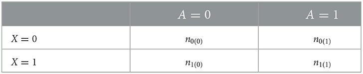
Table 1. Data table for Example 3.

The treatment effect can be derived based on Equation (7). When ${\sigma }_0^2\to 0$, then λ → 1, $\widehat{\tau }\to {\widehat{\tau }}_R$, we have

$\begin{array}{l}C1=(q_0{n}_0+q_1{n}_1)\times (q_0{n}_{0(1)}{n}_{0(0)}({\overline{Y}}_{0(1)}-{\overline{Y}}_{0(0)})\\ +q_1{n}_{1(1)}{n}_{1(0)}({\overline{Y}}_{1(1)}-{\overline{Y}}_{1(0)})),\\ D1=(q_0{n}_0+q_1{n}_1)\times \left(q_0{n}_{0(1)}{n}_{0(0)}+q_1{n}_{1(1)}{n}_{1(0)}\right)\end{array}$

We can derive

$\begin{array}{l}\widehat{\tau }=\frac{C1}{D1}\\ =\frac{n_0{\pi }_0(1-{\pi }_0)}{n_0{\pi }_0(1-{\pi }_0)+n_1{\pi }_1(1-{\pi }_1)}\widehat{\tau }(X=0)\\ +\frac{n_1{\pi }_1(1-{\pi }_1)}{n_0{\pi }_0(1-{\pi }_0)+n_1{\pi }_1(1-{\pi }_1)}\widehat{\tau }(X=1)\end{array}$

In general, for multiple levels of X, the treatment effect is a weighted average of the treatment effect τ_l = E(Y(1)−Y(0)|X = l),

$\begin{array}{l}\widehat{\tau }={\displaystyle \sum w_l\widehat{{\tau }_l}}\end{array}$

where the weight w_i is determined by the variance of Pr(A = 1|X = l) = n_lπ_l(1−π_l), with π_l = 0.5 receiving maximum possible weight. On the other hand, for the subgroup where π_l is very small or very large, they contribute very little to the overall averaged treatment effect. When there are non-ignorable noises ${\sigma }_0^2>0$, again the treatment effect is a shrinkage estimate of the weighted average of the heterogeneous treatment effects, shrinking toward the overall contrast between the treated and untreated groups.

The above demonstration was presented by considering a categorical X, with K being a block diagonal matrix of 0 and 1 s. For general types of X, the squared exponential covariance function offers a way to specify a distance matching, which closely resembles Mahalanobis distance matching. For a pair of “matched” individuals, i.e., sample units with the same set of confounding variables v_i = v_j, the model specifies $Corr(Y_i^{(0)},Y_j^{(0)})=1$. In other words, the “matched” individuals are expected to be exchangeable. As the data points move further apart in the covariate space, their correlation becomes smaller. When the distance is far apart sufficiently, the model specifies $Corr(Y_i^{(0)},Y_j^{(0)})\approx 0$ or “unmatched.” Distinct length scale parameters are used to allow for some confounders to play more important roles than others in matching. By manipulating the values of v_i and the corresponding length scale parameter, one could formulate the SE covariance matrix to reflect the known 0/1 or various degrees of matching structure. However, the matching structure is usually unknown and was left to be estimated in the model informed by the observed data. Unlike the propensity score or other distance matching method, using the GP covariance function as the matching tool provides a flexible and data-driving way of defining “similarity” between any pairs of data points, and thus offer more weights to the “similar” data points in a finer gradient.

3.2. Doubly robust property

Causal inference estimators with the doubly robust (DR) property are particularly attractive given their ability to address the dual data-generating processes underlying the causal inference problem. Multiple versions of DR causal estimators (e.g., Scharfstein et al. [29], Bang and Robins [30], and Chernozhukov et al. [31]) have been proposed. They all can be considered as a contrast between two weighted terms of treatment groups, and their DR properties are established under the conditions of the correct specification of either the outcome regression model or the propensity score. Such an argument is not straightforward within the Bayesian framework, although there have been new developments emerging that linked empirical likelihood with estimating equations for parameter estimations, as well as constructing Bayesian methods for models formulated through moment restrictions (e.g., Schennach [32], Chib et al. [33], Florens and Simoni [34], and Luo et al. [35]).

We conjecture that the GPMatch possesses the DR properties asymptotically in the following sense. Let the true average treatment effect (ATE) be τ^*, the GPMatch estimator is an unbiased estimate of the ATE when either one of the conditions is true: (i) the GP mean function $Z_i^{\prime }\gamma$ is correctly specified; or (ii) the GP covariance function is correctly specified, in the sense that, from the weight-space point of view of GP regression, the weighted sum of treatment assignment consistently estimates the true treatment propensity π_i = Pr(A = 1|X_i).

Under the condition (i), the partial linear component of the $Y_i^{(a)}=Z_i^{\prime }\gamma +f(x)$ is correctly specified, we may apply the results of Theorem 1 of Choi and Woo [24], which suggests that the posteriors of the GPMatch parameters can be consistently estimated. It follows that the averaged treatment effect can be consistently estimated.

The second condition assumes a known GP prior. We consider a simple misspecification of the form E(Y_i) = f_i(x)+A_iτ. From the weight-space point of view, given τ, the predicted value of the potential outcome from the GPMatch model can be asymptotically approximated by

$\begin{array}{ll}{\widehat{Y_i}}^{(a)}=\sum _{j=1}^n{w}_{ij}(Y_j-A_j\tau )+a\tau =\widetilde{Y_i}+(a-\widetilde{A_i})\tau ,& (8)\end{array}$

where $\widetilde{Y_i}=\sum _{j=1}^n{w}_{ij}{Y}_j$ and ${Ã}_i=\sum _{j=1}^n{w}_{ij}{A}_j$, for i = 1, ..., n. The weight $w_{ij}=\frac{{\kappa }_{ij}}{\sum _j{\kappa }_{ij}}$ where ${\kappa }_{ij}=k{(v_j)}^{\prime }{\Sigma }^{-1}$, with k(v_j) = (k(v_j, v_i))_n×1. Thus, the $\widetilde{Y_i}$ and $\widetilde{A_i}$ could be considered as the Nadaraya-Watson estimator of the observed outcomes and treatment assignment for each of the i-th unit in the sample. The estimate of treatment effect could be obtained by solving $\frac{\partial \sum _{i=1}^n{(Y_i-{\widehat{Y_i}}^{(A_i)})}^2}{\partial \tau }=0$. We can see that, given a known GP covariance function, the GPMatch treatment effect $\widehat{\tau }$ is an M-estimator satisfies $\sum {\text{Ψ}}_i(\widehat{\tau })=0$, where

$\begin{array}{ll}{\Psi }_i(\tau )=\left(Y_i-\widetilde{Y_i}-\tau (A_i-{\tilde{A}}_i)\right)(A_i-{\tilde{A}}_i),& (9)\end{array}$

Let the true propensity be π_i = Pr(A = 1|X_i), given the SUTVEA, we have $Y_i=A_i{Y}_i^{(1)}+(1-A_i)Y_i^{(0)}+{ϵ}_i$. Given the true treatment effect τ^*, we can write $Y_i^{(a)}=E(Y_i)+(a-{\pi }_i){\tau }^{*}$. Thus, when $\widetilde{A_i}={\pi }_i$ asymptotically, we have ${\text{Ψ}}_i(\tau )=\left[E(Y_i)-\widetilde{Y_i}+(A_i-{\pi }_i)(\tau -{\tau }^{*})+{ϵ}_i\right](A_i-{\pi }_i)$. It follows the estimating function is conditionally unbiased, i.e., $E({\text{Ψ}}_i({\tau }^{*}))=0$, for i = 1, ...n.

Remark 1. First, the Equation (9) is the empirical correlation of the residuals from the outcome model and the residuals from the propensity of treatment assignment. Thus, GPMatch attempts to induce independence between the treatment selection process and the outcome modeling, just as the G-estimation equation does (see Robins et al. [36] and Vansteelandt and Joffe [37]). Unlike the moment-based G-estimator, which requires the fitting of two separate models for the outcome and propensity score, the GPMatch approach estimates covariance parameters at the same time as it estimates the treatment and mean function parameters. All within a full Bayesian likelihood framework.

Second, some data points may have a treatment propensity close to 0 or 1. Those data usually are a cause of concern in causal inference. In the naive regression type of model such as BART, it may cause unstable estimation without added regularization. In the inverse probability treatment weighting type of method, a few data points may put undue influence over the estimation of treatment effect. In matching methods, these data points often are discarded. Such practice could lead to the sample no longer being representative of the target population. Like the G-estimation, we can see from the Equation (9), these data points contribute very little or no information to the GPMatch estimation of the treatment effect. Thus GPMatch shares the same added robustness as the G-estimation.

Third, the GPMatch model with a parametric mean function can be used in predicting the potential outcomes for any new unit, by $\widehat{Y_i}=Z_i^{\prime }\widehat{\gamma }+{\Sigma }_i{\Sigma }^{-1}(Y_n-Z\widehat{\gamma })$, where Σ_i denotes the i-th row of Σ. Given the model setup, two regression surfaces are predicted, where the distance between the two regression surfaces represents the treatment effect. By including the treatment by covariate interactions, the model could offer estimates of conditional averaged treatment effects for pre-specified patient characteristics.

Finally, in real-world applications, we may never know the true functional form of neither the mean nor the covariance function. The only exception is the designed experimental study, where propensity scores are known. When the true propensity score is known, it can be directly used for specifying GP prior. With high dimensional X, we may wish to reduce dimensions first. One approach is to estimate summary scores, such as the estimated propensity score. Another approach is to engage variable selection procedures. As in the propensity-score-based methods, we wish to design the covariance function to ensure covariate balance between the treatment groups. Given the fitted ${{M}}_{GPMatch}$ model, covariate balance can be diagnosed by comparing weighted samples of $\left[X|A=0,{{M}}_{GPMatch}\right]$ and $\left[X|A=1,{{M}}_{GPMatch}\right]$ (see an example in Huang et al. [38]).

4. Simulation studies

To empirically evaluate the performances of GPMatch in a real-world setting where neither the matching structure nor the functional form of the outcome model are known, we conducted four sets of simulation studies to evaluate the performances of the GPMatch approach to causal inference. The first set evaluated the frequentist performance of GPMatch. The second set compared the performance of GPMatch against MD match, the third set considered a setting with a large number of correleted background variables where only a few are relevant to the data generating mechanisms and the last set utilized the widely used Kang and Schafer design, comparing the performance of GPMatch against some commonly used propensity methods as well as the nonparametric Bayesian additive regression tree (BART) method.

In all simulation studies, the GPMatch approach used a squared exponential covariate function, including only the treatment indicator in the mean and all observed covariates into the covariance function, unless otherwise noted. The results were compared with the following widely used causal inference methods: sub-classification by PS quantile (QNT-PS); augmented inverse probability of treatment weighting (AIPTW), a linear model with PS adjustment (LM-PS), a linear model with spline fit PS adjustment [LM-sp(PS)] and BART. Cubic B-splines with knots based on quantiles of PS were used for LM-sp(PS). We also considered the direct linear regression model (LM) as a comparison. The ATE estimates were obtained by averaging over 5000 posterior MCMC draws, after 5,000 burn-in. For each scenario, three sample sizes were considered, N = 100, 200, and 400. The standard error and the 95% symmetric interval estimate of ATE for each replicate were calculated from the 5,000 MCMC chain. For comparing performances of different methods, all results were summarized over N = 100 replicates by the root mean square error RMSE $=\sqrt{\sum {({\widehat{\tau }}_i-\tau )}^2/N}$, median absolute error MAE $=median\mid {\widehat{\tau }}_i-\tau \mid$, coverage rate Rc = (the number of intervals that include τ)/N of the 95% symmetric posterior interval, the averaged standard error estimate $S{E}_{ave}=\sum {\widehat{\sigma }}_i/N$, where ${\widehat{\sigma }}_i$ is the square root of the estimated standard deviation of ${\widehat{\tau }}_i$, and the standard error of ATE was calculated from 100 replicates $S{E}_{emp}=\sqrt{\sum {({\widehat{\tau }}_i-\overline{\widehat{{\tau }_i}})}^2/(N-1)}$.

4.1. Well-calibrated frequentist performances

Let the single covariate x~N(0, 1). The potential outcome was generated by $y^{(a)}=e^x+(1+U)\times a+U_0$ for a = 0, 1, where the true treatment effect was 1+U_i for the i-th individual unit. The (U, U₀) are unobserved covariates. The treatment was selected for each individual following logit(P(A = 1|X)) = −0.2+(1.8X)^1/3. The observed outcome was generated by $y|x,a~N(y^{(a)},{\sigma }_0^2)$. Two parameter settings were considered. First, we set $\left\{U_i=0,U_{0i}~N(0,0.25),{\sigma }_0^2=0.75\right\}$, i.e., all individual units had the same uniform treatment effect of 1, and outcomes were observed with measurement error. Second, we set $\left\{U_i~N(0,0.15^2),U_{0i}~N(0,1),{\sigma }_0^2=0\right\}$, i.e., the treatment effect varied from individual unit to unit, but the averaged treatment effect remained at 1.

The simulation results were summarized in the histogram of the posterior mean over the 100 replicates across three sample sizes in Figure 1. Table 2 presented the results of GPMatch and the Oracle standard. The Oracle estimate was obtained by fitting the true outcome-generating model for benchmark. For both Figure 1 and Table 2, the upper panel presented results from the uniform treatment parameter setting, and the lower panel presented the results from the homogeneous treatment setting. Under both settings, GPMatch presented well-calibrated frequentist properties with nominal coverage rate, and only slightly larger RMSE. The averaged bias, RMSE, and MAE quickly improve as sample size increases, and its performance is almost as well as the Oracle with a sample size of 400.

FIGURE 1

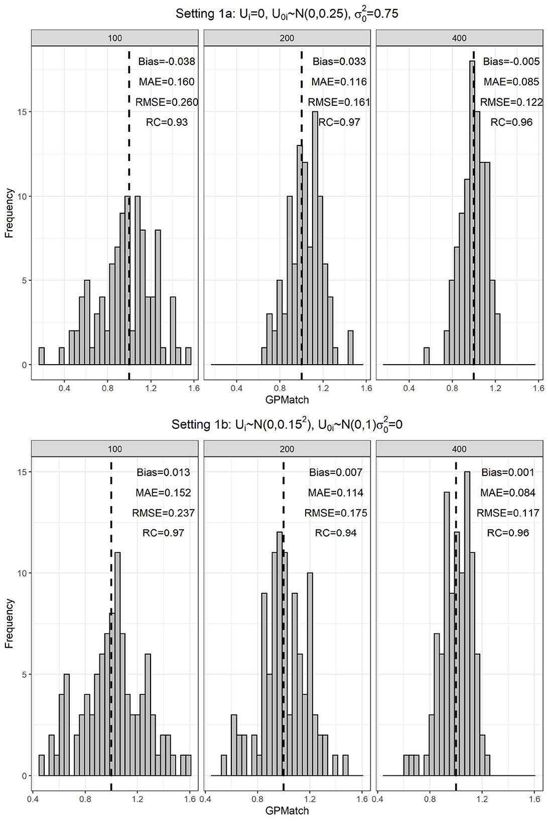
Figure 1. Distribution of the GPMatch estimate of ATE, by different sample sizes under the single covariate simulation study setting.

TABLE 2

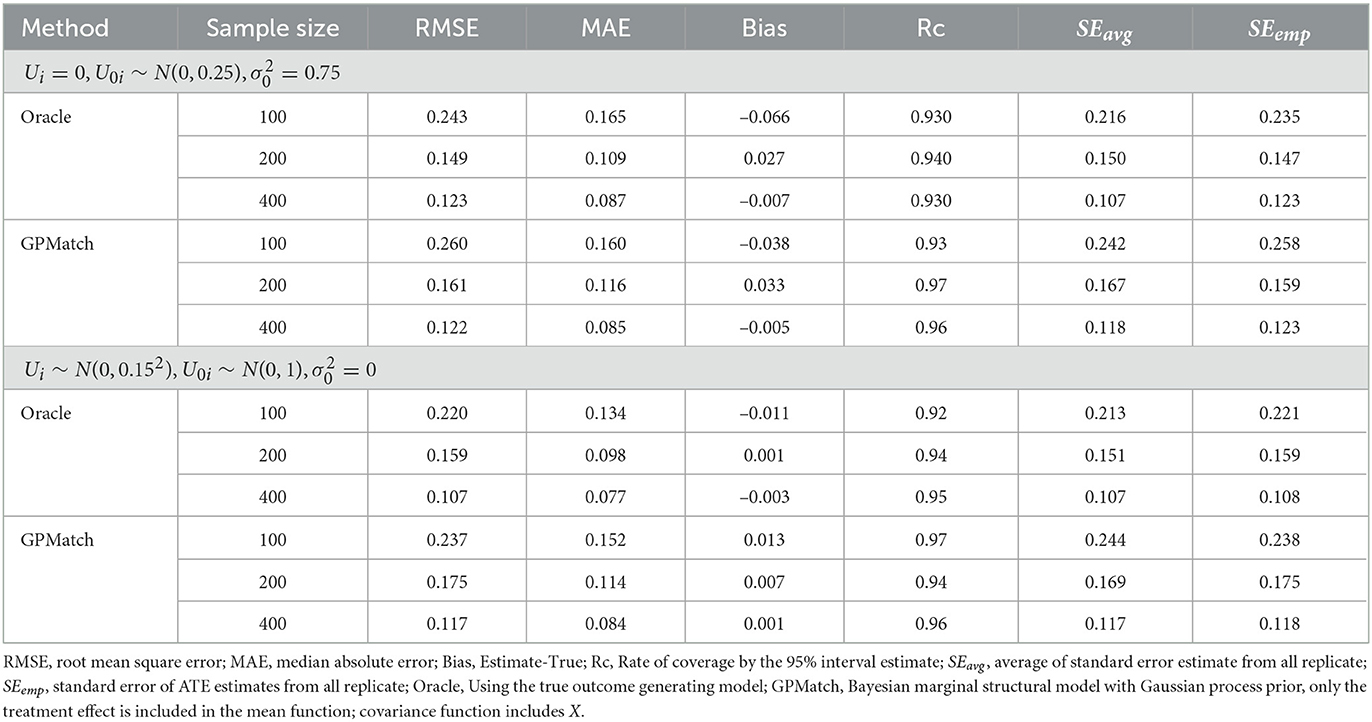
Table 2. Results of ATE estimates under the single covariate simulation study setting.

We also applied some commonly adopted causal inference methods as well as the BART to the simulated data. Their performances are presented as the %bias, the ratio of RMSE and MAE in reference to the oracle results in Figure 2. The results show that the impact of measurement error varies by the method, whether the propensity score is correctly estimated, as well as the sample sizes. At sample size 100, even with correctly specified PS, the %bias ranges from 5 to 10% for PS-based methods, and the MAE and RMSE are at least 1.5 times the oracle estimates. Their performances improve with increased sample size if the propensity score is correctly specified. However, when the propensity score is miss-specified, the performance could get even worse with an increased sample size. Of all PS-based methods, flexible modeling LM-sp(PS) using spline fit of PS appears to perform the best. The two Bayesian flexible modeling techniques, BART and GP had the best performances w.r.t. MAE and RMSE, with BART performing nearly as well as GP when the sample size is N = 400. However, the %bias results from BART presented surprisingly larger %bias for N = 200 than N = 100. These results suggest that not explicitly acknowledging measurement error, the existing methods may suffer from bias.

FIGURE 2

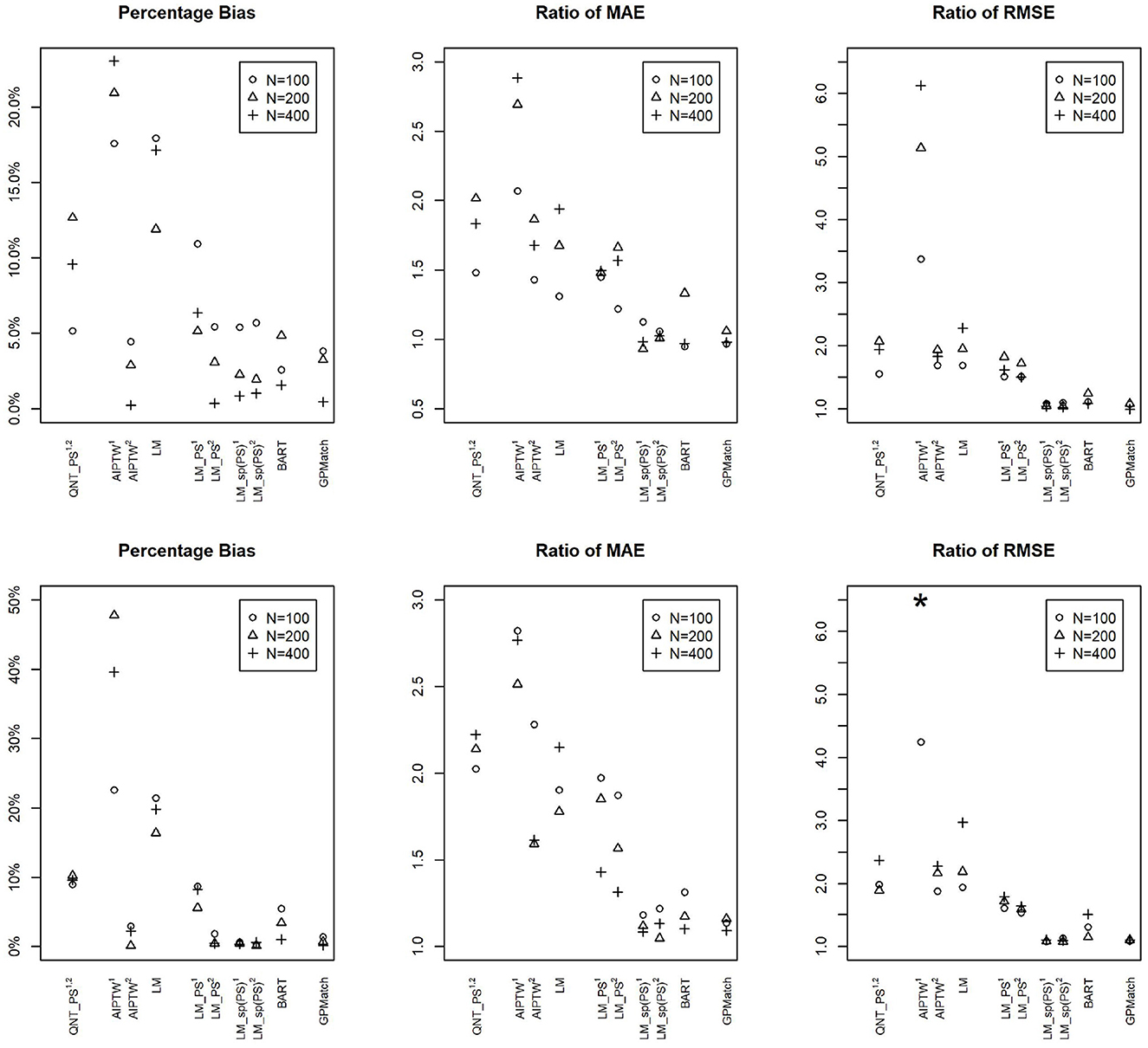
Figure 2. Comparisons of percentage bias, root mean square error (RMSE), and median absolute error (MAE) of the ATE Estimates by Different Methods Across Different Sample Sizes under the Simulation Setting 1a (upper panel): $U_i=0,U_{0i}~N(0,0.25),{\sigma }_0^2=0.75$ and Setting 1b (lower panel): $U_i~N(0,0.15^2),U_{0i}~N(0,1),{\sigma }_0^2=0$. ¹Propensity score estimated using logistic regression on logitA ~ X. ²Propensity score estimated using logistic regression on logitA ~ X^1/3. GPMatch, Bayesian structural model with Gaussian process prior; QNT_PS, Propensity score sub-classification by quintiles; AIPTW, augmented inversed probability of treatment weighting; LM, linear regression modeling Y ~ X; LM_PS, linear regression modeling with propensity score adjustment; LM_sp(PS), linear regression modeling with spline fit propensity score adjustment. BART, Bayesian additive regression tree. *The ratios of RMSE of N = 200 and N = 400 for AIPTW¹ are 24.23 and 11.68 which are truncated.

4.2. Compared to Mahalanobis distance matching

To compare the performances between the MD matching and GPMatch, we considered a simulation study with two independent covariates x₁, x₂ from the uniform distribution U(−2, 2), treatment was assigned by letting A_i~Ber(π_i), where

$\begin{array}{l}logit{\pi }_i=-x_1-x_2.\end{array}$

The potential outcomes were generated by

$\begin{array}{l}{y}_i^{(a)}=3+5a+x_{1i}^3,\end{array}$

$\begin{array}{l}{Y}_i|X_i,A_i~N(y_i^{(A_i)},1).\end{array}$

The true treatment effect is 5. Three different sample sizes were considered N = 100, 200, and 400. For each setting, 100 replicates were performed and the results were summarized.

We estimated ATE by applying Mahalanobis distance matching and GPMatch. The MD matching considered caliper varied from 0.125 to 1 with step size 0.025, including both X₁ and X₂ in the matching using the function Match in R package Matching by Sekhon [39]. The averaged bias and its 95%-tile and 5%-tile were presented as vertical lines corresponding to different calipers in Figure 3. To be directly comparable to the matching approach, the GPMatch estimated the ATE by including the treatment effect only in modeling the mean function, both X₁ and X₂ were considered in the covariance function modeling. The posterior results were generated with 5,000 MCMC samples after 5,000 burn-in. Its averaged bias (short dashed horizontal line) and 5 and 95%-tiles of the ATE estimate (long dashed horizontal lines) are presented in Figure 3 for each of the sample sizes. Also presented in the figure are the bias, median absolute error (MAE), root mean square error (RMSE), and rate of coverage rate (Rc) summarized over 100 replicates of GPMatch. The bias from the matching method increases with the caliper; the width of the interval estimate varies by sample size and caliper. It reduces with increased caliper for a sample size of 100, but increases with increased caliper for a sample size of 400. In contrast, GPMatch produced a much more accurate and efficient estimate of ATE for all sample sizes, with an unbiased ATE estimate and nominal coverage rate. The 5 and 95%-tiles of ATE estimates are always smaller than those from the matching methods for all settings considered, suggesting better efficiency of GPMatch.

FIGURE 3

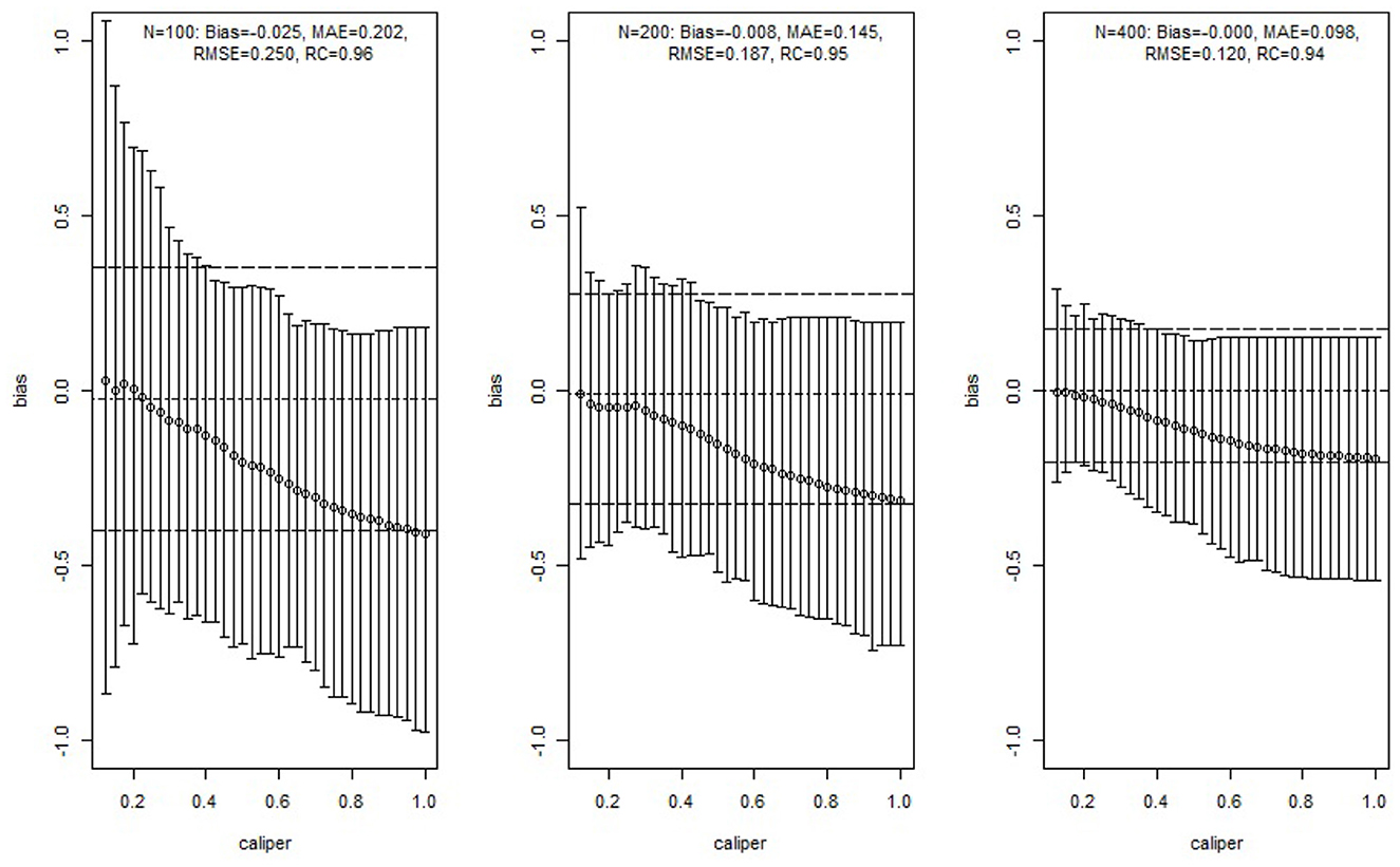
Figure 3. Simulation study results of comparing GPMatch with Mahalanobis distance matching methods. The circles are the averaged biases of estimates of ATE using Mahalanobis matching with corresponding calipers. The corresponding vertical lines indicate the ranges between the 5th and 95th percentiles of the biases. The horizontal lines are the averaged ATE (short dashed line), and the 5th percentile and 95th percentile (long dashed line) of the biases of the estimates from GPMatch.

4.3. High dimension covariates

The background covariates could be of high dimension. While the GP prior could include high dimensional X, the computational burden can be too demanding. To address the issue, we considered two-dimensional reduction strategies. First, we use the estimated propensity score in constructing the GP covariance function, where the PS is obtained by a logistic regression on all covariates. Second, we engaged a standard stepwise selection procedure for the logistic regression modeling of treatment selection prior to the GP modeling, where only selected variables are included in the GP covariance function. Here, we simply used the default setting of the variable selection procedure implemented in the standard R step function. At last, for comparison, we generated the propensity score using the true logistic model.

Modified from the simulation setting presented in Section 4.2, we considered 25 dependent covariates X₁, ..., X₂₅ generated from a multivariate normal distribution with mean 0, variance 1, and the correlation $Corr(X_i,X_j)=0.5^{|i-j|}$. The treatment A_i was generated from a Bernoulli distribution with probability π_i, where

$\begin{array}{l}logit({\pi }_i)=-x_{1i}-x_{2i}.\end{array}$

The potential outcomes were generated by

$\begin{array}{l}{y}_i^{(a)}=3+5a+x_{1i}^3+2x_{3i},\end{array}$

$\begin{array}{l}{Y}_i|X_i,A_i~N(y_i^{(A_i)},1).\end{array}$

The true treatment effect is 5. We considered three different sample sizes: N = 100, 200, and 400. For each setting, 100 replicates were performed and the results were summarized. For comparison, we applied the Mahalanobis distance matching method using all X₁−X₂₅ and using only the true covariate set (X₁, X₂). The MD match considered caliper varied from 0.125 to 1 with step size 0.025. Same as Section 4.2, the Match function from the R package Matching is used.

The comparisons of MAE and RMSE of these methods are shown in Figure 4. Without variable selection, both MD match and GPMatch presented large biases for the sample size of 100. The performance quickly improves as the sample size increases for GPMatch, but not so for the MD match. The variable selection procedure clearly enhanced the performance for GP, with results indistinguishable from those using the true PS when N = 400. GPMatch results are identical between the model with a true covariate set and the model with true PS.

FIGURE 4

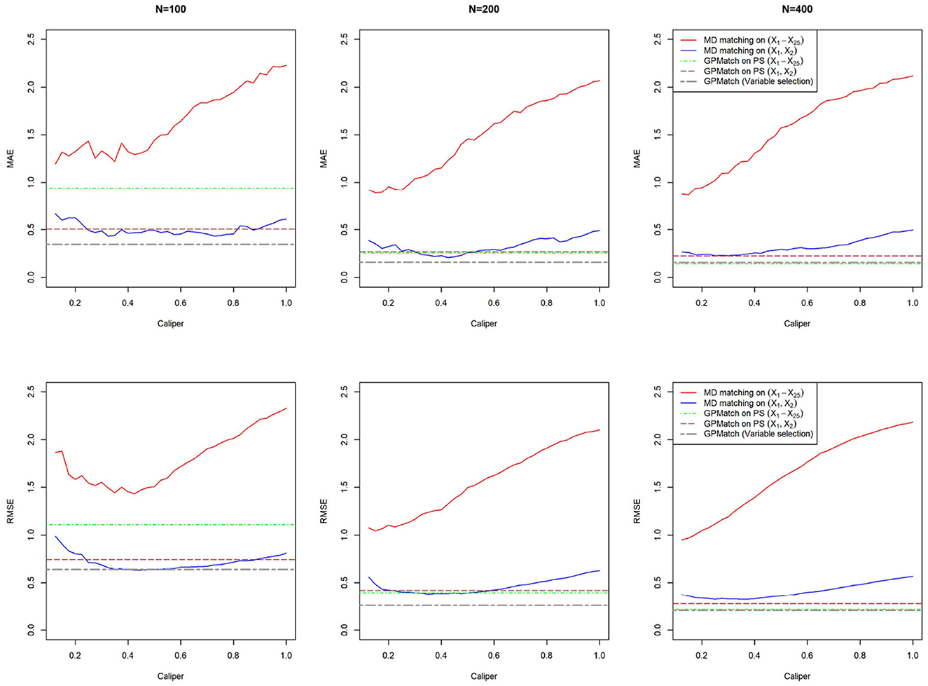
Figure 4. Comparison of MAE and RMSE of Mahalanobis and GPMatch methods.

4.4. Performance under dual misspecification

Following the well-known simulation design suggested by Kang and Schafer [27], covariates z₁, z₂, z₃, z₄ were independently generated from the standard normal distribution N(0, 1). Treatment was assigned by A_i~Ber(π_i), where

$\begin{array}{l}logit{\pi }_i=-z_{i1}+0.5z_{i2}-0.25z_{i3}-0.1z_{i4}.\end{array}$

The potential outcomes were generated for a = 0, 1 by

$\begin{array}{l}{y}_i^{(a)}=210+5a+27.4z_{i1}+13.7z_{i2}+13.7z_{i3}+13.7z_{i4},\end{array}$

$\begin{array}{l}{Y}_i|A_i,X_i~N(y^{(A_i)},1).\end{array}$

The true treatment effect is 5. To assess the performances of the methods under the dual misspecifications, the transformed covariates $x_1=exp(z_1/2),x_2=z_2/(1+exp(z_1))+10,x_3={(\frac{z_1{z}_3}{25}+0.6)}^3$, and $x_4={(z_2+z_4+20)}^2$ were used in the model instead of z_i.

Two GPMatch models were considered: GPMatch1 modeled the treatment effect only and GPMatch2 modeled all four covariates X₁−X₄ in the mean function model. Both included X₁−X₄ with four distinct length scale parameters. The PS was estimated using two approaches including the logistic regression model on X₁−X₄ and the covariate balancing propensity score method (CBPS, [40]) applied to X₁−X₄. The results corresponding to both versions of PS were presented. Summaries over all replicates were presented in Table 3, and the RMSE and the MAE were plotted in Figure 5, for all methods considered. As a comparison, the Oracle uses the true outcome generating model of Y~Z₁−Z₄ was also presented. Both GPMatch1 and GPMatch2 clearly outperform all the other causal inference methods in terms of bias, RMSE, MAE, Rc, and the SE_ave is closely matched to SE_emp. The ATE and the corresponding SE estimates improve quickly as the sample size increases for GPMatch. In contrast, the QNT_PS, AIPT, LM_PS, and LM_sp(PS) methods show little improvement over increased sample size, nor does the simple LM. Improvements in the performance of GPMatch over existing methods are clearly evident, with more than 5 times accuracy in RMSE and MAE compared to all the other methods except for BART. Even compared to the BART results, the improvement in MAE is nearly twice for GPMatch2 and about 1.5 times for GPMatch1. Similar results are evident in RMSE and averaged bias. The lower-than-nominal coverage rate is mainly driven by the remaining bias, which quickly reduces as the sample size increases. Additional results are presented in Supplementary Figure S1.

TABLE 3

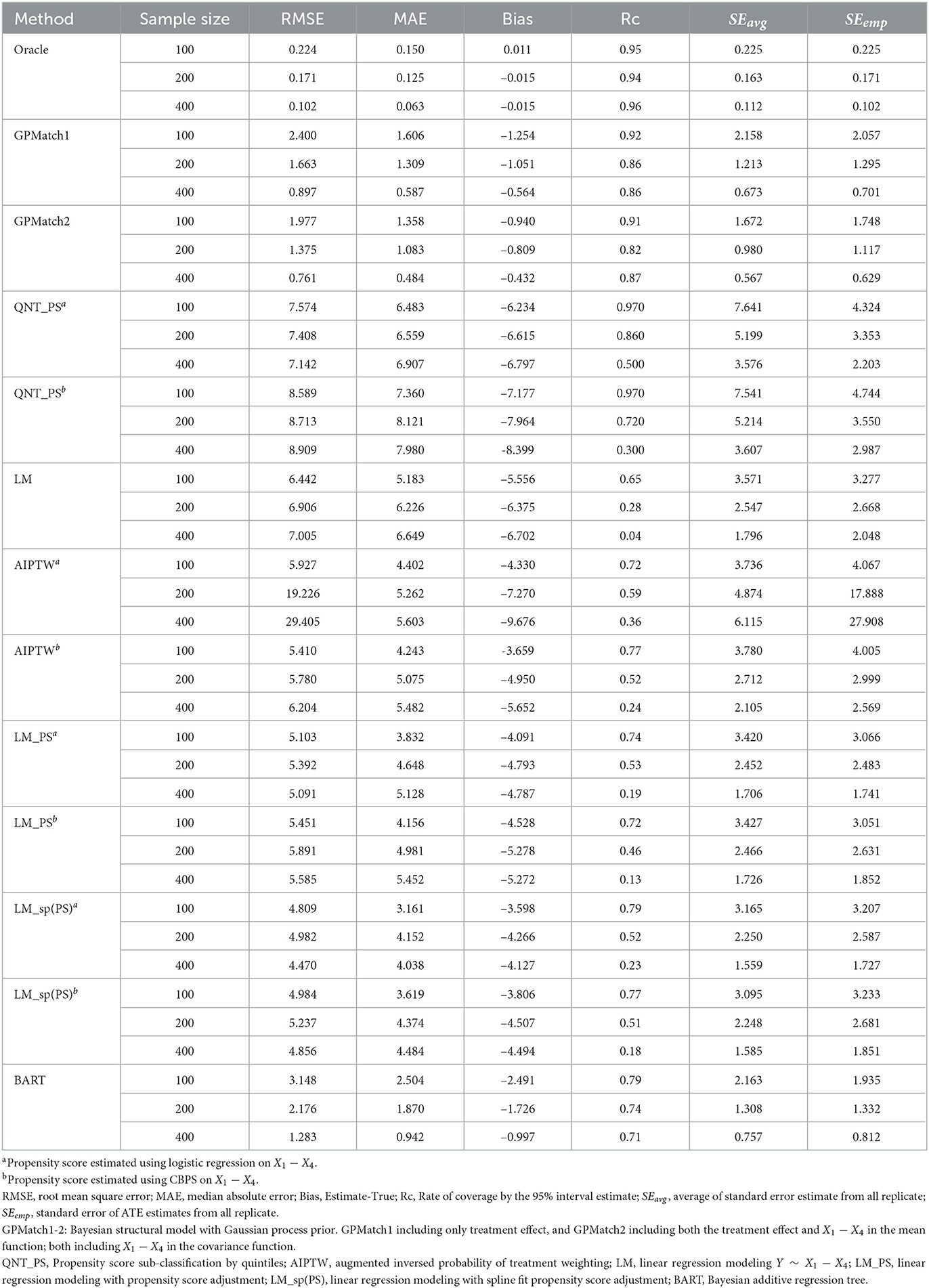
Table 3. Results of ATE estimates using different methods under the Kang and Shafer dual misspecification setting.

FIGURE 5

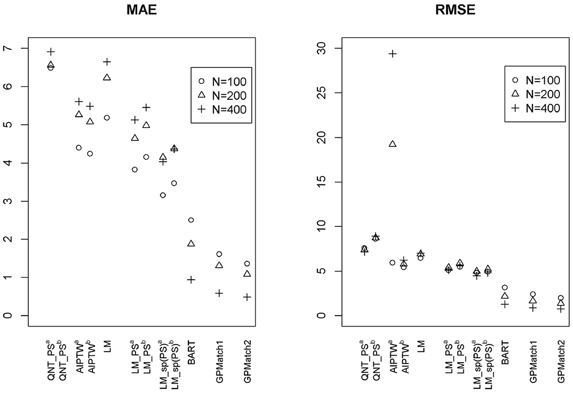
Figure 5. The RMSE and MAE of ATE Estimates using Different Methods under the Kang and Shafer Simulation Study Setting. GPMatch1-2: Bayesian structural model with Gaussian Process prior. GPMatch1 including only the treatment effect, and GPMatch2 including both the treatment effect and X₁ − X₄ in the mean function; and X₁ − X₄ are included in the covariance function. QNT_PS, Propensity score sub-classification by quintiles; AIPTW, augmented inverse probability of treatment weighting; LM, linear regression modeling Y ~ X₁ − X₄; LM_PS, linear regression modeling with propensity score adjustment; LM_sp(PS), linear regression modeling with spline fit propensity score adjustment.

5. A case study

JIA is a chronic inflammatory disease, the most common autoimmune disease affecting the musculoskeletal organ system, and a major cause of childhood disability. The disease is relatively rare, with an estimated incidence rate of 12 per 100,000 child-year [41]. There are many treatment options. Currently, the two common approaches are the non-biologic disease-modifying anti-rheumatic drugs (DMARDs) and the biological DMARDs. Limited clinical evidence suggests that early aggressive use of biologic DMARDs may be more effective [42]. Utilizing data collected from a completed prospectively followed-up inception cohort research study [43], a retrospective chart review collected medication prescription records for study participants captured in the electronic health record system. This comparative study is aimed at understanding whether therapy using an early aggressive combination of non-biologic and biologic DMARDs is more effective than the more commonly adopted non-biologic DMARDs monotherapy in treating children with recently (less than 6 months) diagnosed polyarticular course of JIA. The study is approved by the investigator's institutional IRB.

The primary outcome is the Juvenile Arthritis Disease Activity Score (JADAS) after 6 months of treatment, a disease severity score calculated as the sum of four core clinical measures: physician's global assessment of disease activity (0–10), patient's self-assessment of overall wellbeing (0–10), erythrocyte sedimentation rate (ESR, standardized to 0–10), and number of active joint counts (AJC, truncated to 0–10). It ranges from 0 to 40, with 0 indicating no disease activity. Out of the 75 patients receiving either non-biological or the early combination of biological and non-biological DMARDs at baseline, 52 patients were treated by the non-biologic DMARDs and 23 were treated by the early aggressive combination DMARDs. The patients with longer disease duration, positive rheumatoid factor (RF) presence, higher pain visual analog scale (VAS) and lower baseline functional ability as measured by the childhood health assessment questionnaire (CHAQ), higher lost range of motion (LROM) and JADAS score are more likely to receive the biologic DMARDs prescription. The propensity score was derived using the CBPS method applied to the 11 pre-determined important baseline confounders. The derived PS was able to achieve the desired covariate balance within the 0.2 absolute standardized mean difference (Figure 6).

FIGURE 6

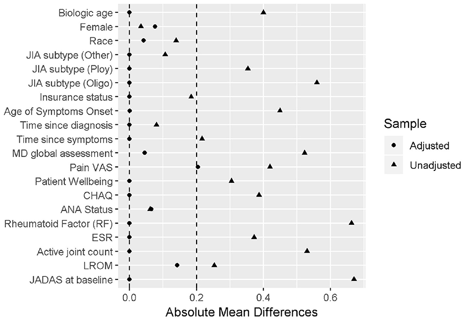
Figure 6. Balance check results for the cases study.

We considered two GPMatch modeling approaches. The first included the full list of covariates. The second only included variables selected from the step-wise logistic regression modeling of treatment assignment. The following five variables: baseline JADAS, CHAQ, time since diagnosis, positive test of rheumatoid factor, and private insurance are selected. These five covariates, along with the binary treatment indicator, time of the 6-month follow-up since baseline were used in the partially linear mean function part of the GPMatch. For comparisons, PS methods also considered two corresponding sets of covariates in the outcome modeling when applicable. The results are presented in Table 4 with the left panel presenting results using selected covariates, and the right panel presenting the results including the full set of covariates. With including selected variables, GPMatch obtained the average treatment effect of –2.98 with standard error of 1.99, and the 95% credible interval of (–6.91, 0.83). The results differs by < 0.5 point comparing the point estimates of two GPMatch models. The results are also similar for other PS-based methods, with BART showing more sensitivity to choices of covariates. Figure 7 presents the trace plot and histogram of the posterior distribution of the ATE estimate. The results suggest that the early aggressive combination of non-biologic and biologic DMARDs as the first line of treatment is more effective, leading to a nearly 3-point reduction in JADAS 6 months after treatment, compared to the non-biologic DMARDs treatment in children with a newly diagnosed disease. The results of ATE estimates by GPMatch, naive two-group comparison, and other existing causal inference methods are presented in Table 4. The LM, LM_PS, LM_sp(PS), and AIPTW include the same five covariates in the model along with the treatment indicator. BART used the treatment indicator and those covariates. While all results suggested the effectiveness of early aggressive use of biological DMARD, the naive, PS sub-classification by quintiles, and AIPTW suggested a much smaller ATE effect. The BART and PS adjusted linear regression produced results that were closer to the GPMatch results suggesting a 2 or 3 points reduction in the JADAS score if treated by the early aggressive combination DMARDs therapy. None of the results were statistically significant at the 2-sided 0.05 level.

TABLE 4

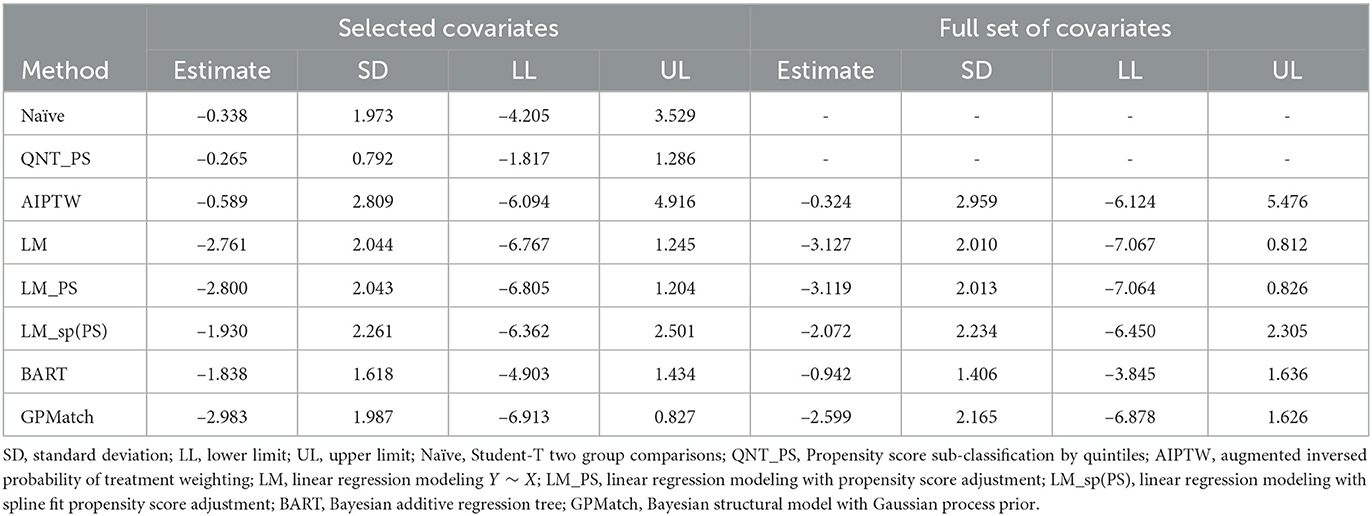
Table 4. Results of case study ATE estimates with none-matching methods.

FIGURE 7

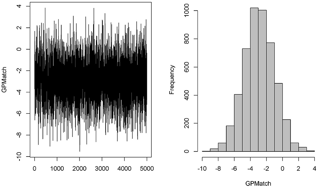
Figure 7. Case study trace plot and histogram.

We also applied the covariate matching method to the same dataset based on the same five baseline covariates. Table 5 presents the results from using different calipers. As expected, as calipers narrow, the number of observations being discarded increases. Since only 10 patients had RF positive when the calipers ≤ 0.5, we cannot matching on RF positive anymore. Similarly, because of distributions of private insurance in the treated and untreated groups, we cannot match on the insurance when the caliper was set to 1 or smaller. Thus, for calipers ≤ 1, all subjects with private insurance were being excluded. When calipers were ≤ 0.5, all subjects with positive RF were excluded, and 50% of observations were discarded. When the calipers were set at 0.2, 67 out of 75 observations were discarded, rendering the results obtained from 8 observations only! The estimate of ATE was sensitive to the choices of calipers, which ranged from –2.0 to –4.28, making it difficult to interpret the study results.

TABLE 5

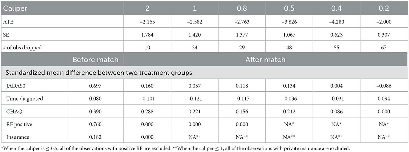
Table 5. Results of case study ATE estimates with matching method in case study.

6. Conclusions and discussions

Bayesian approaches to causal inference commonly consider it as a missing data problem. However, as suggested in Ding and Li [44], the causal inference presents additional challenges that are unique in itself other than the missing data alone. Approaches not carefully address these unique challenges are vulnerable to model misspecifications and could lead to seriously biased results. When not considering the treatment-by-indication confounding, naive Bayesian regression approaches could suffer from “regularity induced bias” [11]. Because no more than one potential outcome could be observed for a given individual unit, the correlation of $(Y_i^{(1)},Y_i^{(0)})$ is not directly identifiable, leading to “inferential quandary” [45]. Extensive simulations [23, 27, 46] suggested poor operational characteristics observed in many widely adopted causal inference methods.

The proposed GPMatch method offers a full Bayesian causal inference approach that can effectively address the unique challenges inherent in causal inference. First, utilizing GP prior covariance function to model the covariance of observed data, GPMatch could estimate the missing potential outcomes much like the matching method. Yet, it avoids the pitfalls of many matching methods. No data is discarded, and no arbitrary caliper is required. Instead, the model allows the data to speak by itself via estimating length scale and variance parameters. The SE covariance function of GP prior offers an alternative distance metric, which closely resembles Mahalanobis distance. It matches data points by the degree of matching proportional to the SE distance, without requiring the specification of a caliper. For this reason, the GPMatch could utilize data information better than the matching procedure. Different length scale parameters are considered for different covariates used in defining the SE covariance function. This allows the data to select the most important covariates to be matched on, and acknowledge some variable is more important than others. While the idea of using GP prior to Bayesian causal inference is not new. Utilizing the GP covariance function as a matching device is a unique contribution of this study. The matching utility of the GP covariance function is presented analytically. We presented a heuristic argument suggesting GPMatch possesses doubly robust properties asymptotically. We show that GPMatch estimates the treatment effect by inducing independence between two residuals: the residual from the treatment propensity estimate and the residual from the outcome estimate, much like the G-estimation method. Unlike the two-staged G-estimation, the estimations of the parameters in the covariance function and the mean function for the GPMatch are performed simultaneously. Therefore, the GPMatch regression approach can integrate the benefits of the regression model and matching method and offers a natural way for Bayesian causal inference to address challenges unique to the causal inference problems. The robust and efficient proprieties of GPMatch are well supported by the simulation results designed to reflect the most realistic settings, i.e., no knowledge of matching or functional form of outcome model is available.

The validity of the causal inference by the GPMatch approach rests on three causal assumptions. In particular, we propose SUTVEA as a weak causal assumption than SUTVA. SUTVEA suggests that the potential outcomes and their difference are random variables. It can be considered as a version of the stochastic consistency advocated by Cole and Frangakis [47] and VanderWeele [48]. The SUTVEA is proposed to reflect a more realistic setting that the outcome could be measured with error, and the treatment received by different individuals may vary, even though the treatment prescribed is identical. Despite the fact that such treatment variations were raised [1], no approach to our knowledge has explicitly acknowledged it as such. Rather, most of the methods consider the treatment from the real world as having the exactly same meaning as those from the randomized and strictly controlled experiments. Acknowledging the existence of random error in outcome measures, the GPMatch method is more capable of defending against potential model misspecification in a challenging real-world setting. Like others, the no unmeasured confounder is also required. Because no one has more than one potential outcome observed in the real world, the assumptions remain untestable. However, our SUTVEA implies the correlations among the potential outcomes have an inherent structure, which could be modeled when all confounders are observed. Therefore, potential outcomes from different individuals could be correlated. The correlation is null only when conditional on confounders. This new causal assumption allows for a direct and explicit way of describing the underlying data-generating mechanisms, which may help relieve the “inferential quandary.” By explicitly modeling the mean and covariance functions, the GPMatch can be considered an extension of the widely adopted marginal structural mean model.

The heterogeneous treatment effect (HTE) is ubiquitous. Here, we focused on presenting GPMatch for estimating the average treatment effect. We showed that the GPMatch presented a shrinkage estimate of ATE, where the shrinkage factor is determined by the variance unaccounted by the model and/or unadjusted covariates. When the observed outcome is a perfect representation of a potential outcome, i.e., when Y_i = Y_i(1)A_i+Y_i(0)(1−A_i), the GPMatch estimates ATE as a weighted average of HTEs, where the weight is determined by the propensity of treatment. The HTE strata with an equal chance of receiving either of the treatments receives the maximum possible weight, while the strata with a very small or large probability of receiving one of the treatments will be given near zero weight. This is different from the common approach of ATE, which assigns equal weight to every HTE strata. Rather, it is closely related to the concept of average treatment effect in the overlap (ATO, [49]). As such, it avoids the lack of overlapping issue, which has plagued many flexible modeling approaches to causal inference. The GPMatch can be readily used for estimating conditional averaged treatment effect (CATE) by including interactions of the pre-specified treatment modifying factors with treatment interaction. When uncertain with the treatment effect modifiers, Sivaganesan et al. [50] suggested a Bayesian decision theory-based approach for identifying subgroup treatment effects in a randomized trial setting. With GPMatch, the same idea could be applied to identify subgroup treatment by analyzing real-world data. Future studies may consider evaluating GPMatch performances for estimating heterogeneous treatment effects.

The full Bayesian modeling approach is particularly useful in comparative effectiveness research. It offers a coherent and flexible framework for incorporating prior knowledge and synthesizing information from different sources. As a full Bayesian causal inference model, the GPMatch offers a very flexible and general approach to address more complex data types and structures natural to many causal inference problem settings. It can be directly extended to consider multilevel or cluster data structure and to accommodate complex types of treatment such as multiple-level treatments, and continuous or composite types of treatment. The model could be extended to time-varying treatment settings without much difficulty by following the g-formula framework, e.g., Huang et al. [38, 51].

For the simplicity of exposition, we have considered a relatively simple setting considering binary treatment and a Gaussian outcome. The GPMatch can easily accommodate multi-level treatment, continuous and general types of treatment. The GP regression has been extended to general types of outcomes including binary and count data [52]. Future studies may further investigate its performance under the general types of treatment, outcome, and data structures. Our simulation focused on comparing with the commonly used causal inference method. Future studies may consider comparisons of our method with other advanced Bayesian methods such as those proposed by Roy et al. [10] and Saarela et al. [18], as well as other advanced non-Bayesian approaches such as TMLE [53]. At last, while our discussion has been focused on the estimation averaged treatment effect (ATE) of the sample, the approach is directly applicable to the estimation of population-averaged treatment effect, averaged treatment effect in treated and in control.

The GP regression is a very flexible modeling technique, but it is computationally expensive. The time cost associated with GP regression increases at n³ rate, thus it can be challenging with large N and/or large P. The Bayesian Gibbs Sampling algorithm we have used makes it even more demanding in computational resources. Some literature has offered solutions by applying GP to large N, such as Banerjee et al. [54]. Alternatively, one may consider using Bayesian Kernel regression as an approximation. Further studies are needed to improve the computational efficiency and to consider variable selection. We presented two dimension reduction strategies: (a) using estimate propensity score; and (b) engaging a variable selection procedure. The simulation studies have shown variable selection strategies can be promising. Alternatively, one may consider strategies specifying priors for length scale parameters. It is well known the length scale parameter is hard to estimate. Researchers derived different kinds of priors for GP, for example, the objective prior in Berger et al. [55], Kazianka and Pilz [56], and Ren et al. [57]. Gelfand et al. [58] suggested using a uniform prior for the inverse of the scale parameter in spatial analysis, but we found that using a prior with a preference to a smooth surface was more suitable for our purpose. Researchers could also blend their knowledge in the prior to obtain a more efficient estimate. Here we considered the squared exponential covariance function but different covariance functions such as Matérn could also be considered. Simple block compound symmetry with one correlation coefficient parameter could be used as an alternative covariance matrix. Such blocked covariance setup could be useful, particularly for a large sample size and where the data has a reasonable clustering structure, such as in the case of a multi-site study. Future study should explore this direction. Last, implementation of the GPMatch for causal inference may not be accessible to most practitioners. for this reason we provided an easy-to-use publicly available on-line application that allows for user supplied data. Complete step-by-step user's guide and more technical details of this and extended work can be found in our published technical report [51].

Data availability statement

The data analyzed in this study is subject to the following licenses/restrictions: Data are available on reasonable request. Requests to access these datasets should be directed to bin.huang@cchmc.org.

Ethics statement

The study was approved by the Institutional Review Board at the Cincinnati Children's Hospital Medical Center (IRB # 2015-2873). Ethical review and approval was not required for the study on human participants in accordance with the local legislation and institutional requirements. Written informed consent from the participants was not required to participate in this study in accordance with the national legislation and the institutional requirements.

Author contributions

Substantial contribution to the conception and design of the work, interpretation of data, and drafting the work or revising it critically for important intellectual content: BH, CC, and SS. Acquisition of data: BH and CC. Analyzes of data: BH, CC, and JL. Agreement to be accountable for the content of the work: BH, CC, JL, and SS. All authors contributed to the article and approved the submitted version.

Funding

Research reported in this work was partially funded through a Patient-Centered Outcomes Research Institute (PCORI) Award (ME-1408-19894); Process and Method award from the Center for Clinical and Transnational Science and Training (CCTST), the Center for Clinical and Transnational Science and Training, National Center for Advancing Transnational Sciences (NCATS) of the National Institutes of Health, Award Number 5UL1TR001425-03; the Innovation Fund (IF) from Cincinnati Children's Hospital Medical Center (CCHMC); and the National Institutes of Arthritis and Musculoskeletal Skin Diseases under Award – Number P30AR076316.

Acknowledgments

We would like to thank clinicians and parents who care for children with JIA for motivating us to take on the Patient Centered Adaptive Treatment Strategies (PCATS) project. We would like to acknowledge contributions from the members of the PCATS research team for their contributions to ensure the quality of the data and clinical meaningfulness: Michelle Adams, Timothy Beukelman, Hermine I. Brunner, Anne Kocsis, Melanie Kohlheim, Michal Kouril, Jeff Guo, Stephanie Gray, Dan Lovell, Esi M. Morgan, Alivia Neace, Tingting Qiu, Michael Seid, Stacey Woeste, Yin Zhang, Xiaomeng Yue, and Janet Zahner.

Conflict of interest

JL was employed by Regeneron Pharmaceutical. Additionally, a patent US20220093271A1 has been filed relating to the research presented.

The remaining authors declare that the research was conducted in the absence of any commercial or financial relationships that could be construed as a potential conflict of interest.

Publisher's note

All claims expressed in this article are solely those of the authors and do not necessarily represent those of their affiliated organizations, or those of the publisher, the editors and the reviewers. Any product that may be evaluated in this article, or claim that may be made by its manufacturer, is not guaranteed or endorsed by the publisher.

Author disclaimer

The views in this work are solely the responsibility of the authors and do not necessarily represent the views of the founders, their Board of Governors, or the Methodology Committee.

Supplementary material

The Supplementary Material for this article can be found online at: https://www.frontiersin.org/articles/10.3389/fams.2023.1122114/full#supplementary-material

References

1. Rubin DB. Bayesian inference for causal effects: the role of randomization. Ann Stat. (1978) 6:34–58. doi: 10.1214/aos/1176344064

PubMed Abstract | CrossRef Full Text | Google Scholar

2. Hirano K, Imbens GW, Rubin DB, Zhou XH. Assessing the effect of an influenza vaccine in an encouragement design. Biostatistics. (2000) 1:69–88. doi: 10.1093/biostatistics/1.1.69

PubMed Abstract | CrossRef Full Text | Google Scholar

3. Zajonc T. Bayesian inference for dynamic treatment regimes: mobility, equity, and efficiency in student tracking. J Am Stat Assoc. (2012) 107:80–92. doi: 10.1080/01621459.2011.643747

CrossRef Full Text | Google Scholar

4. Imbens GW, Rubin DB. Bayesian inference for causal effects in randomized experiments with noncompliance. Ann Stat. (1997) 25:305–27. doi: 10.1214/aos/1034276631

CrossRef Full Text | Google Scholar

5. Baccini M, Mattei A, Mealli F. Bayesian inference for causal mechanisms with application to a randomized study for postoperative pain control. Biostatistics. (2017) 18:605–17. doi: 10.1093/biostatistics/kxx010

PubMed Abstract | CrossRef Full Text | Google Scholar

6. Li L, Zhou N, Zhu L. Outcome regression-based estimation of conditional average treatment effect. Ann Inst Stat Math. (2022) 74:987–1041. doi: 10.1007/s10463-022-00821-x

CrossRef Full Text | Google Scholar

7. Hill JL. Bayesian nonparametric modeling for causal inference. J Comput Graph Stat. (2011) 20:217–40. doi: 10.1198/jcgs.2010.08162

PubMed Abstract | CrossRef Full Text | Google Scholar

8. Roy J, Lum KJ, Daniels MJ. A Bayesian nonparametric approach to marginal structural models for point treatments and a continuous or survival outcome. Biostatistics. (2016) 18:32–47. doi: 10.1093/biostatistics/kxw029

PubMed Abstract | CrossRef Full Text | Google Scholar

9. Xu Y, Müller P, Wahed AS, Thall PF. Bayesian nonparametric estimation for dynamic treatment regimes with sequential transition times. J Am Stat Assoc. (2016) 111:921–35. doi: 10.1080/01621459.2015.1086353

PubMed Abstract | CrossRef Full Text | Google Scholar

10. Roy J, Lum KJ, Zeldow B, Dworkin JD, Re III VL, Daniels MJ. Bayesian nonparametric generative models for causal inference with missing at random covariates. Biometrics. (2017) 74:1193–202. doi: 10.1111/biom.12875

PubMed Abstract | CrossRef Full Text | Google Scholar

11. Hahn PR, Carvalho CM, Puelz D, He J. Regularization and confounding in linear regression for treatment effect estimation. Bayesian Anal. (2018) 13:163–82. doi: 10.1214/16-BA1044

CrossRef Full Text | Google Scholar

12. McCandless LC, Douglas IJ, Evans SJ, Smeeth L. Cutting feedback in Bayesian regression adjustment for the propensity score. Int J Biostat. (2010) 6:1205. doi: 10.2202/1557-4679.1205

PubMed Abstract | CrossRef Full Text | Google Scholar

13. Zigler CM, Watts K, Yeh RW, Wang Y, Coull BA, Dominici F. Model feedback in Bayesian propensity score estimation. Biometrics. (2013) 69:263–73. doi: 10.1111/j.1541-0420.2012.01830.x

PubMed Abstract | CrossRef Full Text | Google Scholar

14. Hill J, Reiter JP. Interval estimation for treatment effects using propensity score matching. Stat Med. (2006) 25:2230–56. doi: 10.1002/sim.2277

PubMed Abstract | CrossRef Full Text | Google Scholar

15. Ho DE, Imai K, King G, Stuart EA. Matching as nonparametric preprocessing for reducing model dependence in parametric causal inference. Polit Anal. (2007) 15:199–236. doi: 10.1093/pan/mpl013

CrossRef Full Text | Google Scholar

16. Rubin DB, Stuart EA. Affinely invariant matching methods with discriminant mixtures of proportional ellipsoiddally symmetric distributions. Ann Stat. (2006) 34:1814–26. doi: 10.1214/009053606000000407

CrossRef Full Text | Google Scholar

17. Rubin DB, Thomas N. Matching using estimated propensity scores: relating theory to practice. Biometrics. (1996) 2:249. doi: 10.2307/2533160

PubMed Abstract | CrossRef Full Text | Google Scholar

18. Saarela O, Belzile LR, Stephens DA. A Bayesian view of doubly robust causal inference. Biometrika. (2016) 3:667–81. doi: 10.1093/biomet/asw025

CrossRef Full Text | Google Scholar

19. Hahn PR, Murray J, Carvalho CM. Bayesian regression tree models for causal inference: regularization, confounding, and heterogeneous effects. Bayesian Anal. (2017) 15:965–1056. doi: 10.2139/ssrn.3048177

CrossRef Full Text | Google Scholar

20. Stuart EA. Matching methods for causal inference: a review and a look forward. Stat Sci. (2010) 5:1–21. doi: 10.1214/09-STS313

PubMed Abstract | CrossRef Full Text | Google Scholar

21. King G, Nielsen R. Why propensity scores should not be used for matching. Polit Anal. (2019) 27:435–54. doi: 10.1017/pan.2019.11

CrossRef Full Text | Google Scholar

22. Rubin DB. The use of matched sampling and regression adjustment to remove bias in observational studies. Biometrics. (1973) 29:185–203. doi: 10.2307/2529685

PubMed Abstract | CrossRef Full Text | Google Scholar

23. Gutman R, Rubin DB. Estimation of causal effects of binary treatments in unconfounded studies. Stat Methods Med Res. (2017) 26:1199–215. doi: 10.1177/0962280215570722

PubMed Abstract | CrossRef Full Text | Google Scholar

24. Choi T, Woo Y. On asymptotic properties of Bayesian partially linear models. J Kor Stat Soc. (2013) 42:529–41. doi: 10.1016/j.jkss.2013.03.003

PubMed Abstract | CrossRef Full Text | Google Scholar

25. Choi T, Schervish MJ. On posterior consistency in nonparametric regression problems. J Mult Anal. (2007) 98:1969–87. doi: 10.1016/j.jmva.2007.01.004

CrossRef Full Text | Google Scholar

26. Rosenbaum PR, Rubin DB. The central role of the propensity score in observational studies for causal effects. Biometrika. (1983) 70:41–55. doi: 10.1093/biomet/70.1.41

CrossRef Full Text | Google Scholar

27. Kang JDY, Schafer JL. Demystifying double robustness: a comparison of alternative strategies for estimating a population mean from incomplete data. Stat Sci. (2007) 22:523–39. doi: 10.1214/07-STS227

PubMed Abstract | CrossRef Full Text | Google Scholar

28. Rasmussen CE, Williams CKI, Sutton RS, Barto AG, Spirtes P, Glymour C, et al. Gaussian Processes for Machine Learning. Cambridge, MA: London: MIT Press MIT Press (2006).

Google Scholar

29. Scharfstein DO, Rotnitzky A, Robins JM. Adjusting for nonignorable drop-out using semiparametric nonresponse models. J Am Stat Assoc. (1999) 94:1096–120. doi: 10.1080/01621459.1999.10473862

CrossRef Full Text | Google Scholar

30. Bang H, Robins JM. Doubly robust estimation in missing data and causal inference models. Biometrics. (2005) 61:962–73. doi: 10.1111/j.1541-0420.2005.00377.x

PubMed Abstract | CrossRef Full Text | Google Scholar

31. Chernozhukov V, Chetverikov D, Demirer M, Duflo E, Hansen C, Newey W, et al. Double/debiased machine learning for treatment and structural parameters. Econ J. (2018) 21:C1-C68. doi: 10.1111/ectj.12097

CrossRef Full Text | Google Scholar

32. Schennach sM. Bayesian exponentially tilted empirical likelihood. Biometrika. (2005) 92:31–46. doi: 10.1093/biomet/92.1.31

PubMed Abstract | CrossRef Full Text | Google Scholar

33. Chib S, Shin M, Simoni A. Bayesian estimation and comparison of conditional moment models. arXiv:2110.13531 [math.ST] (2021). doi: 10.1111/rssb.12484

CrossRef Full Text | Google Scholar

34. Florens JP, Simoni A. Gaussian processes and bayesian moment estimation. J Bus Econ Stat. (2021) 39:482–92. doi: 10.1080/07350015.2019.1668799

CrossRef Full Text | Google Scholar

35. Luo Y, Graham DJ, Mccoy EJ. Journal of statistical planning and inference semiparametric bayesian doubly robust causal estimation. J Stat Plann Inference. (2023) 225:171–87. doi: 10.1016/j.jspi.2022.12.005

CrossRef Full Text | Google Scholar

36. Robins JM, Hernán MÁ, Brumback B. Marginal structural models and causal inference in epidemiology. Epidemiology. (2000) 11:550–60. doi: 10.1097/00001648-200009000-00011

PubMed Abstract | CrossRef Full Text | Google Scholar

37. Vansteelandt S, Joffe M. Structural nested models and g-estimation: the partially realized promise. Stat Sci. (2014) 29:707–31. doi: 10.1214/14-STS493

CrossRef Full Text | Google Scholar

38. Huang B, Qiu T, Chen C, Zhang Y, Seid M, Lovell D, et al. Timing matters: real-world effectiveness of early combination of biologic and conventional synthetic disease-modifying antirheumatic drugs for treating newly diagnosed polyarticular course juvenile idiopathic arthritis. RMD Open. (2020) 6:e001091. doi: 10.1136/rmdopen-2019-001091

PubMed Abstract | CrossRef Full Text | Google Scholar

39. Sekhon JS. Multivariate and propensity score matching with balance optimization. J Stat Software. (2007) 42:1–52. doi: 10.18637/jss.v042.i0

CrossRef Full Text | Google Scholar

40. Imai K, Ratkovic M. Covariate balancing propensity score. J R Stat Soc B. (2014) 76:243–63. doi: 10.1111/rssb.12027

CrossRef Full Text | Google Scholar

41. Harrold LR, Salman C, Shoor S, Curtis JR, Asgari MM, Gelfand JM, et al. Incidence and prevalence of juvenile idiopathic arthritis among children in a managed care population, 1996-2009. J Rheumatol. (2013) 40:1218–25. doi: 10.3899/jrheum.120661

PubMed Abstract | CrossRef Full Text | Google Scholar

42. Wallace CA, Ringold S, Bohnsack J, Spalding SJ, Brunner HI, Milojevic D, et al. Extension study of participants from the trial of early aggressive therapy in juvenile idiopathic arthritis. J Rheumatol. (2014) 41:2459–65. doi: 10.3899/jrheum.140347

PubMed Abstract | CrossRef Full Text | Google Scholar

43. Seid M, Huang B, Niehaus S, Brunner HI, Lovell DJ. Determinants of health-related quality of life in children newly diagnosed with juvenile idiopathic arthritis. Arthritis Care Res. (2014) 66:263–9. doi: 10.1002/acr.22117

PubMed Abstract | CrossRef Full Text | Google Scholar

44. Ding P, Li F. Causal inference: a missing data perspective. Stat Sci. (2018) 33:214–37. doi: 10.1214/18-STS645

PubMed Abstract | CrossRef Full Text | Google Scholar

45. Dawid AP. Causal inference without counterfactuals (with discussion). J Am Stat Assoc. (2000) 95:407–24. doi: 10.1080/01621459.2000.10474210

CrossRef Full Text | Google Scholar

46. Hahn PR, Dorie V, Murray JS. Atlantic Causal Inference Conference (ACIC) Data Analysis Challenge 2017. arXiv [Preprint]. (2019). arXiv: 1905.09515. doi: 10.48550/arXiv.1905.09515

CrossRef Full Text | Google Scholar

47. Cole SR, Frangakis CE. The consistency statement in causal inference: a definition or an assumption? Epidemiology. (2009) 20:3–5. doi: 10.1097/EDE.0b013e31818ef366

PubMed Abstract | CrossRef Full Text | Google Scholar

48. VanderWeele TJ. Concerning the consistency assumption in causal inference. Epidemiology. (2009) 20:880–3. doi: 10.1097/EDE.0b013e3181bd5638

PubMed Abstract | CrossRef Full Text | Google Scholar

49. Li F, Morgan KL, Zaslavsky AM. Balancing covariates via propensity score weighting. J Am Stat Assoc. (2018) 113:390–400. doi: 10.1080/01621459.2016.1260466

CrossRef Full Text | Google Scholar

50. Sivaganesan S, Müller P, Huang B. Subgroup finding via Bayesian additive regression trees. Stat Med. (2017) 36:2391–403. doi: 10.1002/sim.7276

PubMed Abstract | CrossRef Full Text | Google Scholar

51. Huang B, Morgan EM, Chen C, Qiu T, Adams M, Zhang Y, et al. New Statistical Methods to Compare the Effectiveness of Adaptive Treatment Plans. Cincinnati, OH: Cincinnati Children's Hospital Medical Center (2020).

Google Scholar

52. Rasmussen CE. Gaussian processes in machine learning. In: Advanced Lectures on Machine Learning. Springer (2004). p. 63–71.

Google Scholar

53. Van Der Laan MJ, Rubin D. Targeted maximum likelihood learning. Int J Biostat. (2006) 2:1043. doi: 10.2202/1557-4679.1043

CrossRef Full Text | Google Scholar

54. Banerjee S, Gelfand AE, Finley AO, Sang H. Gaussian predictive process models for large spatial data sets. J R Stat Soc B Stat Methodol. (2008) 70:825–48. doi: 10.1111/j.1467-9868.2008.00663.x

PubMed Abstract | CrossRef Full Text | Google Scholar

55. Berger JO, De Oliveira V, Sanso B. Objective Bayesian analysis of spatially correlated data. J Am Stat Assoc. (2001) 96:1361–74. doi: 10.1198/016214501753382282

CrossRef Full Text | Google Scholar

56. Kazianka H, Pilz J. Objective Bayesian analysis of spatial data with uncertain nugget and range parameters. Can J Stat. (2012) 40:304–27. doi: 10.1002/cjs.11132

CrossRef Full Text | Google Scholar

57. Ren C, Sun D, Sahu SK. Objective Bayesian analysis of spatial models with separable correlation functions. Can J Stat. (2013) 41:488–507. doi: 10.1002/cjs.11186

CrossRef Full Text | Google Scholar

58. Gelfand AE, Kottas A, MacEachern SN. Bayesian nonparametric spatial modeling with Dirichlet process mixing. J Am Stat Assoc. (2005) 100:1021–35. doi: 10.1198/016214504000002078

CrossRef Full Text | Google Scholar