Linear regression for Poisson count data: a new semi-analytical method with applications to COVID-19 events

This study presents the application of a new semi-analytical method of linear regression for Poisson count data to COVID-19 events. The regression is based on the maximum-likelihood solution for the best-fit parameters presented in an earlier publication, and this study introduces a simple analytical solution for the covariance matrix that completes the problem of linear regression with Poisson data for one independent variable. The analytical nature of both parameter estimates and their covariance matrix is made possible by a convenient factorization of the linear model proposed by J. Scargle. The method makes use of the asymptotic properties of the Fisher information matrix, whose inverse provides the covariance matrix. The combination of simple analytical methods to obtain both the maximum-likelihood estimates of the parameters and their covariance matrix constitutes a new and convenient method for the linear regression of Poisson-distributed count data, which are of common occurrence across a variety of fields. A comparison between this maximum-likelihood linear regression method for Poisson data and two alternative methods often used for the regression of count data—the ordinary least–square regression and the χ² regression—is provided with the application of these methods to the analysis of recent COVID-19 count data. The study also discusses the relative advantages and disadvantages among these methods for the linear regression of Poisson count data.

1. Introduction

Integer-count data based on the Poisson distribution are quite common in real-life applications, from Poisson's use of his name-sake distribution for the study of civil and criminal cases [1], Lord Rutherford's characterization of the rate of decay of radioactive isotopes [2] and Clarke's application to the number of bombs that fell in London during World War II [3] and to the distribution of low-count political events [4], such as the number of seats lost by the president's party in a mid-term election [5] or the study of mutations in bacteria [6]. The common occurrence of the Poisson distribution lies primarily in its association with the Poisson process, whereby this distribution describes the probability of occurrence of events—e.g., in a period of time or for a spatial region—from a process with a fixed rate of occurrence (e.g., [7]). Among the data analysis methods for Poisson-based count data, linear regression plays a fundamental role, given that the linear model is arguably the simplest model that enforces a correlation between the independent variables (or regressors) and the dependent measured variables.

The maximum-likelihood estimate of a two-parameter linear model for integer-valued count data can be accomplished with the use of the Poisson log-likelihood, also known as the Cash or C statistic[8]. Despite its common occurrence, it has been elusive to find a simple analytical expression for the maximum-likelihood estimates of the parameters for linear Poisson regression (see, e.g., Section 2.2 of [9]), even in the case of one independent variable. This restriction has resulted in a limited use of the maximum-likelihood method for the regression of count data. This is in contrast to the simple analytical solutions that are available for the ordinary least-square (OLS) regression for data with equal variances (i.e., homoskedastic data) or with different variances (i.e., heteroskedastic data), and for the regression with the χ² statistic, which is a maximum-likelihood method for heteroskedastic data of common use for normally-distributed data (e.g., [10]). Such simple analytical solutions, which also extend to the more general multiple linear regression with more than two adjustable parameters (e.g., see [11] for a review), are now a standard of practice for linear regression. Their use is in fact so widespread that it is not uncommon to see χ²-based methods of regression even for Poisson count data for which the method is not justified, or rather it is known to lead to known biases that have been documented as early as [12] and more recently by [13] and [14].

Motivated by the need to provide a simple maximum-likelihood method for the linear regression of count data (sometimes also referred to as cross-section data) that explicitly accounts for the Poisson distribution of the measurements, in [15] we have reported the first semi-analytical solution for the parameters of linear regression with the Poisson-based C statistic. In this study, we continue the investigation of the same problem and report a new analytical solution for the covariance matrix of the two model parameters, based on the Fisher information matrix [16]. The combination of the new results presented in this study and those provided in [15] thus provide a complete treatment of the maximum-likelihood linear regression with Poisson-distributed count data. The availability of these new analytical methods for the linear regression of count data, therefore, represents a key step toward a wider use of an unbiased method of regression for such integer-count data, without the need to resort to either numerical solutions or the use of alternative and less accurate methods, such as those based on least-squares or the χ² statistics.

There are alternatives to the modeling of count data with the simple one-parameter Poisson distribution considered in this study. One of the key limitations of the Poisson regression is the inability to properly model overdispersed data (see, e.g., discussion in Chapter 3 of [9]). For such overdispersed data, other data models such as the negative binomial distribution can be used [17]. Alternatively, the standard Poisson maximum-likelihood regression can be modified to a quasi-MLE regression with empirical variance functions that reflect the overdispersion (e.g., [18]), that is also used in the generalized linear model (GLM) literature (e.g., [19]). Nonetheless, the simple linear regression of Poisson count data is an essential tool for the data analyst, and the development of simple analytical tools for its application is the subject of this study.

The article is structured as follows: Section 2 summarizes the model for the regression with count data, which is described in full in [15]; Section 3 describes methods to obtain the covariance matrix, with Section 3.3 describing the properties of the matrix for the Poisson linear regression under consideration and Section 3.4 presents an alternative method to estimate the covariance matrix based on the error propagation method. Section 4 provides an application of the results to recent COVID-19 data with comparison to the least-squares and χ² methods. Finally, Section 5 contains a discussion and the conclusions.

2. Model for the regression of count data with the C statistic

The data under consideration are in the form of independent pairs of measurements (x_i, y_i), where y_i are Poisson-distributed variables, for i = 1, …, N, and x_i are fixed values of the independent variable.

2.1. Parameterization of the linear model

A convenient parameterization of the linear model was proposed by [20], and it is in the form

$\begin{array}{ll}{f}_S(x)=\lambda (1+a(x-x_A)),& (1)\end{array}$

where x_A is a constant that usually coincides with the beginning of the range of the independent variable x, and λ and a are the two parameters. This parameterization is thus equivalent to a linear model with an overall slope λa, and intercept λ(1 − ax_A), yet this factorization has algebraic andvantages when used in the Poisson log-likelihood. The parent mean of the Poisson distribution of the variable y_i is then given as

$\begin{array}{ll}{\mu }_i=f_S(x_i)\Delta x_i,& (2)\end{array}$

where Δx_i is the width of the i-th bin of data, which is not required to be uniform among the measurements.

2.2. Maximum-likelihood regression

Upon minimization of the logarithm of the Poisson likelihood of the data with model, in [15] we have shown that the method of maximum likelihood yields two simple equations for the determination of the parameter estimates, which are summarized in the following. The first is a analytical relationship between the two parameters:

$\begin{array}{ll}\lambda (a)=\frac{M}{R\left(1+a\frac{R}{2}\right)},& (3)\end{array}$

where M is the sum of all integer counts y_i, and R is the range of the independent variable, typically chosen to be R = x_B − x_A. This equations enables the determination of $\widehat{\lambda }$ from â. The second is an equation that must be solved to obtain â, and it is conveniently cast as the zero of a function F(a):

$\begin{array}{ll}F(a)=1+\frac{R}{2}\left(a-\frac{M}{g(a)}\right)=0,\text{with}g(a)={\displaystyle \sum _{i=1}^N}{y}_i\frac{(x_i-x_A)}{1+a(x_i-x_A)}.& (4)\end{array}$

In general, solution of (4) to obtain the estimate â can be obtained numerically. The inherently analytical method leading to (3) and (4) and the need for a numerical solution of the latter constitute this new semi-analytical method for the linear regression of Poisson count data. The properties of the two functions F(a) and g(a) are described in detail in [15], and the key properties are reported in the following.

2.3. Identification of points of singularity and zeros of g(a)

It is immediate to identify the n points of singularity of g(a) and its zeros, using the property that g′(a) < 0 between points of singularity. Since it is also true that F′(a) < 0 between the function's points of singularity, which are the zeros of g(a), and the n − 1 zeros of F(a) can be easily found because of the continuity of the function between singularities. In particular, the acceptable solution—defined as the pair of best-fit parameters $(â,\widehat{\lambda })$ that gives a non-negative model throughout its support, as required by the counting nature of the Poisson distribution—is either the first or the last zero according to the asymptotic value of the function F(a) for a → ±∞. The acceptable solution â can therefore be found with elementary numerical methods from the equation F(a) = 0.

2.4. Applicability of the model to data with gaps

Both Equations (3) and (4) apply to data with arbitrary bin size, i.e., the bin size Δx_i in (2) need not be uniform. Moreover, when there are gaps in the data, defined as intervals of the x variable without measurements, the two equations are modified with the introduction of a modified range R_m defined as

$\begin{array}{ll}{R}_m=\frac{R^2-2S_G}{R-R_g}& (5)\end{array}$

where R_G is the sum of the ranges R_{G, j} of all the gaps, and S_G is a constant defined by

$S_G={\displaystyle \sum _{j=1}^g}{R}_{G,j}(x_{G,j}-x_A),$

where x_{G, j} is the midpoint of the j-th gap. The equations are modified to¹

$\begin{array}{ll}\{\begin{array}{l}F(a)=1+\frac{a{R}_m}{2}-\frac{M{R}_m}{2g(a)}=0\hfill \\ \text{λ}(a)=\frac{M}{R\left(1+a\frac{R}{2}\right)-(R_G+a{S}_G)}.\hfill \end{array}& (6)\end{array}$

Such modifications for the presence of gaps in the data do not introduce any additional statistical complication to the analysis of either the maximum-likelihood estimates or the covariance matrix. Gaps in the data are quite common in data analysis, for example, when a range of wavelengths in the spectrum of an astronomical source is unavailable (e.g., because of detector inefficiencies, as in [21]) or when a time interval for the light-curve of a source is unobserved (e.g., [22]).

The reason for the parameterization of the linear model according to (1) is that the two resulting Equations (3) and (4) can be used to identify the maximum-likelihood parameter estimates more easily than for the standard parameterization a+bx, which leads to two coupled non-linear equations instead (as noted, e.g., in Chapter 16 of [11] or in [15]). This is the main reason for the [20] parameterization used in this study. Another advantage of the present method is that a solution of Equations (3) and (4) is always possible, whereas the same is not true for the simpler parameterization (as shown in [11]). Moreover, as will be shown in the next section, these equations lead to a very convenient analytical solution for the covariance matrix, which represents the main new result of this study.

A more general multiple linear regression that includes several independent variables x_j as predictors for a Poisson-distributed variable y can also be treated in a similar way as the present case of a simple linear regression. The results of the multiple linear regression method for Poisson data will be presented in a separate article.

3. Evaluation of the covariance matrix

3.1. General properties of the covariance matrix

The maximum-likelihood estimators of the linear model parameters $\widehat{\theta }=(\widehat{\lambda },â)$ from Poisson count data are normally distributed but only in the asymptotic limit of a large number of measurements N (see, e.g., [9, 23]). In this asymptotic limit, the maximum-likelihood estimators are also unbiased and efficient, with their variance reaching the Cramér-Rao lower bound (see, e.g., [24–26]). Within this limit, it is thus possible to approximate the covariance or error matrix of the parameters, defined by

$\epsilon =\text{E}[(\widehat{\theta }-{\theta }_0){(\widehat{\theta }-{\theta }_0)}^T],$

as the inverse of the Fisher information matrix,

$\begin{array}{ll}\widehat{\epsilon }=-{\left(\text{E}\left[\frac{{\partial }^{2}ln\mathcal{L}}{\partial \theta \partial {\theta }^{\prime }}\right]\right)}_{\theta ={\theta }_0}^{-1}=-{\left(\text{E}\left[{\displaystyle \sum _{i=1}^N}\frac{{\partial }^{2}lnf(x_i)}{\partial \theta \partial {\theta }^{\prime }}\right]\right)}_{\theta ={\theta }_0}^{-1}.& (7)\end{array}$

In this application, f(x_i) is the Poisson distribution for the measurement at a value x_i of the indepedendent variable, with a μ_i parameter given by (2), and the expectation in (7) is taken with respect to this distribution.² In practice, Equation (7) means that the maximum-likelihood estimates of the parameters of the linear model converge in distribution to a normal distribution with the covariance matrix given by (7) or

$(\widehat{\theta }-{\theta }_0)\stackrel{d}{\to }N(0,\widehat{\epsilon }).$

Fisher was the first to associate the concept of information with the second derivative—or curvature—of the logarithm of the likelihood [16], and similar definitions of information have been derived from this idea (e.g., [27–29]). Given that the true parameter values θ₀ are unknown, the information matrix is evaluated at $\theta =\widehat{\theta }$ in recognition of the fact that the maximum-likelihood estimates are unbiased and thus asymptotically converge to the true-yet-unknown values (e.g., [16], Chapter IX of [30], or Chapter 33 of [25]).

3.2. Evaluation of the covariance matrix for the Poisson linear regression with the Scargle parameterization

The negative of the logarithm of the likelihood, which is related to the C statistic by C = − 2ln $\mathcal{L}$+const, can be written as

$\begin{array}{ll}-ln\mathcal{L}=\lambda (R-R_G)+\lambda a{S}_1-Mln\lambda -{\displaystyle \sum _{i=1}^N}{y}_{i}ln(1+a(x_i-x_A)),& (8)\end{array}$

where the constant S₁ is defined by

$\begin{array}{ll}{S}_1={\displaystyle \sum _{i=1}^N}(x_i-x_A)\Delta x_i=\frac{R^2-2S_G}{2},& (9)\end{array}$

and the second equation connects S₁ with the constants defined in Section 2, and it is an immediate consequence of the model linearity. The first derivatives are

$\begin{array}{ll}\{\begin{array}{l}-\frac{\partial \ln ℒ}{\partial a}=\text{λ}{S}_1-g(a)\hfill \\ -\frac{\partial \ln ℒ}{\partial \text{λ}}=(R-R_G)+a{S}_1-\frac{M}{\text{λ}}\hfill \end{array}& (10)\end{array}$

in which, when set to zero, they yield the usual maximum-likelihood estimates described in Section 2 and in more detail in [15]. From these, it is immediate to evaluate the second-order derivatives and thus obtain

$\begin{array}{ll}-\frac{{\partial }^{2}ln\mathcal{L}}{\partial \theta \partial {\theta }^{\prime }}=\left[\begin{array}{cc}\frac{M}{{\lambda }^2}& S_1\\ S_1& G(a)\end{array}\right]& (11)\end{array}$

with a new function G defined as

$\begin{array}{ll}G(a)=-\frac{\partial g(a)}{\partial a}={\displaystyle \sum _{i=1}^N}\frac{y_i{(x_i-x_A)}^2}{{(1+a(x_i-x_A))}^2}.& (12)\end{array}$

The expectation of (11) is immediately calculated with the consideration that

$\text{E}[y_i]{|}_{\widehat{\theta }}={\mu }_i{|}_{\widehat{\theta }}=\widehat{\lambda }(1+â(x_i-x_A))\Delta x_i,$

where Δx_i is the size of the i-th bin of data. Given that all terms in (11) are linear in the measurements y_i, the expectation is found as

$\begin{array}{ll}-{\text{ E}\left[\frac{{\partial }^2\ln ℒ}{\partial \theta \partial {\theta }^{\prime }}\right]|}_{\widehat{\theta }}=\left[\begin{array}{cc}\frac{(R-R_G)+\widehat{a}{S}_1}{\widehat{\lambda }}& S_1\\ S_1& \widehat{\lambda }H(\widehat{a})\end{array}\right],& (13)\end{array}$

with

$\begin{array}{ll}H(a)={\displaystyle \sum _{i=1}^N}\frac{{(x_i-x_A)}^2}{1+a(x_i-x_A)}\Delta x_i& (14)\end{array}$

defined as a convenient analytical function to describe one of the terms of the information matrix. Notice how the bin size appears explicitly in this function, unlike in the case of the function g(a) in (4), which is independent of the bin size.

With the simple analytical expression available for the second-order derivatives of the logarithm of the likelihood (13), it is finally possible to provide the asymptotic estimate of the covariance matrix as its inverse as

$\begin{array}{ll}\widehat{\epsilon }=\left[\begin{array}{cc}{\widehat{\sigma }}_a^2& {\widehat{\sigma }}_{a\lambda }^2\\ {\widehat{\sigma }}_{a\lambda }^2& {\widehat{\sigma }}_{\lambda }^2\end{array}\right]=\frac{1}{\Delta }\left[\begin{array}{cc}\widehat{\lambda }H(â)& -S_1\\ -S_1& \frac{(R-R_G)+âS_1}{\widehat{\lambda }}\end{array}\right],& (15)\end{array}$

with Δ as the determinant of the matrix (13),

$\Delta =\left((R-R_G)+âS_1\right)H(â)-S_1^2.$

This simple analytical form for the covariance matrix of the maximum-likelihood estimates for linear regression to Poisson data is the main result of this study. Its properties are analyzed in the following section.

3.3. Properties of the covariance matrix

Basic results on the sign of the terms in the covariance matrix (15) are provided in this section. First, it is necessary to recall the definition of acceptability of the estimates of the model parameters as values that ensure a non-negative parent Poisson mean, which was briefly introduced in Section 2. Acceptable solutions for â and $\widehat{\lambda }$ require that the quantities

$\widehat{\lambda }(1+â(x_i-x_A))$

are all non-negative. This results in values of the two parameters to be found in two possible ranges, namely, (a) for â ≤ − 2/Δx₁, where $\widehat{\lambda }<0$ or (b) for â > − 1/(R − Δx_N/2), where $\widehat{\lambda }>0$ (see Lemma 5.2 of [15] for a proof). In the following, it is assumed that x_A is the beginning of the range of the independent variable x.

Lemma 3.1 (Sign of the determinant Δ). The determinant Δ in (15) is a positive definite for all acceptable solutions of the regression coefficients.

Proof. The determinant can be written as

$\begin{array}{l}\Delta ={\displaystyle \sum _{i=1}^N}\frac{{(x_i-x_A)}^2}{1+â(x_i-x_A)}\Delta x_i·{\displaystyle \sum _{i=1}^N}(1+â(x_i-x_A))\Delta x_i\\ -{\left({\displaystyle \sum _{i=1}^N}(x_i-x_A)\Delta x_i\right)}^2.\end{array}$

This is in the form

$\Delta ={\displaystyle \sum _{i=1}^N}\frac{r_i^2}{s_i}·{\displaystyle \sum _{i=1}^N}{s}_i-{\left({\displaystyle \sum _{i=1}^N}{r}_i\right)}^2$

with r_i = (x_i − x_A)Δx_i and s_i = (1+â(x_i − x_A))Δx_i. Notice that the terms s_i are either all positive or all negative, therefore making it such that one can use |s_i| in their place in the previous equation,

$\Delta ={\displaystyle \sum _{i=1}^N}\frac{r_i^2}{|s_i|}·{\displaystyle \sum _{i=1}^N}|s_i|-{\left({\displaystyle \sum _{i=1}^N}{r}_i\right)}^2.$

With the substitution $a_i=r_i/\sqrt{\left|s_i\right|}$ and $b_i=\sqrt{\left|s_i\right|}$, the determinant becomes

$\Delta ={\displaystyle \sum _{i=1}^N}{a}_i^2·{\displaystyle \sum _{i=1}^N}{b}_i^2-{\left({\displaystyle \sum _{i=1}^N}{a}_i{b}_i\right)}^2\ge 0,$

according to the Cauchy-Schwartz inequality.

It is also possible to show that the variances of â and $\widehat{\lambda }$ have the proper sign, and that the covariance between them is negative.

Lemma 3.2 (Signs of variance and covariance terms). The diagonal terms in the covariance matrix (15) are positive, and the off-diagonal terms are negative, for all acceptable solutions of the linear regression coefficients.

Proof. The term S₁ is positive according to its definition (9), and therefore, the covariance is always negative.

According to (14), the variance of the estimate â is

${\widehat{\sigma }}_a^2=\frac{\widehat{\lambda }H(â)}{\Delta }=\frac{\widehat{\lambda }}{\Delta }{\displaystyle \sum _{i=1}^N}\frac{{(x_i-x_A)}^2}{1+a(x_i-x_A)}\Delta x_i.$

Given the discussion at the beginning of this section, $\widehat{\lambda }$ and each of the terms 1+â(x_i − x_A) must have the same sign for acceptable values of the regression coefficients. The variance is, therefore, always positive, as it should.

For the same reasons, the variance of $\widehat{\lambda }$ is immediately shown to have the proper sign:

${\widehat{\sigma }}_{\lambda }^2=\frac{1}{\Delta \widehat{\lambda }}((R-R_G)+âS_1)=\frac{1}{\Delta }\frac{{\sum }_{i=1}^N(1+â(x_i-x_A))\Delta x_i}{\widehat{\lambda }}\ge 0.$

The alternative approach to achieve a non-negative Poisson mean for all values of the model parameters would be to perform an exponential transform so that the expectations for the Poisson-distributed mesurements is, for example, of the type μ_i = exp(a + bx_i) (see, e.g., Section 2.2 of [9]). In practice, this corresponds to a linear model for the logarithm of the means, logμ_i = a + bx_i. Although this transformation does indeed provide a Poisson mean μ_i that is always non-negative, the model is no longer linear between x and y, and therefore unsuitable for those cases where a linear relationship is required, e.g., because of the physical nature of the two variables. Moreover, even with this exponential transformation, the maximum-likelihood method of regression for Poisson data does not have an analytical solution with the usual parameterization of the linear model [9].

3.4. An alternative approximation for the covariance matrix

A different analytical approximation for the covariance matrix of the coefficients of linear regression can be given using the error propagation method, also known as the delta method (e.g., [9, 31]). The method consists of treating the parameters as a function of the independent measurements, θ_j = θ_j(y_k), and approximating the variances and covariances with the first-order terms of their Taylor series:

$\begin{array}{ll}{\widehat{\sigma }}_{{\theta }_i{\theta }_j}^2\simeq {\displaystyle \sum _{k=1}^N{\left(\frac{\partial {\theta }_i}{\partial y_k}\right)|}_{\widehat{\theta }}}{\left(\frac{\partial {\theta }_j}{\partial y_k}\right)|}_{\widehat{\theta }}{\sigma }_k^2,& (16)\end{array}$

where ${\sigma }_k^2$ is an estimate of the variance of the measurement y_k. The regression model described in Section 2 does not lead to best-fit parameters $\widehat{\theta }$ that are described as a function of the measurements in a closed form. Nonetheless, it is possible to take the derivatives of both (3) and (4), or more generally (6), with respect to y_j to obtain the derivatives ∂θ_i/∂y_k as follows.

Start with

$\lambda R\left(1+a\frac{R}{2}\right)-\lambda (R_G+a{S}_G)=M,$

which is the most general equation to obtain â in the presence of gaps in the data and of non-uniform binning. The equation can be brought in a simpler form as

$\lambda (R-R_G)+a\lambda \left(\frac{R^2}{2}-S_G\right)={\displaystyle \sum _{i=1}^N}{y}_i,$

leading to

$\frac{\partial \lambda }{\partial y_j}\left(R-R_G+a\left(\frac{R^2}{2}-S_G\right)\right)+\frac{\partial a}{\partial y_j}\lambda \left(\frac{R^2}{2}-S_G\right)=1,$

and therefore

$\begin{array}{ll}\frac{\partial \lambda }{\partial y_j}=\frac{1-\lambda \left(\frac{R^2}{2}-S_G\right)\frac{\partial a}{\partial y_j}}{R-R_G+a\left(\frac{R^2}{2}-S_G\right)}.& \left(17\right)\end{array}$

Alternatively, this partial derivative can be expressed in terms of a alone as

$\begin{array}{ll}\frac{\partial \lambda }{\partial y_j}=\frac{R-R_G+\left(\frac{R^2}{2}-S_G\right)\left(a-M\frac{\partial a}{\partial y_j}\right)}{{\left(R-R_G+a\left(\frac{R^2}{2}-S_G\right)\right)}^2},& \left(18\right)\end{array}$

where the correction for the presence of gaps in the data is in the constants R_G and S_G, both of which become null when the data spans a continous range between x_A and x_B, with R = x_B − x_A.

A similar procedure yields the partial derivatives of a from

$\left(a+\frac{2}{R_m}\right)g(a)=M,$

which is the general expression corresponding to the equation F(a) = 0 needed to find â. The equation can be written in a more convenient way as

${\displaystyle \sum _{i=1}^N}\frac{y_i(2/R_m(x_i-x_A)-1)}{1+a(x_i-x_A)}=,0$

and from this, taking the derivative with respect to y_j,

$\begin{array}{ll}\frac{\partial a}{\partial y_j}=\frac{1-2/R_m(x_j-x_A)}{1+a(x_j-x_A)}·\frac{1}{g_2(a)-2/R_{m}G(a)},& (19)\end{array}$

with the aid of a new function defined by

$\begin{array}{ll}{g}_2(a)={\displaystyle \sum _{i=1}^N}\frac{y_i(x_i-x_A)}{{(1+a(x_i-x_A))}^2}.& (20)\end{array}$

The result is proven by noting that, in taking the total differential of the term in the sum for i = j, there is an extra term due to the presence of the random variable y_j.

The partial derivatives in (18) and (19) can now be used in (16) to provide an estimate of the covariance matrix from the error propagation method. The variance ${\sigma }_k^2$ of the measurement y_k can be estimated as either the measurement y_k itself or as the best-fit model ${\widehat{\mu }}_k=\mathrm{\text{E}}\left[y_k/\widehat{\theta }\right]=\widehat{\lambda }(1+â(x_k-x_A))\Delta x_k$. In the application provided below in Section 4, the parent expectation ${\widehat{\mu }}_k$ is used for the numerical result.

4. Application to COVID-19 data

This section provides an application of the methods described in this study for the maximum-likelihood linear regression of Poisson data with the [20] parameterization and a comparison with other methods of regression commonly used for count data.

The daily number of deaths caused by the COVID-19 pandemic in the United States provides an example of count data that can be analyzed with the linear regression model presented in this study. The data are obtained from the New York Times [32], and they are reported in Table 1.³ These data follow the data model of Section 2, whereby the number of events are collected in a time interval with a uniform size of length Δx = 1 day, and the measurements in the column “number of events” are independent of one another.

TABLE 1

Table 1. Daily number of events (deaths) reported at the beginning of the pandemic.

This section presents two sets of linear regressions to these data with the C statistic to illustrate the novel method of analysis described in this study and in [15]. It also presents the comparison with two popular regression methods, the ordinary least squares regression and the fit based on the χ² statistic. The comparison among these methods is used to illustrate the advantages of the new method of linear regression for Poisson data and to discuss assumptions and limitations of the different methods.

4.1. Fit to days 0–9 with uniform binning

For this application, the data for days 0 (day prior to first case recorded) through 9 from Table 1 are fit to the linear model, with a total of N = 10 data points.

4.1.1. The maximum-likelihood parameter estimates

The best-fit model according to (1) is shown in Figure 1 as the black line, with the step-wise continuous black line indicating the best-fit model ${\widehat{\mu }}_i$. The two lines intersect because the data are collected over bins with unit size (Δx = 1).

FIGURE 1

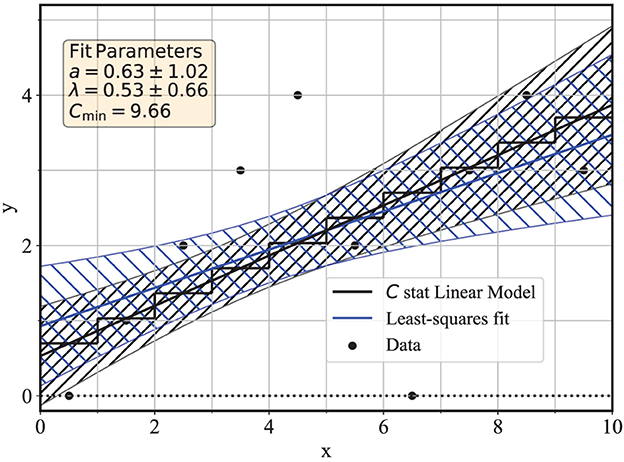
Figure 1. Linear regressions to days 0–9 of the COVID-19 data of Table 1. The black curves correspond to linear regression with the C statistics, and the blue curves for the ordinary least-squares regression.

The method of maximum-likelihood regression (see Section 2) makes use of two functions g(a) and F(a) that are reported in Figure 2. In this application, there is a total of M = 22 counts for N = 10 bins and n = 8 unique non-zero bins. According to (4), this results in n = 8 points of singularity for g(a) marked as green crosses in Figure 2, and n − 1 = 7 roots or zeros of g(a) marked as blue dots between consecutive singularities, with g′(a) < 0 in each interval. The roots of g(a) are also points of singularity for F(a), whose zero(s) are the estimates of the parameter a. Of the n − 2 = 6 solutions, only the last one is acceptable, i.e., it is the only value â that gives a non-negative model throughout its support, as required for Poisson counts (see Section 5 of [15]). Having identified the last singularity of F(a) as the last zero of g(a), the acceptable solution â is marked as the rightmost green dot in Figure 2.

FIGURE 2

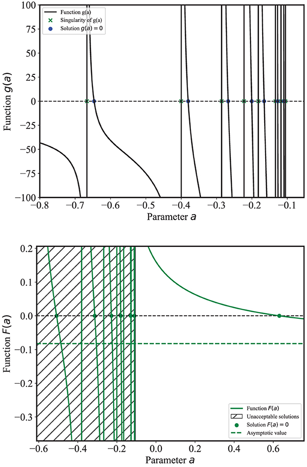
Figure 2. Functions g(a) and F(a) used for the Poisson regression, see Equation (4).

It is clear that it is not necessary to identify and calculate all the roots of g(a) in order to determine â but just the last one between the last two singularities of g(a). The computational burden is therefore very limited, even for data with a large number of events. Figure 2 report all points of singularities and the zeros for both g(a) and F(a) only for illustration purposes.

4.1.2. The covariance matrix

The error matrix evaluated according to (15) is

$\widehat{\epsilon }=\left[\begin{array}{cc}0.346& -0.665\\ -0.665& 1.044\end{array}\right]$

with the estimated standard deviations of the parameters also reported in the figure for estimated parameters â = 0.63 ± 1.02 and $\widehat{\lambda }=0.53\pm 0.66$.

4.1.3. The log-likelihood or C statistic

Moreover, the fit statistic is evaluated according to

$\begin{array}{ll}{C}_{\text{min}}={\displaystyle \sum _{i=1}^N}({\widehat{\mu }}_i-y_i+y_{i}ln\left(y_i/{\widehat{\mu }}_i\right)),& (21)\end{array}$

as reported in Equation 3 of [15]. Hypothesis testing with the C statistics requires the evaluation of critical values of its distribution, which is known only in the asymptotic limits of a large number of measurements N and for large parent means when C_min is approximately distributed as χ²(N − m) (see, e.g., [11, 33]), with m = 2 adjustable parameters. Although a detailed discussion of the method of hypothesis testing with the C statistics goes beyond the scope of this study, it is nonetheless useful to provide a brief description of its application for this example since hypothesis testing is an integral part of the overall regression. In the present example of small Poisson means, the approximation of C_min with a χ²(N − m) distribution is not accurate, and in [14], we proposed an approximate method to estimate critical values that applies also to the low-mean case. The method consists of using the parent mean and variance of each term in (21) in place of the mean and variance of a χ²(1) distribution (which are, respectively, 1 and 2) and use the central limit theorem to ensure an approximately normal distribution for the statistic. Following this method, the critical value of the C_min distribution for N − m = 8 degrees of freedom is 13.6 [compared to a corresponding critical value of 13.4 for the χ²(8) distribution], and therefore, these data are consistent with the null hypothesis of a linear model at the 90% confidence level. Notice how both the parameter estimation and the goodness-of-fit statistic naturally account for measurements with zero counts, such as bins 0 and 6.

4.1.4. The confidence band

The gray-hatched band associated with the best-fit model highlights another strength of the availability of the error matrix for the C statistic regression, which makes it is possible to estimate the variance of any function of the model parameters. In particular, it is often useful to estimate the variance of the expectation of the f_S(x) function for a fixed value of the independent variable x, i.e.,

${\widehat{f}}_S(x)=\text{E}[f_S(x)/x,\widehat{\theta }]=\widehat{\lambda }(1+â(1-x)),$

or, equivalently, for the expectation of the number of counts in a bin centered at x and with arbitrary bin size,

${ŷ}_x=\text{E}[y/x,\widehat{\theta }]=\widehat{\lambda }(1+â(1-x))\Delta x,$

where x is any value of the regressor variable, not limited to the values x_i that correspond to the measurements. The variance of the variable ŷ_x is represented by the variance of y values along a vertical line for a given x. The range ŷ_x±σ_yx is usually referred to as the confidence band of the best-fit model and is represented by the gray hatched region in Figure 1. The variance ${\sigma }_{y_x}^2$ is estimated by the error-propagation method, with

${\widehat{\sigma }}_{y_x}^2={\widehat{\sigma }}_{\lambda }^2{\left(\frac{\partial y_x}{\partial \lambda }\right)}^2{|}_{\widehat{\theta }}+{\widehat{\sigma }}_a^2{\left(\frac{\partial y_x}{\partial a}\right)}^2{|}_{\widehat{\theta }}+2{\widehat{\sigma }}_{\lambda a}^2\left(\frac{\partial y_x}{\partial \lambda }\right)\left(\frac{\partial y_x}{\partial a}\right){|}_{\widehat{\theta }}.$

The standard error σ_yx is therefore estimated immediately from the error matrix $\widehat{\epsilon }$ in (15) and from the analytical form for y_x. Similar condiderations can be extended to any function of the model parameters. Another useful application is to the overall slope of the model, which is measured as $â·\widehat{\lambda }=0.33\pm 0.15$ in this example.

4.2. Comparison to OLS regression

For comparison, Figure 1 also reports the ordinary least-squares fit to the same data, with uniform weights for all the points, with the linear model following the usual parameterization f(x) = a+bx. For completeness, a brief review of the OLS estimator is provided below.

4.2.1. OLS estimators

The OLS estimators are given by the usual formulas:

$\begin{array}{ll}{\widehat{\theta }}_{OLS}=\left[\begin{array}{c}â\\ \widehat{b}\end{array}\right]=\frac{1}{\Delta }\left[\begin{array}{c}{\displaystyle {\sum }_{i=1}^N}{x}_i^2·{\displaystyle {\sum }_{i=1}^N}{y}_i-{\displaystyle {\sum }_{i=1}^N}{x}_i·{\displaystyle {\sum }_{i=1}^N}{x}_i{y}_i\\ N{\displaystyle {\sum }_{i=1}^N}{x}_i{y}_i-{\displaystyle {\sum }_{i=1}^N}{x}_i·{\displaystyle {\sum }_{i=1}^N}{y}_i\end{array}\right]& (22)\end{array}$

with

$\Delta =N{\displaystyle \sum _{i=1}^N}{x}_i^2-{\left({\displaystyle \sum _{i=1}^N}{x}_i\right)}^2.$

The OLS regression is known to provide an unbiased estimate of the parameters, regardless of the parent distribution of the measurements, due to the linearity of the model (see, e.g., [9, 23]). As a result, Figure 1 shows that the C statistics and the OLS linear regressions provide qualitatively similar best-fit values.

4.2.2. Estimate of the covariance matrix for OLS

Under the assumption of a normal distribution with equal variance for all the measurements, the OLS method is equivalent to the maximum-likelihood method, and the value for the common variance is required to estimate the covariance matrix (e.g., see Chapter 11 of [11]). For measurements that are not normally distributed, such as the data model presented in this study and for this specific data example, it is still possible to provide an estimate of the parameter variances for the OLS estimators, if the OLS estimator are interpreted as a function of the measurements y_i, without requiring homoskedasticity or normality. In this case, the linear OLS is no longer a maximum-likelihood estimator, but it retains the convenient property of unbiasedness.

Using the assumption that y_i ~ Poisson(θ₀ + x_iθ₁) and that the measurements are independent, it follows that Var(y_i) = θ₀ + x_iθ₁, and therefore

$\begin{array}{ll}\text{Var}({\widehat{\theta }}_{OLS})\simeq \frac{1}{{\Delta }^2}\left[\begin{array}{c}{\displaystyle {\sum }_{i=1}^N}{\left({\displaystyle {\sum }_{i=1}^N}{x}_i^2-x_i{\displaystyle {\sum }_{i=1}^N}{x}_i\right)}^2·({\theta }_0+x_i{\theta }_1)\\ {\displaystyle {\sum }_{i=1}^N}{\left(N{x}_i-{\displaystyle {\sum }_{i=1}^N}{x}_i\right)}^2·({\theta }_0+x_i{\theta }_1)\end{array}\right]& (23)\end{array}$

Naturally, since the true parameters are unknown, one can only use these variances by substituting $\widehat{\theta }$ for θ in the right-hand side of (23). This simple result is due to the linearity of the model, and the independence of the measurements.

It is necessary to emphasize that the approximate variances derived in (23) are an ad-hoc estimate, and they do differ from the standard OLS error matrix⁴

$\begin{array}{ll}{\epsilon }_{OLS}=\frac{{\sigma }^2}{\Delta }\left[\begin{array}{cc}{\displaystyle {\sum }_{i=1}^N}{x}_i^2& -{\displaystyle {\sum }_{i=1}^N}{x}_i\\ \dots & N\\ \end{array}\right]& (24)\end{array}$

where σ² is the common (and unknown) variance. In the usual case of the OLS with equal variances, one would normally proceed with the estimation of σ² via the sum of square residuals, divided by N − k,

$\begin{array}{ll}{\widehat{\sigma }}^2=\frac{1}{N-k}{\displaystyle \sum _{i=1}^N}{(y_i-(â+\widehat{b}{x}_i))}^2& (25)\end{array}$

where k = 2 corresponds to the two adjustable parameters of the model. But such estimator would be biases for the case of heteroskedastic data and, therefore, not meaningful for this Poisson regression. This is the reason for the development of the ad-hoc approximation (23).

Moreover, an estimate for the covariance of the linear OLS estimators can be obtained by the usual error propagation method, namely,

${\widehat{\sigma }}_{ab}^2={\displaystyle \sum _{j=1}^N}\frac{\partial â}{\partial y_j}\frac{\partial \widehat{b}}{\partial y_j}{\sigma }_j^2,$

where ${\sigma }_j^2$ is the variance of the j-th measurement, in this application assumed to be Poisson-distributed. Notice that this method can also be used to obtain the error matrix (24) (e.g., see Section 11.3 of [11]). The result is

$\begin{array}{l}{\widehat{\sigma }}_{ab}^2=\frac{1}{{\Delta }^2}(\left(N{\displaystyle \sum _{i=1}^N{x}_i^2}+{\left({\displaystyle \sum _{i=1}^N{x}_i}\right)}^2\right){\displaystyle \sum _{j=1}^N{x}_j}{\sigma }_j^2\\ -{\displaystyle \sum _{i=1}^N{x}_i}\left({\displaystyle \sum _{i=1}^N{x}_i^2}{\displaystyle \sum _{j=1}^N{\sigma }_j^2}+N{\displaystyle \sum _{j=1}^N{x}_j^2}{\sigma }_j^2\right)),& (26)\end{array}$

which becomes the same as in (24) under the assumption of homoskedasticity. In (26), however, the variances to be used are the non-uniform Poisson-estimated ${\sigma }_j^2=â+x_j\widehat{b}$. In summary, it is still possible to estimate a covariance matrix for the linear OLS in place of the maximum-likelihood and Poisson-based (15). These estimates, (23) and (26), are obtained by a post facto use of the Poisson distribution in the usual OLS regression estimators, which in general do not require the specification of a parent distribution. The data of Figure 1 yield linear OLS parameters of a = 0.93 ± 0.80 and b = 0.25 ± 0.16 for a covariance ${\widehat{\sigma }}_{ab}^2=-0.11$, using (23) and (26). The confidence band according to these errors is reported as the blue hatched area in Figure 1.

For the purpose of comparison, the parameter uncertainties for the standard OLS regression according to (24) and (25) are also calculated. First, from the OLS best-fit parameters, Equation (25) yields an estimated common data variance of ${\widehat{\sigma }}^2=1.78$, and accordingly, the OLS error matrix yields errors that result in a = 0.93 ± 0.85 and b = 0.25 ± 0.15. In this application, the errors calculated for this “standard” OLS model is similar to those of the “modified” OLS model (a = 0.93 ± 0.80, b = 0.25 ± 0.16) and also to those with the “proper” Poisson regression of Section 4.1 (â = 0.63 ± 1.02 and $\widehat{\lambda }=0.53\pm 0.66$, with overall slope $â·\widehat{\lambda }=0.33\pm 0.15$). This chance agreement is in part the result of the fact that the Poisson data are consistent with the model, as determined by the analysis of the C statistics in Section 4.1.3. This agreement, however, is not guaranteed in every case, and the standard OLS regression for heteroskedastic data is not recommended (see, e.g., the discussion in Section 3.1 of the textbook by [9]).

Finally, it is worth noticing that a weighted least-squares (WLS) linear regression, with weights equal to the variances of the measurements⁵, is not recommended in this case. In fact, the WLS estimators depend on the unknown (and unequal) variances, and therefore, it is not possible to determine a priori a best-fit WLS model from which the Poisson variances for the error analysis is inferred, as was done in (23).

4.2.3. Goodness-of-fit analysis for OLS regression

Another difference between the maximum-likelihood C statistics regression and the OLS regression is with regard to goodness-of-fit testing. When the common variance is unavailable, as is generally the case for the OLS regression, the test statistics often used is

$\begin{array}{ll}t=\frac{\widehat{b}}{{\widehat{\sigma }}_b^2}~t(N-2),& (27)\end{array}$

where

$\begin{array}{ll}{\widehat{\sigma }}_b^2=\frac{(1-r^2)}{N-2}·\frac{{\displaystyle {\sum }_{i=1}^N}{(y_i-\overline{y})}^2}{{\displaystyle {\sum }_{i=1}^N}{(x_i-\overline{x})}^2}& (28)\end{array}$

is the sample variance of the slope b, and r is the linear correlation coefficient. Notice that this is a non-parametric estimate of the variance of the slope b, in that no assumptions on the distribution of the data are required. The linear correlation coefficient is defined by r² = bb′, where b is the usual slope of the linear regression of Y given X, and b′ is the slope of the linear regression of X given Y (see, e.g., Chapter 14 of [11]). This variance differs from that in (23), where the parent distribution of the measurement is used. From the observations that $a=\overline{y}-b\overline{x}$ and that $(1-r^2)\sum {(y_i-\overline{y})}^2/(N-2)$ is the non-parametric unbiased estimator of the sample variance of y, (28) yields a non-parametric estimate of the variance of the parameter a of the regression as

$\begin{array}{ll}{\widehat{\sigma }}_a^2={\widehat{\sigma }}_b^2\left(\frac{1}{N}{\displaystyle \sum _{i=1}^N}{(x_i-\overline{x})}^2+{\overline{x}}^2\right),& (29)\end{array}$

(see, e.g., Sections 11.5 and 14.3 of [11]).⁶ The test statistics (27) assumes that the parent slope is null (b = 0), and it is distributed like a Student's t distribution with N − 2 degrees of freedom, and it is sometimes referred to as the Wald statistics, after [35]. For these data, the linear correlation coefficient is r² = 0.273 for a value of t = 1.73, corresponding to a p-value of 0.12. Therefore, in the case of the OLS regression, the t-statistic provides an alternate non-parametric means to test the null hypothesis that the data are uncorrelated or with b = 0.

4.3. Fit to days 2–16 with a gap in the data, and non-uniform binning

In this example, the data for days 0 and 1 were ignored, the data for days 2–3 and 4–5 were combined into bins of size Δx = 2 days, the data for day 6 (where no events were reported) were ignored, and the datapoints for days 7–16 were kept with the original binning of Δx = 1 days, for a total of N = 12 measurements. These choices were simply made for illustration purposes. Specifically, it is generally not advisable to ignore a bin where no counts were recorded since the non-detection is actually positive information; a case with no counts-in-bin was provided in the previous example. Moreover the linear regression—and any non-linear regression as well—is sensitive to the choice of bin size. The choice of bin sizes must be dictated by an understanding of the data at hand and of the scientific goals of the regression.

4.3.1. Poisson regression

The results of the fit to these data are shown in Figure 3, for best-fit values of â = 0.31 ± 0.24, λ = 1.43 ± 0.85, and an error matrix of

$\widehat{\epsilon }=\left[\begin{array}{cc}0.716& -0.202\\ -0.202& 0.060\end{array}\right].$

It is illustrative to compare this estimate to the one from the error propagation method described in Section 3.4, which yields an estimated error matrix of

${\widehat{\epsilon }}_{ep}=\left[\begin{array}{cc}0.687& -0.200\\ -0.200& 0.061\end{array}\right],$

where the variance of the measurements y_k were approximated with the estimated parent means ${\widehat{\mu }}_k$. This covariance matrix is nearly identical to the one based on the information matrix, and the small differences between $\widehat{\epsilon }$ and ${\widehat{\epsilon }}_{ep}$ provide an example of the agreement between the two estimates. Figure 3 also shows the confidence band for the Poisson regression as the gray hatched area.

FIGURE 3

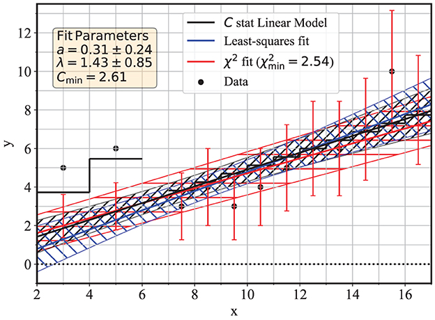
Figure 3. Linear regressions to days 2–17 of the COVID-19 data of Table 1, with a gap in the data, and non-uniform binning. The black curves correspond to linear regression with the Poisson-based C statistics, the blue curves corresponds to the ordinary least-squares regression, and the red curves corresponds to the χ² regression that assumes heteroskedastic errors reported as red error bars.

4.3.2. Comparison with OLS and χ² regression

For comparison, a maximum-likelihood regression using the χ² statistic was also performed for this example, and the results are shown as the red line and confidence band. The ordinary least-squares regression is also shown in blue. For the method of regression that minimizes the χ² statistic, the data are assumed to be normally-distributed, with variances equal to the number of counts in each bin. Given the variable bin size, the continuous lines, therefore, represent a density, i.e., the number of counts per unit interval of the x variable, which in this case it is time in units of days. This is reflected in the relationship between the function (1) in units of counts per unit y, and the parent mean in (2) in units of pure counts, which are related by the bin size Δx_i. Accordingly, in the χ² fit with non-uniform binning, the fit statistic is

${\chi }^2={\displaystyle \sum _{i=1}^N}{\left(\frac{y_i-{\mu }_i}{{\widehat{\sigma }}_i}\right)}^2$

where μ_i is given by (2) with a bin size Δx_i = 2 for i = 1, 2 and Δx_i = 1 for the other bins. Equivalently, the χ² regression can be performed directly to the function (1) (or to the linear model with the standard parameterization a+bx) by re-scaling both the measurements y_i and the errors ${\widehat{\sigma }}_i$ to counts per unit y since this is the usual assumption in standard software that is used for maximum-likelihood regression for normal data.⁷ Following this method, the first two data points have a count rate of one half of the values reported by the black dots, and the $\pm \widehat{\sigma }$ error bars for the χ² regression are illustrated as red vertical lines; those error bars have no meaning for the C statistic or the OLS regressions.

The overall slope of the C statistic regression line is aλ = 0.44 ± 0.11, while for the χ² regression it is 0.39 ± 0.13, and for the least-squares fit, it is 0.50 ± 0.08. The differences, albeit relatively small in this application, are the result of the different assumptions used in the modeling of the data, namely, the choice of Poisson vs. normal distribution for the number of counts in each bin.

5. Discussion and conclusion

This study has reviewed the [15] maximum-likelihood method of linear regression for Poisson count data and has presented an analytical method for the calculation of the covariance matrix for the parameters of a linear model. For this method of regression, it is found that the parameterization of the model of Equation 1, proposed by [20], is quite convenient due to its factorization of the two parameters, which results in convenient algebraic properties for the logarithm of the Poisson likelihood.

The method to obtain the covariance matrix is based on the Fisher information matrix, whose inverse approximates the covariance matrix in the asymptotic limit of a large number of measurement. The key result of this study is that it is possible to obtain a simple analytical expression for the covariance matrix (Equation 15) that can be used for the Poisson linear regression. This new result, together with the maximum-likelihood estimates of the parameters presented in [15], offers a simple and accurate method to perform linear regression on a variety of Poisson-distributed count data, including data with non-uniform binning and with the presence of gaps in the coverage of the independent variable. This method of regression for Poisson-distributed count data is, therefore, available for use in a variety of data applications, such as the one in the biomedical field presented in Section 4.

The study has also shown that an alternative method for the estimation of the covariance metrix, based on the error propagation or delta method, and also provides a simple analytical estimate that is in general good agreement with the method based on the information matrix. The main limitation in the use of the covariance matrix estimated from the information matrix (as well as that from the error propagation method) is that it applies only in the limit of a large number of measurements, where the maximum-likelihood estimates of the parameters are normally-distributed (e.g., [16, 25]). In this limit, the variance of the parameters and the covariance can be used for hypothesis testing assuming normal distribution of the parameters.

The maximum-likelihood linear regression to Poisson-distributed count data, presented in this study and in [15], have the advantages of being unbiased and asymptotically efficient, in the sense that, in the asymptotic limit of a large number of measurements, the estimators of the linear model parameters have the minimum variance bound according to the Cramér-Rao theorem ([24, 25], see also [34, 36]). Given that maximum-likelihood estimators are also known to be consistent in general (see, e.g., Chapter 18 of [34]), this method of regression has very desirable properties for the estimation of the linear model parameters. On the contrary, the ordinary least-squares regression does retain the convenient property of unbiasedness, even for the type of heteroskedastic variances that apply to these Poisson-distributed data. The OLS, however, is not guaranteed to be efficient, in the sense that the variances are in general larger than those of the maximum-likelihood method, and they can also be biased (e.g., [34, 37]). As a result, the OLS should be viewed as a less accurate method for the regression of Poisson-distributed count data.

Two other methods of linear regression also discussed in this study, the weighted least-squares and the χ² methods, suffer from more fundamental shortcomings when applied to integer-count Poisson data. In both cases, it is necessary to know a priori the unequal variances of the data, in order to proceed with the estimation, and this information is simply not available. In particular, the χ² method is often applied by making the assumption that the variances are equal to the square root of the counts, de facto assuming that the data are normally distributed and with variances equal to the measured counts. Although the Poisson distribution does converge to a normal distribution in the limit of a large number of counts (e.g., see Section 3 of [11]), the fact that the variance is approximated with the measured counts leads to a bias that remains even in the case of large-count data (e.g., [13, 14]). It is therefore not appropriate to use either of these two methods for the regression of Poisson-distributed count data.

Data availability statement

The original contributions presented in the study are included in the article/supplementary material, further inquiries can be directed to the corresponding author.

Author contributions

The author confirms being the sole contributor of this work and has approved it for publication.

Conflict of interest

The author declares that the research was conducted in the absence of any commercial or financial relationships that could be construed as a potential conflict of interest.

Publisher's note

All claims expressed in this article are solely those of the authors and do not necessarily represent those of their affiliated organizations, or those of the publisher, the editors and the reviewers. Any product that may be evaluated in this article, or claim that may be made by its manufacturer, is not guaranteed or endorsed by the publisher.

Footnotes

1. ^This modification is justified in Lemma 6.7 of [15].

2. ^The notation ∂²ln $\mathcal{L}$/∂θ∂θ′ indicates that diagonal elements are second derivatives with respect to the same parameter, and off-diagonal elements have cross-derivatives with respect to two different parameters. The symbol ^T indicates the transpose.

3. ^The New York Times archive reports the cumulative number of deaths, Table 1 also reports the daily counts.

4. ^See, e.g., Equation (11.19) of [11] or Example 19.6 of [34].

5. ^The weighted least-squares regression is discussed, for example, in heteroskedastic 19.17 of [34].

6. ^These formulas are implemented in the scipy.stats.linregress software.

7. ^For example, linregress or curve_fit in the scipy libraries. Such rescaling of units preserves the statistical properties of the measurements.

References

1. Poisson SD. Recherches sur la probabilit des jugements en mati re criminelle et en mati re civile. Paris (1837).

Google Scholar

2. Rutherford E, Chadwick J, Ellis C. Radiations from Radioactive Substances. Cambridge University Press (1920).

Google Scholar

3. Clarke RD. An application of the Poisson distribution. J Instit Act. (1946) 72:481.

Google Scholar

4. King G. Statistical models for political science event counts: bias in conventional procedures and evidence for the exponential Poisson regression model. Am J Polit Sci. (1988) 32:838–63.

Google Scholar

5. Campbell JE. Explaining presidential losses in midterm congressional elections. J Polit. (1985) 47:1140–57.

Google Scholar

6. Luria SE, Delbrück M. Mutations of bacteria from virus sensitivity to virus resistance. Genetics. (1943) 28:491–511.

PubMed Abstract | Google Scholar

7. Ross SM. Introduction to Probability Models. San Diego, CA: Academic Press (2003).

Google Scholar

8. Cash W. Parameter estimation in astronomy through application of the likelihood ratio. Astrophys. J. (1979) 228:939.

Google Scholar

9. Cameron C, Trivedi PK. Regression Analysis of Count Data. 2nd ed. Cambridge University Press (2013).

Google Scholar

10. Greenwood P, Nikulin M. A Guide to Chi-Squared Testing. Wiley (1996).

Google Scholar

11. Bonamente M. Statistics and Analysis of Scientific Data. 3rd ed. Singapore: Springer (2022).

Google Scholar

12. Lewis D, Burke CJ. The use and misuse of the chi-square test. Psychol Bull. (1949) 46:433–89.

Google Scholar

13. Kelly BC. Some aspects of measurement error in linear regression of astronomical data. Astrophys. J. (2007) 665:1489–506.

Google Scholar

14. Bonamente M. Distribution of the C statistic with applications to the sample mean of Poisson data. J Appl Stat. (2020) 47:2044–65. doi: 10.1080/02664763.2019.1704703

PubMed Abstract | CrossRef Full Text | Google Scholar

15. Bonamente M, Spence D. A semi–analytical solution to the maximum–likelihood fit of Poisson data to a linear model using the Cash statistic. J Appl Stat. (2022) 49:522–52. doi: 10.1080/02664763.2020.1820960

PubMed Abstract | CrossRef Full Text | Google Scholar

16. Fisher RA. On the mathematical foundations of theoretical statistics. Philos Trans R Soc Lond Ser A. (1922) 222:309–68.

Google Scholar

17. Hilbe JM. Modeling Count Data. Cambridge University Press (2014).

Google Scholar

18. Cameron AC, Trivedi PK. Econometric models based on count data. Comparisons and applications of some estimators and tests. J Appl Econometr. (1986) 1:29–53.

Google Scholar

19. McCullagh P, Nelder JA. Generalized Linear Models. 2nd ed. Chapman & Hall/CRC (1989).

Google Scholar

20. Scargle JD, Norris JP, Jackson B, Chiang J. Studies in astronomical time series analysis. VI. Bayesian block representations. Astrophys. J. (2013) 764:167. doi: 10.1088/0004-637X/764/2/167

CrossRef Full Text | Google Scholar

21. Ahoranta J, Nevalainen J, Wijers N, Finoguenov A, Bonamente M, Tempel E, et al. Hot WHIM counterparts of FUV O VI absorbers: evidence in the line-of-sight towards quasar 3C 273. Astronomy and Astrophysics. (2020) 634:A106. doi: 10.1051/0004-6361/201935846

CrossRef Full Text | Google Scholar

22. Levine AM, Bradt H, Cui W, Jernigan JG, Morgan EH, Remillard R, et al. First results from the all-sky monitor on the Rossi x-ray timing explorer. The Astrophysical Journal Letters. (1996) 469:L33.

Google Scholar

23. Eadie WT, Drijiard D, James M, Roos M, Sadoulet B. Statistical Methods in Experimental Physics. North Holland (1971).

Google Scholar

24. Rao CR. Information and accuracy attainable in the estimation of statistical parameters. Bull Calcutta Math Soc. (1945) 37:81.

Google Scholar

25. Cramer H. Mathematical Methods of Statistics. Princeton, NJ: Princeton University Press (1946).

Google Scholar

26. Amemiya T. Advanced Econometrics. Harvard University Press (1985).

Google Scholar

27. Shannon CE, Weaver W. The Mathematical Theory of Communication. Urbana, IL: University of Illinois Press (1949).

Google Scholar

28. Kullback S, Leibler RA. On information and sufficiency. Ann Math Stat. (1951) 22:79–86.

Google Scholar

29. Akaike H. A new look at the statistical model identification. IEEE Trans Automatic Control. (1974) 19:716–23.

Google Scholar

30. Fisher RA. Statistical Methods for Research Workers. Edinburgh: Oliver and Boyd (1925).

Google Scholar

31. Bevington PR, Robinson DK. Data Reduction and Error Analysis for the Physical Sciences. 3rd ed. McGraw Hill (2003).

Google Scholar

32. New York Times. GitHub (2021). Available online at: https://github.com/nytimes/covid-19-data/blob/master/us.csv

Google Scholar

33. Lampton M, Margon B, Bowyer S. Parameter estimation in X-ray astronomy. Astrophys. J. (1976) 208:177–90.

Google Scholar

34. Kendall M, Stuart A. The Advanced Theory of Statistics. Vol.2: Inference and Relationship. 3rd ed. New York, NY: Hafner (1973).

Google Scholar

35. Wald A. Tests of statistical hypotheses concerning several parameters when the number of observations is large. Trans Am Math Soc. (1943) 54:426–82.

Google Scholar

36. Rao CR. Linear Statistical Inference and Its Applications. 2nd ed. John Wiley and Sons (1973).

Google Scholar

37. Swindel BF. On the bias of some least-squares estimators of variance in a general linear model. Biometrika. (1968) 55:313–6.

Google Scholar