A statistical methodology for classifying earthquake detections and for earthquake parameter estimation in smartphone-based earthquake early warning systems

Smartphone-based earthquake early warning systems (EEWSs) are emerging as a complementary solution to classic EEWSs based on expensive scientific-grade instruments. Smartphone-based systems, however, are characterized by a highly dynamic network geometry and by noisy measurements. Thus, there is a need to control the probability of false alarms and the probability of missed detection. This study proposes a statistical methodology to address this challenge and to jointly estimate in near real-time earthquake parameters like epicenter and depth. The methodology is based on a parametric statistical model, on hypothesis testing and on Monte Carlo simulation. The methodology is tested using data obtained from the Earthquake Network (EQN), a citizen science initiative that implements a global smartphone-based EEWS. It is discovered that, when the probability to miss an earthquake is fixed at 1%, the probability of false alarm is 0.8%, proving that EQN is a robust smartphone-based EEW system.

1. Introduction

Wireless sensor networks (WSNs) enable solutions in multiple fields, and they are adopted in environmental, health, urban, and military applications [1, 2]. A problem commonly solved within WSNs is the detection and localization in space of relevant events or targets [3–7].

This study focuses on earthquake early warning systems (EEWSs) [8–10], which are deployed in seismic areas for the real-time detection of earthquakes, with the ultimate goal of sending alerts to citizens and stopping critical processes before ground shaking begins.

Classic EEWSs are based on a dense network of scientific-grade instruments, with construction and operating costs on the order of millions of euros [11]. This largely limited their implementation, especially in seismic developing countries.

Due to smartphone technology, low-cost EEWSs have been recently implemented at the global level [12]. Smartphones are used to detect ground shaking using the on-board accelerometer, and a warning is issued to the population as soon as the earthquake is detected. This path has been explored by the Earthquake Network (EQN), a citizen science initiative [13, 14], that, since 2013, implements the first smartphone-based EEWS.

Within the EQN EEWS, nodes of the WSN are the smartphones voluntarily made available by citizens. This poses many challenges because personal smartphones mainly sense the “anthropic noise” connected with human activities.

The primary challenge faced by the EQN is to control the probability of false alarms and the probability to miss an earthquake. Alerts may be triggered by events unrelated to earthquakes and some (possibly strong) earthquakes may be missed, especially if the number of monitoring smartphones is small. Both false alarms and missed detections may undermine people's trust in the EQN.

In the pivotal study by Finazzi and Fassò [15], a statistical methodology is developed for identifying in real-time earthquake occurrence. The study, however, does not take into account the spatial dimension of the smartphone network, making the detection algorithm prone to false alarms. Moreover, the methodology does not allow to estimate important earthquake parameters such as epicenter and depth. In Finazzi et al. [16], instead, the EQN detection capabilities are modeled within a probabilistic framework. It is discovered that the EQN missed some relatively strong earthquakes that were supposed to be detected by the smartphone network. These considerations and findings suggest that there is room to improve EQN's methods and algorithms.

This study proposes a statistical methodology for 1) controlling the probability of false alarms, 2) controlling the probability of missed detection, 3) classifying a detection between true and false earthquake, and 4) estimating earthquake epicenter and depth (if the detection is classified as a true earthquake).

The methodology is based on a statistical parametric model, statistical hypothesis testing, and Monte Carlo simulation. Contrary to model-less approaches (see for instance [3]), the methodology exploits the fact that the spatio-temporal dynamic of seismic waves is well-known. This information is retained by the statistical model, and it helps to both classify the EQN detection and to estimate the earthquake parameters.

Due to the peculiarity of the specific application, real-time is a constraint. Ideally, classification and earthquake parameter estimation should not exceed 1 or 2 s of computing time.

The smartphone-based EQN is used to test the statistical methodology, which is then applied to some true and false EQN detections.

2. EQN's detection algorithm

Before formalizing the classification and the earthquake parameter estimation problems, it is useful to detail the output of the earthquake detection algorithm currently implemented by the EQN [15]. For any given area of radius 30 km, the algorithm compares the number of triggering smartphones in the last 10 s with the number of active smartphones. A triggering smartphone is a smartphone that detected an acceleration above a threshold, while an active smartphone is a smartphone known to monitor earthquakes. If the ratio between triggering smartphones and active smartphones exceeds a threshold, an earthquake is claimed to be detected. The output of the detection algorithm consists of the detection location and the list of the triggering smartphones (triggers for short), which are identified by their spatial coordinates (latitude and longitude) and the triggering time.

3. Problem formalization

An earthquake detection made by an EQN is defined in terms of k_j>0 triggers, where j is the index of the generic detection. In general, k_j is not a constant, meaning that each detection is characterized by a different number of triggers. Each trigger is described by the feature vector as follows:

$\begin{array}{l}{\text{x}}_i=(t_i,la{t}_i,lo{n}_i),i=1,...,k_j,\end{array}$

where t_i∈ℝ is the triggering time, while $(la{t}_i,lo{n}_i)\in {{S}}^2$ are the smartphone coordinates, with ${{S}}^2$ being the sphere embedded in ℝ³. The k_j×3 matrix $\text{X}={\left({\text{X}}_1^{\prime },...,{\text{X}}_{k_j}^{\prime }\right)}^{\prime }$ is the data point, and the feature space is ${X}={\cup }_{k=1}^{\infty }{{X}}_k$, with ${{X}}_k={ℝ}^k\times {({{S}}^2)}^k$ and k > 0 is the generic number of triggers.

Let ${Y}=\left\{-1,1\right\}\ni y$ be the label space. For each earthquake detection, y = 1 if the detection is false while y = −1 if the detection is related to a true earthquake.

The aim is to learn a hypothesis map $h:{X}\to {Y}$ such that y≈h(X) for any data point X (i.e., for any future EQN detection). The map h is highly non-linear since the information content of X is determined by the spatio-temporal dynamics of the seismic waves and spatial distribution of the smartphones at the time of the earthquake.

A statistical parametric model $f:{X}\to \Theta$ is adopted to understand if X is generated by a true earthquake. The unknown model parameter vector is θ∈Θ = ℝ^s, with s≪k_j as the vector size. The hypothesis map is then h(X) = g(f(X)) = g(θ). Note that s is constant, and it does not depend on the dimension of X.

When dealing with EEW systems, it is required to control two parameters: the probability α of missed detections (true earthquakes which are not detected by the system) and the probability β of false detections (detections which are not related to any occurred earthquake). It is thus reasonable to adopt a 0/1 loss function as follows:

$L\left(\left(\text{X},y\right),g\right)=\{\begin{array}{l}1\text{ if }y\ne \widehat{y}\\ 0\text{ else,}\end{array}$

and to learn a g that minimized the Bayes risk

$\begin{array}{ll}ĝ={\displaystyle \underset{g}{arg min}}E(L((\text{X},y),g)).& (1)\end{array}$

As discussed by Jung [17], solving (Equation 1) requires knowing the joint probability distribution p(X, y). Instead, we rely on the fact that it is relatively easy to simulate EQN detections under different smartphone geometries and different earthquake parameters. This induces a variability on X and on the number of triggers k_j. Assuming to have a data set ${D}=({\text{X}}^{(1)},y^{(1)}),...,({\text{X}}^{(m)},y^{(m)})$ and that ${D}$ is a representative sample of p(X, y), we define the empirical risk as follows:

$\begin{array}{l}L(g\mid {D})=(1/m){\displaystyle \sum _{j=1}^m}L(({\text{X}}^{(j)},y^{(j)}),g),\end{array}$

and g is learned from the following minimization problem:

$\begin{array}{ll}ĝ={\displaystyle \underset{g}{arg min}}L(g\mid {D}).& (2)\end{array}$

Note that solving (Equation 2) is equivalent to solve

$\begin{array}{ll}ĝ={\displaystyle \underset{g}{arg min}}\alpha (g)+\beta (g),& (3)\end{array}$

where it is made explicit that the probabilities of missed and false detections depend on g.

From an EEW perspective, the solution provided by Equation (3) is not necessarily the best. In some contexts, a missed detection has a larger negative impact than a false detection, while in other contexts, it is the opposite. In this case, one probability is fixed to the desired level, and the other probability is minimized. Two other minimization problems for learning g are the following:

$\begin{array}{ll}ĝ={\displaystyle \underset{g}{arg min}}\alpha (g)+\beta ,& (4)\end{array}$

$\begin{array}{ll}ĝ={\displaystyle \underset{g}{arg min}}\alpha +\beta (g).& (5)\end{array}$

4. Statistical parametric model and classification

In this section, we propose a statistical parametric model for the generic data point X. The observed triggering time for a smartphone sensing an earthquake is modeled as

$\begin{array}{ll}{t}_i=t_i^{*}+{ϵ}_i,i=1,...,k_j,& (6)\end{array}$

where $t_i^{*}$ is the expected triggering time, while ${ϵ}_i~N(0,{\sigma }_{ϵ}^2)$ is a random component. More in detail

$\begin{array}{ll}{t}_i^{*}=\frac{D_{i,H}}{v}+t_O,& (7)\end{array}$

with

$\begin{array}{ll}{D}_{i,H}=\sqrt{d_E^2+4R(R-d_E)sin{\left(\frac{D_{i,E}}{2R}\right)}^2},& (8)\end{array}$

as the distance between the hypocentre and the smartphone location, v is the seismic wave speed, and t_O∈ℝ is the earthquake origin time.

In Equation (8), D_{i, E} is the distance between the epicenter $(la{t}_E,lo{n}_E)\in {{S}}^2$ and the smartphone location, d_E∈[0, 500] is the earthquake depth, and R is the earth radius (6, 371 km). Here, it is assumed that all smartphones either detect the primary seismic wave (v = 7.8 km/s) or they all detect the secondary wave (v = 4.5 km/s). This assumption is justified by the fact that earthquake detection is based on smartphones within a radius of 30 km, which is a relatively small area.

The role of the random component ϵ_i is to model the difference between the expected and the observed triggering time. This difference is mainly due to the smartphone detection delay and a seismic wave velocity that may differ from the expected value.

Equations (6–8) fully define the statistical model f and the model parameter vector is $\theta =(la{t}_E,lo{n}_E,d_E,t_O,{\sigma }_{ϵ}^2)\in \Theta ={{S}}^2\times \left[0,500\right]\times ℝ\times {ℝ}^{+}\subset {ℝ}^6$.

4.1. Model estimation

Model estimation is based on the maximum likelihood method. For a generic EQN detection, the log-likelihood function based on the joint probability distribution of $\Delta t_i=t_i-t_i^{*}$ is

$\begin{array}{ll}l(\theta ;\text{X})=-\frac{k}{2}ln2\pi -\frac{k}{2}ln{\sigma }_{ϵ}^2-\frac{1}{2{\sigma }_{ϵ}^2}{\displaystyle \sum _{i=1}^k}\Delta t_i^2.& (9)\end{array}$

The Δt_i are assumed to be independent. This assumption is realistic because smartphones do not share a common clock, detection delays are independent, and the detection by each smartphone is influenced by local factors (e.g., where the smartphone is located, at which floor of the building, and the accelerometer sensitivity).

Maximum likelihood estimates of lat_E, lon_E, d_E, and t_O are given by

$\begin{array}{ll}{\displaystyle \underset{la{t}_E,lo{n}_E,d_E,t_O}{arg min}}{\displaystyle \sum _{i=1}^k}\Delta t_i^2.& (10)\end{array}$

The solution of Equation (10) cannot be obtained in a closed form due to the non-linearity of Equation (8) hence, estimates are obtained via numerical optimization using the BFGS Quasi-Newton method [18]. As usual, to avoid local minima, the numerical optimization algorithm is run multiple times starting from random initial values for lat_E, lon_E, d_E, and t_O. The minimization in Equation (10) is possible because for any “proposed” values of the model parameters, $t_i^{*}$ can be computed using Equations (7), (8) and then compared with the observed t_i.

At convergence, the BFGS quasi-network method also returns the Hessian matrix. Since maximum likelihood estimates for model parameters are obtained from a minimization problem, the Hessian is equivalent to the observed Fisher information matrix. The variance–covariance matrix of the three parameters is then the inverse of the Hessian matrix from which standard errors are easily computed.

Finally, the maximum likelihood estimate of the variance is as follows:

$\begin{array}{ll}{\widehat{\sigma }}_{ϵ}^2=\frac{1}{k}{\displaystyle \sum _{i=1}^k}{(\widehat{\Delta t_i}-\widehat{\mu })}^2,& (11)\end{array}$

where $\widehat{\Delta t_i}=t_i-{\widehat{t}}_i^{*}$ is computed after replacing in Equations (7) and in Equation (8) the maximum likelihood estimates of latitude, longitude, and depth, while $\widehat{\mu }$ is the mean of the $\widehat{\Delta t_i}$.

4.2. EQN detection classification

Among all elements of θ, the parameter that carries information about how the EQN detection should be classified is ${\sigma }_{ϵ}^2$. Indeed, ${\widehat{\sigma }}_{ϵ}^2$ tends to be small when the earthquake is true (and triggering times follow the seismic wave dynamic) while ${\widehat{\sigma }}_{ϵ}^2$ tends to be large when the detection is not related to an earthquake event. This implies that g(θ) reduces to $g({\sigma }_{ϵ}^2)$.

In this study, g is chosen to be a statistical hypothesis test on ${\sigma }_{ϵ}^2$. The system of hypothesis is given by

$\begin{array}{ll}\{\begin{array}{c}{H}_0:{\sigma }_{ϵ}^2=\delta \\ H_1:{\sigma }_{ϵ}^2>\delta .\end{array}& (12)\end{array}$

The null hypothesis is rejected when the variance is higher than expected, namely, when smartphone triggering times do not follow the propagation law of the primary or secondary seismic wave. As customary in the statistical hypothesis testing, the probability α is fixed, and it represents the probability to reject the null hypothesis when it is actually true (namely, it is the probability to miss a true earthquake).

The test statistic is as follows:

$\begin{array}{ll}T=df\frac{{{\sigma }_{ϵ}}^2}{\delta },& (13)\end{array}$

which, under the null hypothesis, is distributed as a chi-square with k−4 degrees of freedom (df), where 4 is the number of estimated parameters in Equation (10). The null hypothesis is rejected if $\widehat{T}>q_{(1-\alpha ),df}$, where $\widehat{T}$ is obtained replacing ${\sigma }_{ϵ}^2$ with ${\widehat{\sigma }}_{ϵ}^2$ in Equation (13), while q_{(1−α), df} is the (1−α)-quantile of a chi-square distribution with df degrees of freedom, usually called the critical value. In practice, an EQN detection is a true earthquake unless data bring enough evidence that the detection is actually false.

Since we do not know which seismic wave is detected by the smartphones, two models f are estimated: one with v = 7.8 km/s and another with v = 4.5 km/s in Equation (7). This brings to two estimated values for ${\sigma }_{ϵ}^2$ and two hypothesis tests are implemented. The detection is classified as a false earthquake if the null hypothesis is rejected under both tests; otherwise, the earthquake is classified as true.

It is worth noting that the statistical hypothesis test is equivalent to a linear map. Indeed, setting

$\begin{array}{ll}w={\left(\frac{1}{\delta },1\right)}^{\prime },& (14)\end{array}$

$\begin{array}{ll}\varphi ={\left(df{\widehat{{\sigma }_{ϵ}}}^2,-q_{(1-\alpha ),df}\right)}^{\prime },& (15)\end{array}$

then g = w′ϕ, and the earthquake detection classification is based on the following rule:

$\begin{array}{ll}\widehat{y}=\{\begin{array}{l}-1\text{ if }{w}^{\prime }\varphi <0\\ 1\text{ else}.\end{array}& (16)\end{array}$

Finally, δ is obtained by solving the problem

$\begin{array}{ll}\widehat{\delta }={\displaystyle \underset{\delta }{arg min}}\alpha +\beta (\delta ).& (17)\end{array}$

Algorithm 1 summarizes the steps for classifying an EQN detection and for estimating the earthquake parameters in case the detection is classified as a true earthquake.

ALGORITHM 1

Algorithm 1. EQN detection classification and earthquake parameters estimation.

5. Simulation study

The minimization problem in Equation (17) has no closed-form solution. For this reason, we implement a Monte Carlo simulation that aims to simulate a data set ${D}$ and to minimize Equation (17).

A total of 1,000 true EQN detections and 1,000 false EQN detections are simulated considering the true locations of 1,000 smartphones of the EQN in Lima (Peru).

The probability of missed detection is fixed to α = 0.01 while δ is made varying from 0.1 to 1.5 with step 0.1. For each value of δ, β(δ) is computed by estimating the model f and by implementing the hypothesis test (Equation 13) overall data points X^(j) in ${D}$. Finally, $\widehat{\delta }$ is the value of δ that minimizes β(δ).

5.1. Simulation of true detections

For simulating a true earthquake, the following aspects are taken into account: the earthquake epicenter and depth, the arrival time of the seismic wave at the smartphone locations, the earthquake detectability by the smartphone, and the error on the triggering time. Finally, we account for the fact that smartphones may detect events unrelated to the earthquake.

The epicenter locations (lon_E and lat_E) are simulated uniformly inside the coordinates box [−12.39°, −11.74°] for latitude and [−77.17°, −76.66°] for longitude. The box encompasses the EQN of Lima. On the contrary, the earthquake depth is simulated uniformly in the range [0, 100] km independently of the earthquake epicenter.

The arrival time of the seismic wave at each smartphone location is simulated from Equation (6) assuming t_O = 0 and v = 7.8 km/s. Only 70% of smartphones are made triggering because of the earthquake. For these smartphones, the error on the triggering time is simulated from a zero mean normal distribution with variance ${\sigma }_{\epsilon }^2=1.67$. Such variance guarantees that the 1st and the 99th percentiles of the error distribution are around −3 and 3 s, respectively, which are realistic values for an error on the triggering time.

Of the remaining 30% of smartphones which do not trigger, 6% are made triggering at random with a triggering time uniformly generated in the range [0, 12] s. This implies that when the earthquake is detected by the EQN detection algorithm, the list of triggering smartphones may include triggers unrelated to the earthquake dynamic.

Once the list of triggering smartphones is defined and sorted by triggering time, the EQN detection algorithm is applied to the list. The algorithm stops when the detection condition is satisfied, and the sub-list of triggers that concurred with the earthquake detection is given as the output.

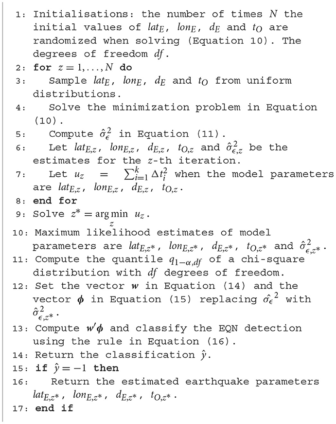
Figure 1 shows an example of a simulated true earthquake. Two separated regions can be visually identified, one with triggering smartphones (those that concurred with the detection) and another with non-triggering smartphones not yet reached by the seismic waves.

FIGURE 1

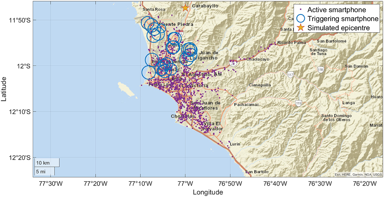
Figure 1. Simulated true earthquake detection based on the EQN smartphone network of Lima (Peru). The diameter of circles is proportional to the triggering time.

5.2. Simulation of false detections

To simulate a false detection, we assume that smartphones trigger at random with a triggering time that does not follow the law of seismic wave propagation. Only 30% of the smartphones are made triggering, and the triggering time is uniformly sampled in the range [0, 12] s.

Figure 2 shows an example of a simulated false EQN detection. Contrary to true earthquakes, no specific spatial pattern on the triggers is observed.

FIGURE 2

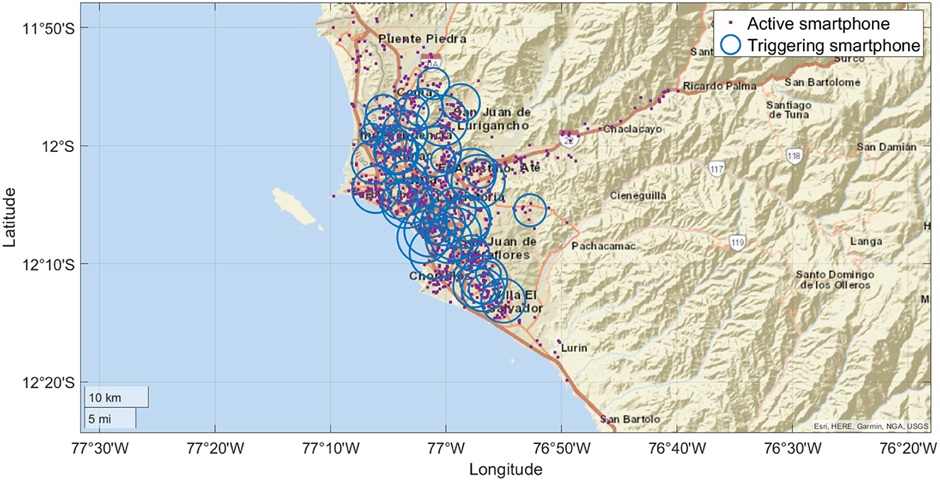
Figure 2. Simulated false earthquake detection based on the EQN smartphone network of Lima (Peru). The diameter of circles is proportional to the triggering time.

5.3. Simulation results

The minimization of Equation (17) is attained when $\widehat{\delta }=0.6$ and β is found to be equal to 0.008 (conditionally on α = 0.01). Figure 3 shows the empirical distributions of ${\widehat{\sigma }}_{ϵ}^2$ for both true and false simulated EQN detections. Although the detection classification is based on the hypothesis test (and not directly on ${\widehat{\sigma }}_{ϵ}^2$), the overlapping between distributions suggests that classification errors are possible.

FIGURE 3

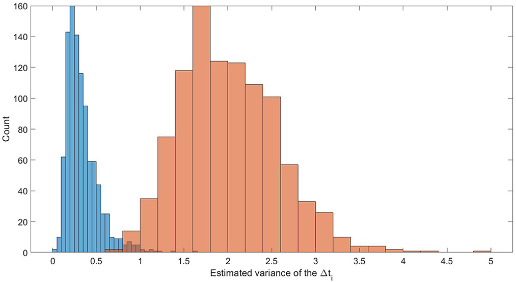
Figure 3. Empirical distributions of ${\widehat{\sigma }}_{ϵ}^2$ under simulated true detections (blue histogram) and under simulated false detections (red histogram).

A by-product of detection classification is the estimate of the earthquake parameters. Figure 4 shows the box plots of errors on earthquake epicenter and depth. Both errors have a median of around 18 km, suggesting that along with the detection classification (true/false), the model output can be exploited to provide preliminary estimates of the earthquake parameters.

FIGURE 4

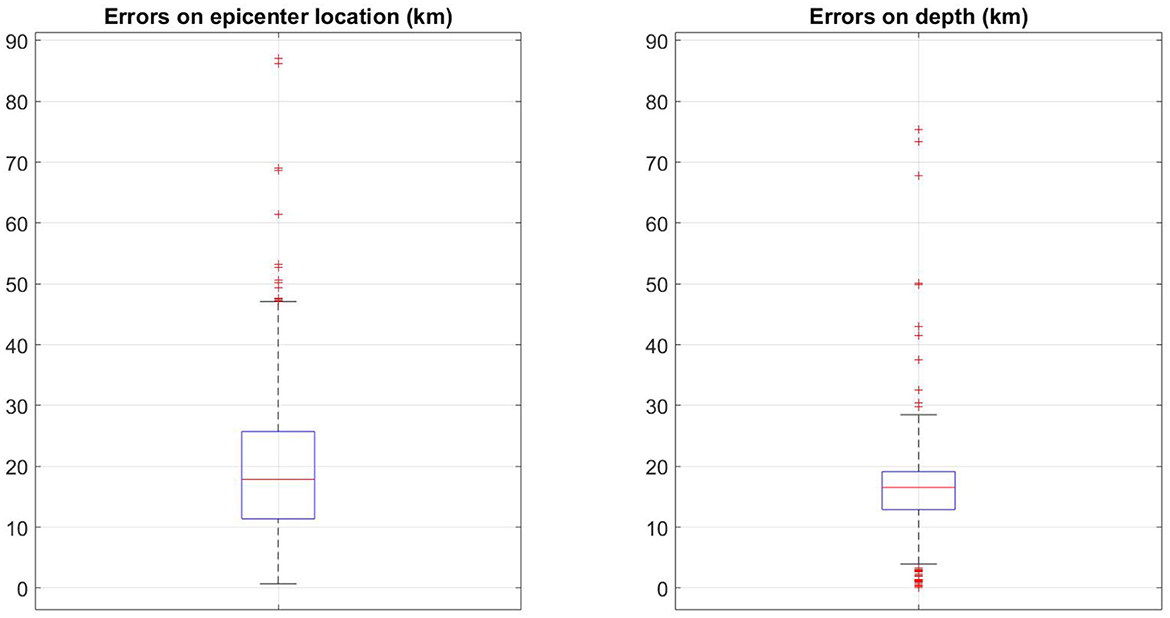
Figure 4. Box plot of the errors on epicenter location (lat_E, lon_E) (left) and box plot of the errors on earthquake depth d_E (right) for the 1,000 simulated true earthquake detections.

6. Real data example

The methodology developed in this study is applied to true and false detections made by the EQN. As a true earthquake, the event occurred near Genova (Italy) on 4 October 2022 at 21:41:10.5 UTC is considered. Figure 5 depicts the triggering smartphones (n = 21), while estimation and classification results are reported in Table 1 for v = 7.8 and v = 4.5 km/s, respectively.

FIGURE 5

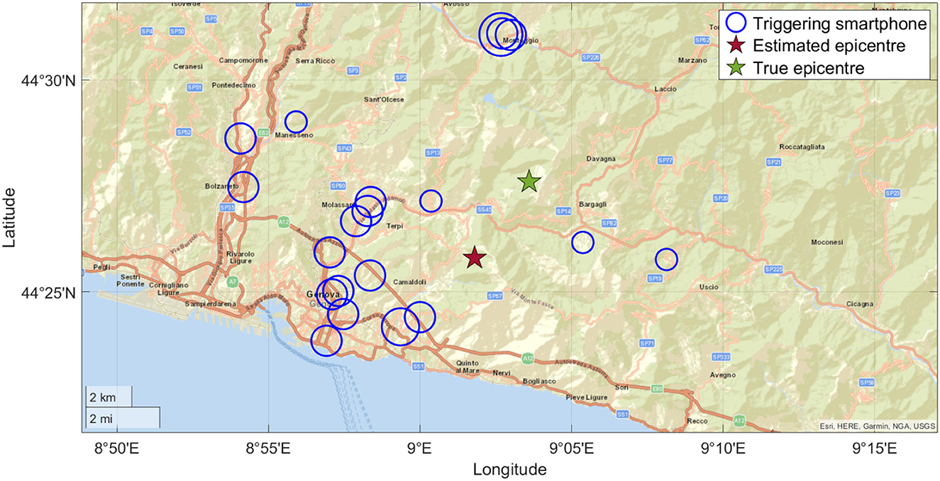
Figure 5. EQN triggers for the earthquake occurred on 4 October 2022 close to Genoa (Italy). The diameter of circles is proportional to the triggering time.

TABLE 1

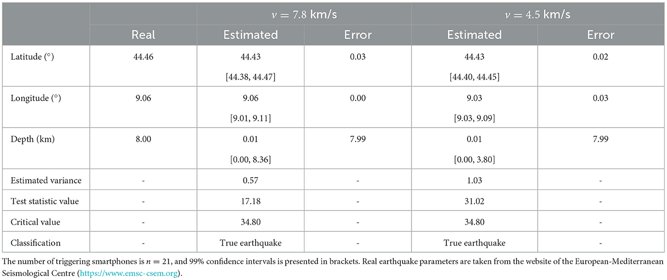
Table 1. Detection classification and earthquake parameters estimation for the EQN detection near Genova (Italy) assuming v equal to 7.8 and 4.5 km/s.

For both seismic wave velocities, we can observe that latitude and longitude are accurately estimated, while the error in depth is not negligible. Nonetheless, the true values are within the 99% confidence intervals evaluated from the standard errors on the model parameters. In addition, the earthquake is classified as true under both velocities since both observed test statistics are lower than the test critical value. This happens because triggers are close to the epicenter, and primary and secondary seismic waves are nearly concurrent.

The estimation and classification results were obtained in less than 1 s using an Intel(R) Core(TM) i7-9750H CPU @2.60GHz, suggesting that the approach can be adopted for real-time applications.

Figure 6 shows the n = 108 triggers of a false detection occurred near Acapulco (Mexico) on 25 September 2022, at 09:55:45 UTC. In this case, the computed test statistics are 1039.7 and 1026.0 for v = 4.5 and 7.8 km/s, respectively, while the critical value is 141.62. H₀ is rejected in both cases and the detection is claimed as false. In this particular case, the detection was caused by a strong lightning bolt. The speed of sound, however, is around 0.3 km/s, a value much smaller than the speed of primary and secondary seismic waves.

FIGURE 6

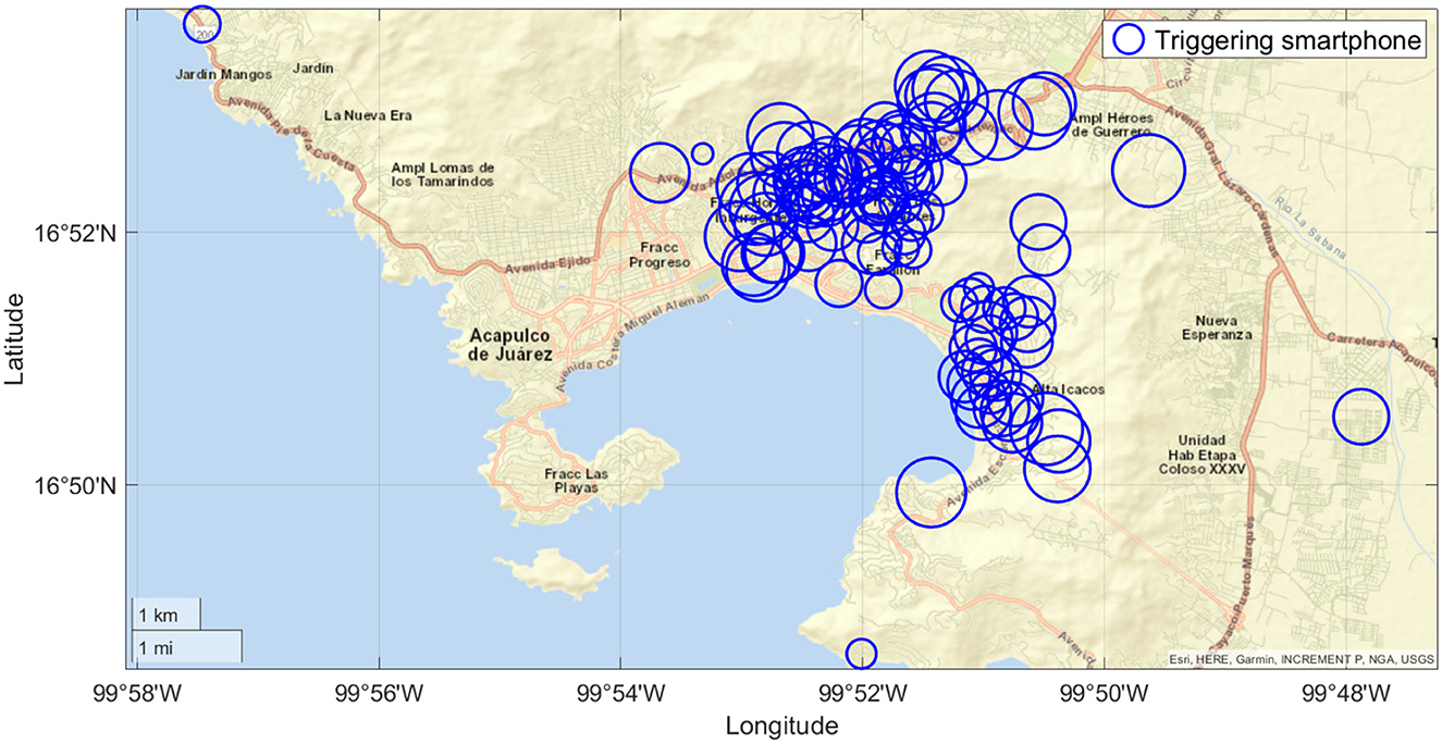
Figure 6. Triggers for the false EQN detection occurred on 25 September 2022, close to Acapulco (Mexico). The diameter of circles is proportional to the triggering time.

7. Discussion

The methodology developed in this study allows to classify detections made by smartphone-based earthquake early warning systems between true (related to a real earthquake) and false. This is done analyzing the information content of the smartphone triggers that contributed to the detection.

With respect to classic classification problems, the data point describing the triggers has a varying dimension which depends on the smartphone network geometry. The proposed solution is based on two steps. First, a statistical parametric model is used to convert the data point into a parameter vector with a fixed (and small) dimension. Second, a hypothesis test is implemented for classification.

While we do not claim our choices of f and g to be optimal, both steps are based on well-established statistical methods. With respect to the specific choice of g, it is worth discussing that a simpler alternative is the linear map g^* = δ′ϕ, with δ = (δ, 1)′ and $\varphi ={(1,-{\widehat{\sigma }}_{ϵ}^2)}^{\prime }$. In this case, the classification is based on the more intuitive comparison ${\widehat{\sigma }}_{ϵ}^2⋛\delta$. This simpler solution, however, does not take into account neither the actual number of triggers for the specific detection (10 or 1,000 makes a difference in the uncertainty of ${\widehat{\sigma }}_{ϵ}^2$) nor the fact that the distribution of ${\sigma }_{ϵ}^2$ is known under the null hypothesis (that the detection is related to a true earthquake). Using hypothesis testing, we are thus able to retain a part of the information which is lost when X is synthesized with θ.

8. Conclusion

Classification and earthquake parameter estimation are performed in near real time, making the statistical methodology suitable to be implemented in operational systems. On the contrary, the methodology does not fully exploit the information available on the EQN system. Specifically, the modeling is only on the triggering smartphones, while the active non-triggering smartphones are ignored. Knowing, at the EQN detection time, which smartphones have not (yet) triggered may better constraint epicenter and depth, thus improving their estimates.

In addition, for an EEWS like EQN that works globally, it would be important to study if the data set ${D}$ generated by the Monte Carlo simulation is a representative sample of p(X, y). If not, the observed α and β probabilities might deviate from the expected ones.

Finally, a limit of the approach proposed by this study is that the statistical methodology is applied downstream of EQN detections. Ideally, the detection, the classification, and the earthquake parameter estimation problems should be jointly addressed in a unified approach. In this regard, the vast literature on wireless sensor networks may help propose a solution under the real-time constraint.

These open problems, along with the estimation of the earthquake magnitude, will be the focus of future works.

Data availability statement

The raw data supporting the conclusions of this article will be made available by the authors, without undue reservation.

Author contributions

FF: conceptualization, writing–review, and editing. FM: investigation, methodology, validation, and writing–original draft preparation. All authors contributed to the article and approved the submitted version.

Funding

This article was funded by the European Union's Horizon 2020 Research and Innovation Program under grant agreement RISE No. 821115.

Acknowledgments

Authors thank the reviewers and the associate editor for the well-targeted suggestions that considerably improved the quality of the article.

Conflict of interest

The authors declare that the research was conducted in the absence of any commercial or financial relationships that could be construed as a potential conflict of interest.

Publisher's note

All claims expressed in this article are solely those of the authors and do not necessarily represent those of their affiliated organizations, or those of the publisher, the editors and the reviewers. Any product that may be evaluated in this article, or claim that may be made by its manufacturer, is not guaranteed or endorsed by the publisher.

Author disclaimer

Opinions expressed in this article solely reflect the authors' views and the EU is not responsible for any use that may be made of information it contains.

References

1. Elson J, Estrin D. Sensor networks: a bridge to the physical world. In: Wireless Sensor Networks. Boston, MA: Springer (2004). p. 3–20.

Google Scholar

2. Arampatzis T, Lygeros J, Manesis S. A survey of applications of wireless sensors and wireless sensor networks. In: Proceedings of the 2005 IEEE International Symposium on, Mediterrean Conference on Control and Automation Intelligent Control. Limassol: IEEE (2005). p. 719–24.

Google Scholar

3. Katenka N, Levina E, Michailidis G. Local vote decision fusion for target detection in wireless sensor networks. IEEE Trans Signal Process. (2007) 56:329–38. doi: 10.1109/TSP.2007.900165

CrossRef Full Text | Google Scholar

4. Huang C, Hsing T, Cressie N, Ganguly AR, Protopopescu VA, Rao NS. Bayesian source detection and parameter estimation of a plume model based on sensor network measurements. Appl Stochastic Models Business Ind. (2010) 26:331–48. doi: 10.1002/asmb.859

CrossRef Full Text | Google Scholar

5. Khadivi A, Hasler M. Fire detection and localization using wireless sensor networks. In: Sensor Applications, Experimentation, and Logistics: First International Conference, SENSAPPEAL 2009 Athens, Greece, September 25. 2009 Revised Selected Papers 1. Athens: Springer (2010). p. 16–26.

PubMed Abstract | Google Scholar

6. Hazart A, Giovannelli JF, Dubost S, Chatellier L. Inverse transport problem of estimating point-like source using a Bayesian parametric method with MCMC. Signal Process. (2014) 96:346–61. doi: 10.1016/j.sigpro.2013.08.013

CrossRef Full Text | Google Scholar

7. Ciuonzo D, Rossi PS. Distributed detection of a non-cooperative target via generalized locally-optimum approaches. Inf Fusion. (2017) 36:261–74. doi: 10.1016/j.inffus.2016.12.006

CrossRef Full Text | Google Scholar

8. Gasparini P, Manfredi G, Zschau J. Earthquake Early Warning Systems. Berlin: Springer (2007).

Google Scholar

9. Satriano C, Wu YM, Zollo A, Kanamori H. Earthquake early warning: concepts, methods and physical grounds. Soil Dyn Earthquake Eng. (2011) 31:106–18. doi: 10.1016/j.soildyn.2010.07.007

CrossRef Full Text | Google Scholar

10. Cremen G, Galasso C. Earthquake early warning: recent advances and perspectives. Earth Sci Rev. (2020) 205:103184. doi: 10.1016/j.earscirev.2020.103184

CrossRef Full Text | Google Scholar

11. Given DD, Cochran ES, Heaton T, Hauksson E, Allen R, Hellweg P, et al. Technical Implementation plan for the ShakeAlert Production System: An Earthquake Early Warning System for the West Coast of the United States. Reston, VA: U.S. Department of the Interior, US Geological Survey (2014).

Google Scholar

12. Finazzi F. The earthquake network project: toward a crowdsourced smartphone-based earthquake early warning system. Bull Seismol Soc Am. (2016) 106:1088–99. doi: 10.1785/0120150354

CrossRef Full Text | Google Scholar

13. Finazzi F. The earthquake network project: a platform for earthquake early warning, rapid impact assessment, and search and rescue. Front Earth Sci. (2020) 8:243. doi: 10.3389/feart.2020.00243

CrossRef Full Text | Google Scholar

14. Bossu R, Finazzi F, Steed R, Fallou L, Bondár I. “Shaking in 5 Seconds!”–performance and user appreciation assessment of the earthquake network smartphone-based public earthquake early warning system. Seismol Soc Am. (2022) 93:137–48. doi: 10.1785/0220210180

CrossRef Full Text | Google Scholar

15. Finazzi F, Fassò A. A statistical approach to crowdsourced smartphone-based earthquake early warning systems. Stochastic Environ Res Risk Assessment. (2017) 31:1649–58. doi: 10.1007/s00477-016-1240-8

CrossRef Full Text | Google Scholar

16. Finazzi F, Bondár I, Bossu R, Steed R. A probabilistic framework for modeling the detection capability of smartphone networks in earthquake early warning. Seismol Res Lett. (2022) 222:213. doi: 10.1785/0220220213

CrossRef Full Text | Google Scholar

17. Jung A. Machine Learning: The Basics. Singapore: Springer Nature (2022).

Google Scholar

18. Dai YH. Convergence properties of the BFGS algoritm. SIAM J Optimizat. (2002) 13:693–701. doi: 10.1137/S1052623401383455

CrossRef Full Text | Google Scholar