 Wafaa I. M. Ibrahim
 Ahmed M. Gad
 Abd-Elnaser S. Abd-Rabou
95% of researchers rate our articles as excellent or good
Learn more about the work of our research integrity team to safeguard the quality of each article we publish.
Find out more
ORIGINAL RESEARCH article
Front. Appl. Math. Stat. , 24 February 2023
Sec. Statistics and Probability
Volume 9 - 2023 | https://doi.org/10.3389/fams.2023.1106958
Introduction: Longitudinal individual response profiles could exhibit a mixture of two or more phases of increase or decrease in trend throughout the follow-up period, with one or more unknown transition points (changepoints). The detection and estimation of these changepoints is crucial. Most of the proposed statistical methods for detecting and estimating changepoints in literature rely on distributional assumptions that may not hold. In this case, a good alternative is to use a robust approach; the quantile regression model. There are methods in the literature to deal with quantile regression models with a changepoint. These methods ignore the within-subject dependence of longitudinal data.
Methods: We propose a mixed effects quantile regression model with changepoints to account for dependence structure in the longitudinal data. Fixed effects parameters, in addition to the location of the changepoint, are estimated using the profile estimation method. The stochastic approximation EM algorithm is proposed to estimate the fixed effects parameters exploiting the link between an asymmetric Laplace distribution and the quantile regression. In addition, the location of the changepoint is estimated using the usual optimization methods.
Results and discussion: A simulation study shows that the proposed estimation and inferential procedures perform reasonably well in finite samples. The practical use of the proposed model is illustrated using COVID-19 data. The data focus on the effect of global economic and health factors on the monthly death rate due to COVID-19 from 1 April 2020 to 30th April 2021. the results show a positive effect on the monthly number of patients with COVID-19 in intensive care units (ICUs) for both 0.5th and 0.8th quantiles of new monthly deaths per million. The stringency index, hospital beds, and diabetes prevalence have no significant effect on both 0.5th and 0.8th quantiles of new monthly deaths per million.
Longitudinal studies play a prominent role in the health, social, and behavioral sciences, and many other disciplines. A response variable, of the same individual, is measured repeatedly over time, or under different conditions. The main aim of longitudinal studies is to study the change in the response variable over time. Due to the nature of the longitudinal data, in which a set of measurements for each subject is observed over time, there will be a correlation within the subject, i.e., measurements for each subject are correlated. Hence, special statistical analysis methods are needed for longitudinal data to accommodate the potential patterns of correlation. Ignoring such correlation may lead to invalid statistical inferences [1].
The longitudinal individual response profiles could exhibit a mixture of two or more phases of increase or decrease in trend, throughout the follow-up period. This could be at one or more unknown transition points, usually referred to as breakpoints or change points. Such change points are quite common in public health, medical, and many other disciplines. Change point models are useful to determine when changes have taken place and to use one model for the whole data. Change point models with one change point and two linear phases are most used especially in biological data [2]. Recently, there has been an increased interest in the application of change point models to longitudinal data. In the Bayesian framework, see for example, Ghosh and Vaida [3], Yang and Gao [2], and McLain and Albert [4]. Xing and Ying [5] proposed a semi-parametric change point regression model for longitudinal data. Lai and Albert [6] proposed a linear mixed effects modeling framework for multiple change points in longitudinal Gaussian data.
Most of the proposed techniques to fit longitudinal data with change points rely upon distributional assumptions, such as normality. These distributional assumptions may not generally hold. On the contrary, in some applications, the relationship between the response and covariates at the tails, rather than the center of the distribution is of main interest [7]. The quantile regression model is a good alternative when the distributional assumptions do not hold. The quantile regression does not require distributional assumptions. The quantile regression fits the conditional quantiles of the response variable given a set of covariates. The main advantage of quantile regression is its ability to provide a more complete picture of the conditional distribution of the response variable given the covariates. The quantile regression is particularly useful when upper or lower (or any other) quantiles are of interest. It is more flexible for modeling data with heterogeneous conditional distributions. Moreover, the quantile regression is robust to outliers in the response variable. There is research in the literature on using quantile regression or median regression in a longitudinal data context. Some of these works of literature employ the marginal models, see for example, Gad and Ibrahim [1], Jung [8], and Wang and Fygenson [9]. Others employed mixed effect quantile regression, see for example, Galarza et al. [10], Yirga et al. [11], and Tian et al. [12].
Li et al. [7] extended the quantile regression model with a change point, introduced by Li et al. [13], to accommodate longitudinal data. These models ignore the within-subject dependence of longitudinal data [7, 14]. Incorporating random effects in these models is a remedy to accommodate the within-subject dependence. Yu and Moyeed [15] used the connection between an asymmetric Laplace distribution (ALD) and the quantile regression model to incorporate random effects in the model. Liu and Bottai [16] developed a likelihood-based inferential approach for estimating parameters of mixed effects quantile regression models. They assume an ALD for the errors and the multivariate Laplace distribution (MLD) for the random effects. They use the MCEM algorithm for estimation and inference. Abdelwahab et al. [17] proposed a CUSUM test for testing the existence of change points in the quantile regression model for longitudinal datasets.
There are different stochastic algorithms to estimate the parameters for mixed effects quantile models rather than MCEM, such as the stochastic approximation EM (SAEM) algorithm [18]. The SAEM algorithm approximates the E-step of the EM algorithm, by splitting the E-step, into a simulation step and an approximation step. The SAEM algorithm has been proven to be more computationally efficient than the classical MCEM algorithm. This is because of the reusing of simulations from one cycle to another within the smoothing phase of the algorithm. Meza et al. [18] stated that the SAEM algorithm converges in a small number of simulations unlike the MCEM algorithm, which needs a large number of simulations.
The aim of this article is to extend the quantile regression model with a change point to accommodate the within-subject dependence of the longitudinal data. This is tackled via incorporating random effects into the model. A likelihood-based inferential approach is developed by assuming an ALD for the errors and the MLD distribution for the random effects. The advantage of using the multivariate Laplace distribution is to accommodate any number of possible outliers. Moreover, it can handle heavy-tailed distributions. The stochastic approximation EM (SAEM) algorithm is proposed and developed to obtain the MLE of the model parameters. The location of the change point is estimated using optimization methods. The SAEM algorithm exploits the link between an asymmetric Laplace distribution (ALD) and the quantile regression. The proposed techniques are evaluated using a simulation study. Furthermore, the proposed techniques are illustrated by real data. The rest of this article is organized as follows: Section Proposed model and estimation procedure presents the proposed quantile regression model and the estimation procedure. Simulation studies are conducted to assess the performance of the proposed techniques and to study the goodness-of-fit for the proposed model. Section Simulation study presents the simulation results. Section Application: COVID-19 applies the proposed model to COVID-19 data. We test whether there is a threshold effect (change point) in the relationship between the HDI and new monthly deaths per million. Finally, Section Conclusion is devoted to the concluding remarks and future study.
Li et al. [7] extended the quantile regression model with a change point, introduced by Li et al. [13], to accommodate longitudinal data. However, this model ignores the within-subject dependence in Li et al. [7] and Sha [14]. We suggest extending this model to account for the within-subject dependence by adding random effects, to capture the dependence structure of longitudinal data. Hence, the authors modify the Li et al. [7] model by adding a random effect term The modified model is as follows:
for j = 1, ……., mi, and i = 1, ……., n, where I. is an indicator function, I{a} = 1 if a is true, and 0 otherwise. The yijis the response variable of subject i at time point j, xij is the covariate whose slope changes at an unknown change point tτ, and sij is a q-dimensional vector of linear covariates with constant slopes. Moreover, zij is a p × 1 subset of sij with random effects; Ui is a p×1 vector of random regression coefficients; τth conditional quantile of ετ, ij gives xij, zij, and sij is 0, and ετ, ij is assumed to be independently distributed as an asymmetric Laplace distribution (ALD). The random regression coefficients Ui, which account for the correlation among observations, are assumed to be mutually independent and to follow the multivariate Laplace distribution (MLD). Independence between Ui and ετ, ij, and between the random regression coefficients Ui and the explanatory variables xij, sij , are assumed. All the model parameters may be expressed as and
In practice, the normality assumption of the random effects may be violated for many reasons, such as outliers, contaminated data, and heavy-tailed distributions. The multivariate Laplace distribution is a good robust alternative in this case [19]. The distribution of the random effects Ui in model (1) is assumed to be a symmetric–multivariate Laplace distribution with zero mean as follows [19]:
Where Σ is a P × P covariance matrix, and and Kν(u) is the modified Bessel function of the third kind, which is given in Equation (3) as follows [19]:
The estimates are obtained by minimizing the objective function as discussed in Li et al. [7], which is given in Equation (4) as follows:
Where ρτ(u) = u(τ − I(u ≤ 0)) is the quantile loss function and However, due to the presence of a change point, the objective function Qn, τ(θ) is non-convex [7]. Hence, the estimates are obtained via profile estimation. The stochastic approximation EM algorithm is used to estimate the fixed effects parameters ητ. The estimates can be obtained using the link between an ALD and the quantile regression as suggested by Yu and Moyed [15]. In addition, the location of the change point is estimated using optimization methods.
At fixed t, the initial value of t is determined graphically, the profile estimator η is given in equation (5) as discussed by Li et al. as follows [7]:
We propose the stochastic approximation EM algorithm (SAEM) to estimate ητ(t). Galarza et al. [20] used the SAEM algorithm to develop a likelihood-based approach to fit the quantile regression model for continuous longitudinal data using an ALD distribution. They assume that the distribution for the random effects is the multivariate Gaussian. In this article, we assume that the random effects follow an ALD. At fixed t, minimizing the loss function in Equation (5) is the same as maximizing an ALD likelihood function. A likelihood-based inferential approach is developed to estimate in Equation (2) by using the connection between an ALD distribution and the quantile regression [15]. This is done by assuming an ALD for the errors and the multivariate Laplace distribution for the random effects. At fixed t, the conditional density function of yij|Ui can be written as follows [16]:
where
is a linear predictor of the τth quantile function at fixed t. The τ is assumed to be fixed and known.
Let be the density for the ith subject conditional on the random effect Ui, where , Xi = , and The complete data density of (Yi, Ui) for i = 1, 2, ……….., mi, can be written as follows:
As Ui and the explanatory variables Xi, Si are assumed to be independent, f(Ui| Σ) is the density of Ui, and ω = (ητ(t), σ, Σ) is the set of parameters of interest. If we let Y = (Y1, Y2, ……Yn), X = (X1, X2, ……Xn), S = (S1, S2, ……Sn), and U = (U1, U2, ……Un), the joint density of (Y, U) based on the n subjects can be derived as follows:
The maximum likelihood estimates for the parameter ω are obtained by maximizing the marginal density f(Y|ω), which is obtained by integrating out the random effect U in Equation (9), that is, L(ω; Y) = ∫(f(Y|U; ω) . f(U; Σ) d U [16]. In many cases, this integral has no closed form. Hence, the SAEM algorithm is proposed to maximize this function. Within this algorithm, the random effects are considered unobserved (missing values).
The three steps of the SAEM are as follows:
In the simulation step, at the (s+1)th step, a sample of size l(s+1) is generated from the conditional distribution , i.e.,
The conditional distribution does not have a standard form. Thus, the Metropolis–Hastings algorithm is adopted. The iterations are as follows [21]:
1. Initialize the parameters at s = 0. The initial values of are calculated using the fixed quantile regression model. While the initial values of Σs are calculated using moment methods for the simulated random effects.
2. For each subject, independently draw a sample : k = 1,…., l(s+1)} from the conditional distribution using the Metropolis–Hastings algorithm. The proposal distribution is the density of the random effects f(Ui), while is the target distribution that takes the following form as suggested in equation (10) [21]:
The choice of the proposal distribution is essential for the convergence of the Metropolis–Hastings algorithm. Different choices of the proposal covariance matrix lead to different results. If the variability is very small, then all moves will be accepted. However, the chain will not mix well. On the contrary, if the variability is very large, then most proposed moves will be rejected; consequently, the chain will not move. A simple solution to this problem is to calculate the acceptance rate (the fraction of proposed moves that is accepted) and choose the value of the standard deviation so that the acceptance rate is far from 0 and far from 1 [22].
The EM algorithm [23] evaluates the expected value of the Q function as , where l(θ|Y) is the log-likelihood function. At the (s+1)th iteration, the SAEM algorithm (the adopted algorithm) approximates the Q function as follows [10, 20]:
Where φs is a smoothness parameter which is a decreasing sequence of positive numbers such that , , and is the pseudo log-likelihood for the ith subject at (s+1)th step. It can be easily seen that the pseudo log-likelihood takes the following form:
In the maximization step, Q(ω|ω(s)) is maximized to update the parameter estimates.
The aforementioned steps are repeated until convergence. The value of the smoothing parameter φt governs the convergence of the estimates. If the smoothing parameter φt is equal to 1 for all iterations, then the SAEM algorithm will be equivalent to the MCEM algorithm. This is because the algorithm does not take any memory into consideration. In this case, the SAEM will converge quickly (convergence in distribution) to a neighborhood solution. On the contrary, when the smoothing parameter φt is different from 1, the algorithm will converge slowly (almost sure convergence) to the ML solution [20].
Galarza et al. [20] suggested the following choice of the smoothing parameter:
Where W is the maximum number of Monte Carlo iterations, and c determines the percentage of initial iterations with no memory. It takes a value between 0 and 1, that is, the algorithm will have memory for all iterations if c = 0, and in this case, the algorithm will converge slowly to the ML estimates, and W needed to be large to achieve the ML estimates. However, if c = 1, the algorithm will have no memory and so will converge quickly to a neighborhood solution. In this case (c = 1), the algorithm will result in a Markov chain where the mean of the chain observations can be a satisfactory estimate, after removing a burn-in period [20]. A number between 0 and 1 (0 < c < 1) will ensure an initial convergence, in distribution, to a solution neighborhood for the first cW iterations and an almost sure convergence for the rest of the iterations. Hence, this combination will lead to a fast algorithm with good estimates.
For the SAEM algorithm, the E-Step coincides with the MCEM algorithm, but a small number of simulations l (advised to be l ≤ 20) is necessary. This is feasible because the SAEM algorithm not only uses some or all previous simulations but also the current simulation of the missing data. This “memory” property is set by the smoothing parameter φt, and this is unlike the traditional EM algorithm and its variants [20].
When implementing the SAEM algorithm, several settings must be fixed. These include the number of total iterations W and the cut point c that defines the starting of the smoothing step. However, choosing those parameters depend on the model and the data. A graphical approach is possible to choose these constants such that the convergence of the estimates for all the parameters can be monitored. Moreover, it is possible to monitor the difference (relative difference) between two successive evaluations of the log-likelihood l(ω|Y) given by , respectively. Furthermore, the Akaike information criteria (AIC) can be calculated from the final estimated log-likelihood to evaluate the model fit [10].
An estimator of the change point t is as follows [7]:
where a and b are two constants such that tτ is thought to be in the interval (a, b), usually determined graphically, and Xn(2) and Xn(n−1) are the second and (n−1)th order statistics of , respectively. Then is obtained, , and The optimization method that is used to minimize is a combination of golden section search and successive parabolic interpolation implemented by the function “optimize” in the R package as suggested by Li et al. [7].
There are studies on asymptotic theory for quantile regression in the literature, however, it has been difficult to come up with practical inference techniques [16]. Moreover, one of the main disadvantages of the SAEM algorithm is that the estimated standard errors are not automatically calculated. Hence, several methods have been proposed to handle this problem. For instance, the rank score test [9] and the block bootstrap method [24, 25]. The use of the bootstrap method with quantile regression is very common.
The block bootstrap method to construct the confidence intervals for model parameters is adopted in this article. When the mistakes in a model or the data are correlated, the block bootstrap is used. A simple case or residual resampling will not work in this situation since the correlation in the data cannot be replicated. By resampling within data blocks, the block bootstrap attempts to replicate the correlation. The block bootstrap has primarily been employed with time-series data, but it can also be utilized with data that are correlated in space or between groups [26]. The number of bootstrap replications is chosen according to the suggestion of Andrews and Buchinsky [27].
The aim of this simulation study was 2-fold. First, to assess the performance of the proposed techniques and to compare its performance with the method of Li et al. [7], when the errors follow a symmetric distribution. Second, to test the performance of the proposed techniques when the errors follow a skewed distribution.
We consider the following linear mixed change point model:
for j = 1, 2, 3, 4, i = 1, ……., n.
The goal was to estimate the fixed effects parameters βτ and γτ, and the location of the change point for a grid of percentiles p = {0.25, 0.50, 0.75}.
We use time points (m) = 4. Different sample sizes (n) have been chosen, however, for the sake of parsimony and because the results are similar, we report the results of n = 40 and 100. The variable xij is simulated from the normal distribution with a mean of 5 and a standard deviation of 2. The design matrix sij, which is associated with fixed effects γτ consists of three columns. The first column represents a binary variable that describes the treatment group to which the subjects belong. The second column represents a uniform (0,1) variable. The third column represents a normal variable with a mean of 3 and a standard deviation of 1. The matrix zij, that is associated with the random effects, is a subset of the matrix sij with three columns that are the intercepts and column numbers 2 and 3 in the matrix sij.
The fixed effects parameters were chosen as γ0 = 5.5, γ1 = 4, γ2 = 2, and γ3 = 3. The location of the change point is fixed at 4.8, β1, τ = 4, and β2, τ = -5. The error terms ετ, ij are generated independently from two different distributions as follows:
1. An ALD (0, σ, p), where p stands for the respective percentile to be estimated and σ = 1. This represents a symmetric distribution.
2. A lognormal normal distribution with a mean of 0 and a variance σ2 = 1. This represents a skewed distribution.
The random effects Ui is a 3 × 1 vector that is generated from a multivariate–asymmetric Laplace distribution with a mean of 0 and a variance–covariance matrix Σ. The matrix Σ is chosen to follow AR(1) structure with ρ = 0.5 and σ = 0.8. This structure gives a better acceptance rate for the Metropolis–Hasting algorithm.
We use l = 20 (number of simulations), W = 500 (number of Monte Carlo iterations), and c = 0.2. Note that the choice of c depends on the dataset and the underlying model. We generate 1,000 data samples for each scenario.
The convergence of the SAEM estimates is evaluated using the visual inspection via trace plot. Moreover, through monitoring the difference (relative difference) between two successive evaluations of the log-likelihood l(ω|Y) given by ||l(ωs|Y) − l(ωs+1|Y)|| or respectively.
Figures 1, 2 display samples from the trace plots of the estimates for n = 40 and n = 100, respectively. The trace plot indicates whether the estimates converge to the stationary distribution or not. The convergence is slow if the sequence has a long-term trend [28]. Figure 3 displays the visual monitoring of the relative difference between two successive evaluations of the log-likelihoods. Assume that the first 100 iterations (which is 20% of W), as burn-in period, it is clear that all the estimates converge.

Figure 1. Sample of the trace plot for the SAEM estimates (n = 40), ετ,ij ~ ALD.
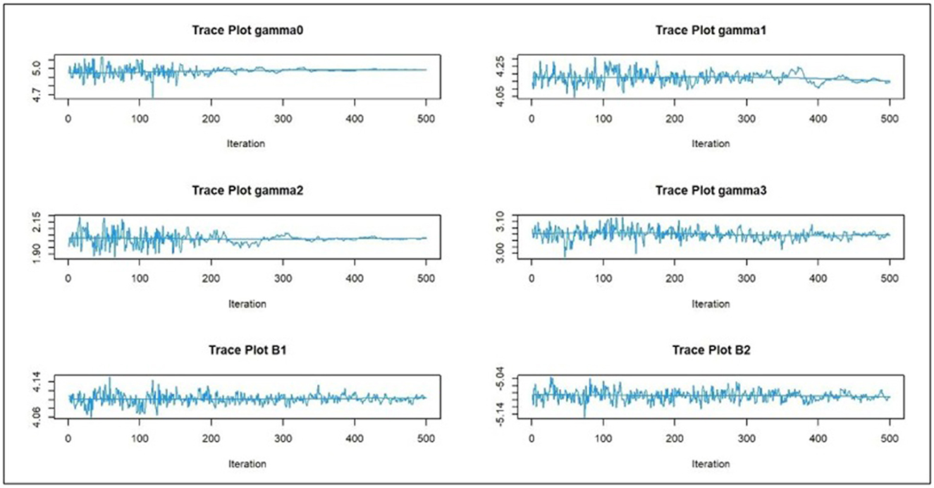
Figure 2. Sample of the trace plot for the SAEM estimates (n = 100), ετ,ij ~ ALD.
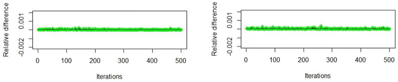
Figure 3. Sample of visual monitoring of the difference (relative difference) between two successive evaluations of the log-likelihood, ετ,ij ~ ALD.
For all scenarios, the absolute relative bias (ARB) for each parameter over the 1,000 replicates is obtained as , and the standard error for each estimator is obtained as , where is the Kth estimate of θ using the Kth sample and is the average of the multiple estimates, that is, .
Tables 1, 2 show the results of the simulations. We compare the performance of the proposed algorithm with the algorithm proposed by Li et al. [7]. We can conclude the following:
1. The proposed estimators are asymptotically unbiased for symmetric and skewed distributions. This is because the relative absolute bias of all estimates using the proposed algorithm is relatively small, as all values of ARB are < 0.2% of the value of the parameters, for both an ALD and the lognormal distributions. The result is valid for sample sizes n = 40 and 100.
2. It is clear that the ARB associated with most of the parameter estimates, for the proposed algorithm, is less than those of the algorithm proposed by Li et al. [7], when the errors follow an ALD or the lognormal distribution and sample sizes n = 40 and 100. This means that the proposed method is better than the algorithm proposed by Li et al. [7].
3. The proposed method is more efficient than the algorithm proposed by Li et al. [7].The standard errors of most of the estimators for the proposed algorithm are less than their counterparts of the algorithm proposed by Li et al. [7].
4. All the AIC values for the proposed technique are less than that for the model estimated by Li et al. [7].This means that the proposed algorithm outperforms the algorithm proposed by Li et al. [7].
5. According to the median absolute deviation values, the same conclusion can be derived as the MAD values for the proposed algorithm are less than that of the Li et al. [7] algorithm.
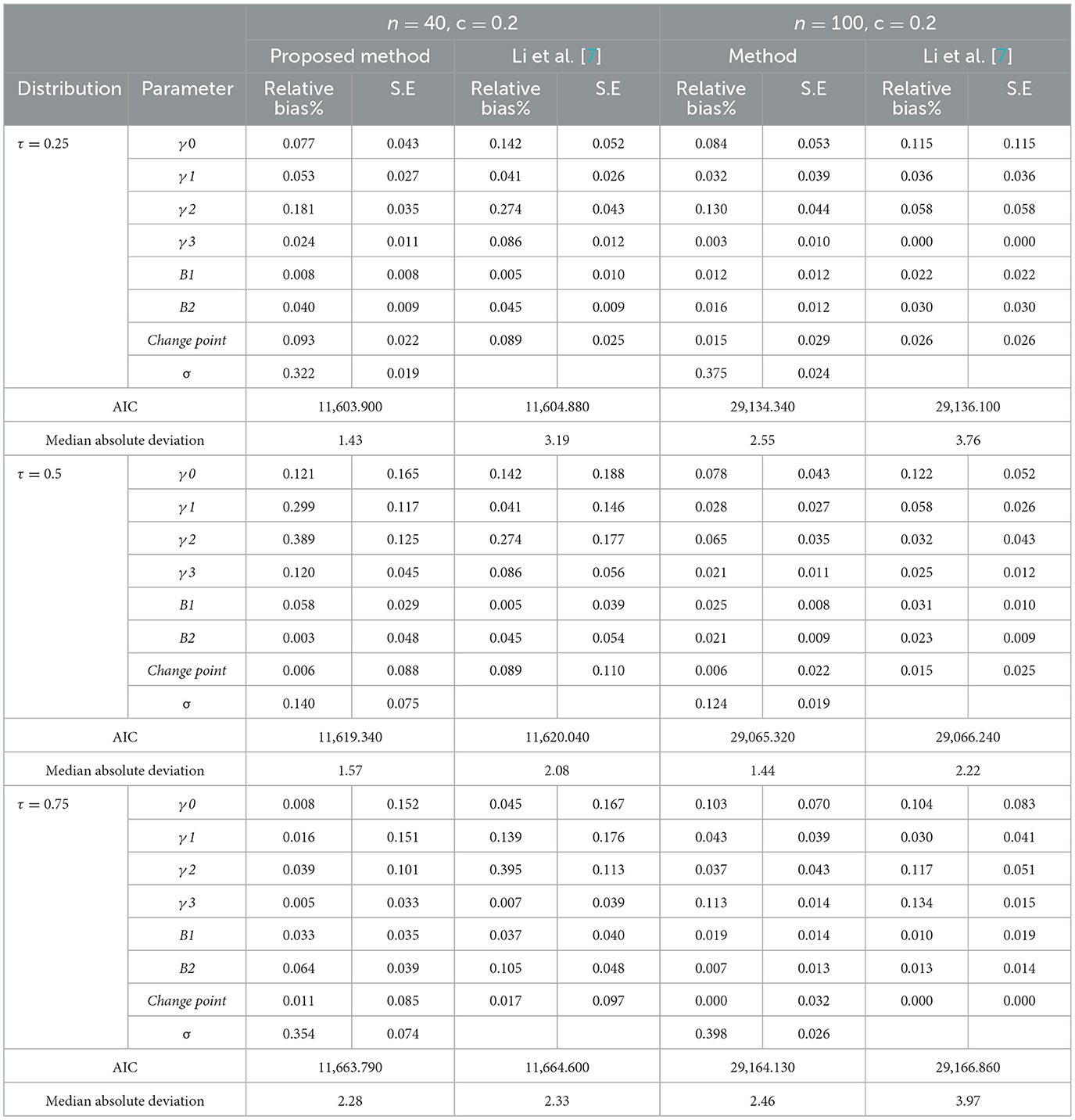
Table 1. Simulation results, the standard errors, and the relative bias for different models at n = 40, and 100, ετ,ij ~ ALD.
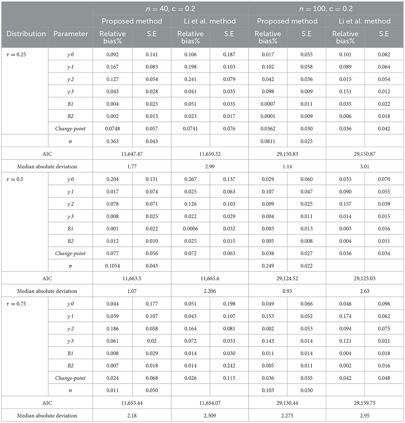
Table 2. Simulation results, the standard errors, and the relative bias for different models at n = 40, and 100, ετ,ij ~ Lognormal.
The first diagnosed case with COVID-19 symptoms is dated back to December 2019 in Wuhan city, China. COVID-19 affected the entire world, socially, economically, and even politically. There were more than 3 million deaths by the end of April 2021 as reported by the WHO. The factors that affect the spread of the disease, and the number of deaths, were the focus of many studies.
Studies have shown that environmental factors, in general, may affect the fast spread of COVID-19. Moreover, studies tried to investigate the impact of economic factors on virus transmission. A study on some Chinese cities during the period 19 January and 29 February of the year 2020 revealed that higher developed cities have high transmission rates. This may be due to the high economic activity that needs high social interactions [29].
The effect of demographic factors on the spread of COVID-19 was studied. Khan et al. [30] demonstrate that certain demographic attributes, such as the age distribution, the poverty ratio, the female smoker percentage, the obesity level, and the average annual temperature of the country, are significantly associated with COVID-19 death rate distribution.
In this article, we focus on global economic factors and health factors affecting the monthly death rate per million of COVID-19 to describe the spread and fatality of COVID-19 disease. We investigate whether there is a threshold effect (change point) in the relationship between the HDI and new monthly deaths per million. From Figure 4, we can conclude that the new deaths per million are skewed to the right. Thus, we need to focus on the factors that affect the lower and/or upper tails of the distribution of new deaths. However, most of the proposed statistical methodologies for describing longitudinal data with change points rely upon distributional assumptions that are not held in this case.
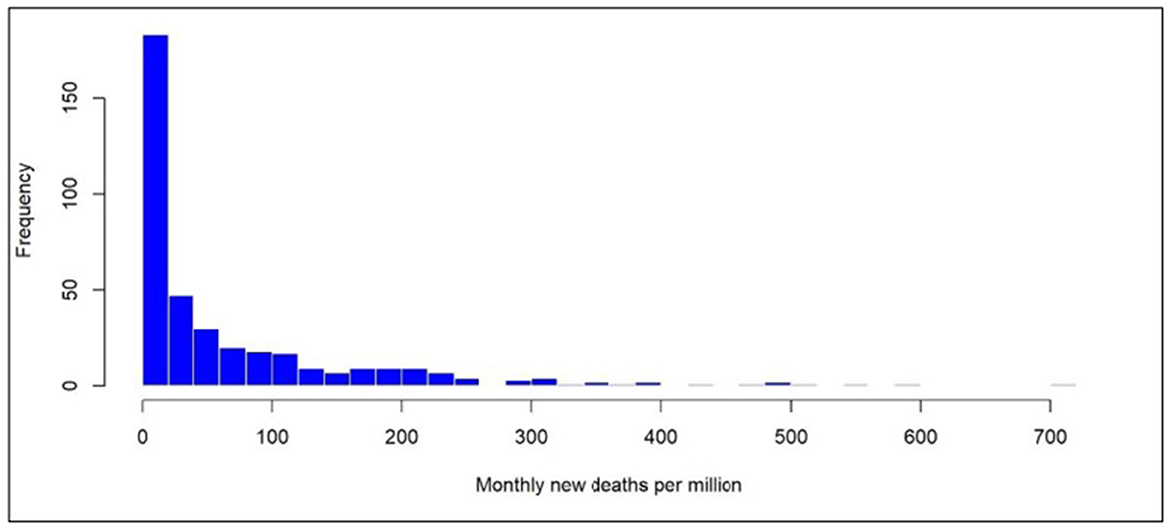
Figure 4. Histogram of the monthly new deaths per million.
The used data about the COVID-19 new deaths were obtained from the Our World In Data, an online (https://ourworldindata.org/coronavirus) publication. This cite has become one of the world's leading websites during the pandemic in 2020. The study focuses on the monthly data during the period starting from 1 April 2020 to 30 April 2021. The dependent variable is the new monthly deaths per million while the independent variables are as follows:
1- ICU: the monthly number of patients with COVID-19 in intensive care units (ICUs) on a given day per million.
2- The number of tests: the monthly tests conducted per new confirmed case of COVID-19.
3- Diabetes prevalence: Diabetes prevalence (% of the population aged 20–79) in 2017.
4- Hospital beds: The number of hospital beds per 1,000 people, most recent year available since 2010.
5- Median age: The median age of the population; UN projection for 2020.
6- Stringency index (SI): The government response stringency index; it is a composite measure based on nine response indicators, including school closures, workplace closures, and travel bans, rescaled to a value from 0 to 100 (100 is the strictest response).
7- HDI: A composite index measuring average achievement in three basic dimensions of human development; a long and healthy life, knowledge, and a decent standard of living values for 2019. It ranges from 0 to 1 in which 1 indicates higher development countries in the three aspects.
The 30 countries incorporated in the study are as follows:
Austria Bangladesh Brazil Bulgaria Canada
China Colombia Denmark Djibouti Dominican
Egypt Ethiopia Ghana Greece Hungary
India Iraq Ireland Italy Jordan
Kenya Morocco Portugal Russia Spain
Sweden Tunisia Turkey UK USA
These countries are chosen to represent different areas of the world according to the availability of the data. It is well mentioned that there are some countries suffering from missing data, especially in the variables monthly number of patients with COVID-19 in intensive care units (ICUs), and monthly tests conducted per newly confirmed cases of COVID-19. These values are imputed using the regression method. The variables that will be associated with the random effects are stringency index (SI), diabetes prevalence, and median age in addition to the intercept.
Table 3 presents the descriptive statistics of the variables in the study. Figure 5 presents the profile plot of the death rate for all countries over time, from it we can conclude that death distribution for all countries is skewed.
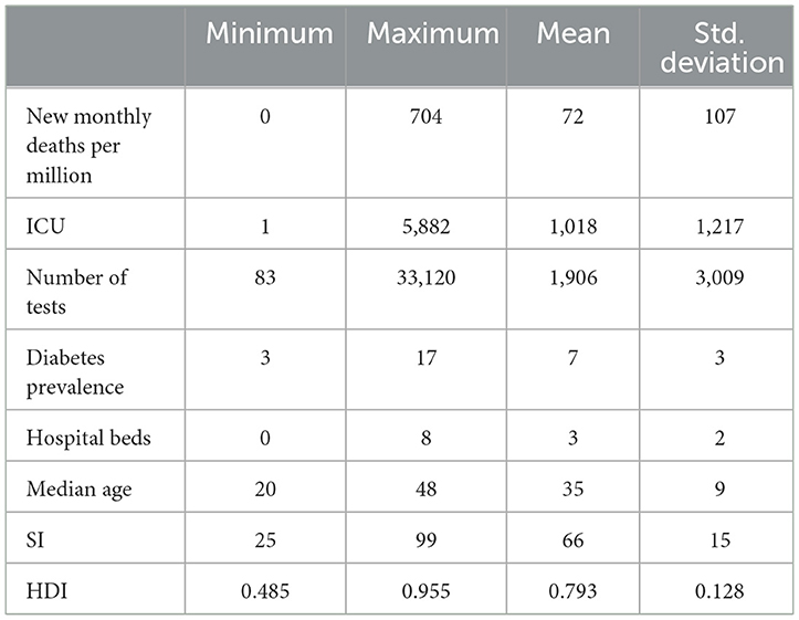
Table 3. Descriptive statistics of COVID-19 data.
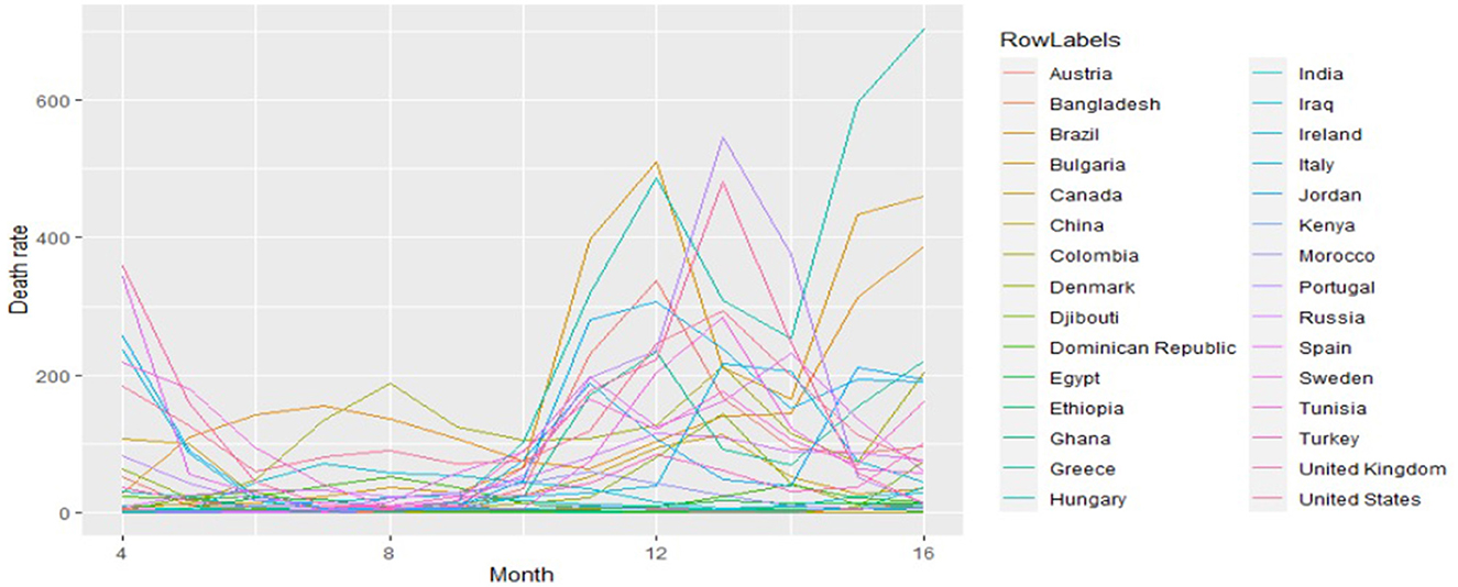
Figure 5. Spaghetti plot of new monthly deaths per million.
The aim of the data was to study the global economic and health factors that affect the monthly death rate due to COVID-19 from 1 April 2020 to 30 April 2021. As reported by the WHO, there are more than 3 million deaths due to COVID-19 by the end of April 2021. Many studies tried to understand the factors behind the spread of the disease and the factors that affect the number of deaths throughout the world. This enables us to minimize the losses faced due to COVID-19. Different factors are considered, in this article, including a composite index measuring average achievement in three basic dimensions of human development: a long and healthy life, knowledge, and a decent standard of living (HDI). The HDI ranges from 0 to 1, where 1 indicates higher human development in three dimensions.
Figure 6 shows a scatter plot of the relationship between the HDI and the new deaths per million. From Figure 6, we can see that there is a suspicion of having a threshold effect on the relationship between the HDI and the new monthly deaths per million. This is obvious, especially for mean regression, 25th percentile regression, and 80th percentile regression. Hence, the location of the change point may be at HDI between 0.7 and 0.8. This leads us to estimate the mixed effects quantile regression with a change point at 0.5th quantile and at 0.8th quantile.
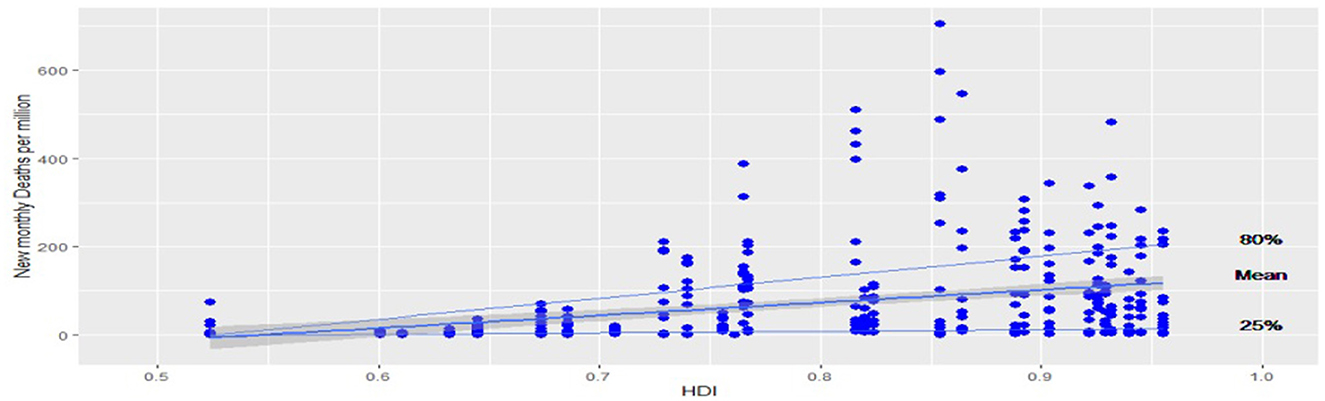
Figure 6. Scatter plot between HDI and monthly new deaths; the lines represent the fitted quantile regressions at 25th percentiles, 80th percentiles, and the fitted mean regression.
The proposed method was implemented at the quantiles τ = 0.5 and τ = 0.8 to test whether the HDI had any threshold effect on the monthly new deaths per million. The following model is fitted:
Where xij is the HDI, is a vector containing the observation of the following variables: ICU, number of tests, diabetes prevalence, hospital beds, median age, and stringency index (SI). The is a vector containing ones to represent the intercept, stringency index (SI), diabetes prevalence, and median age. The estimates of the fixed effect of the model and the location of the change point at τ = 0.5, using the proposed algorithm and the algorithm of Li et. al. [7] are summarized in Table 4. Moreover, the 95% confidence interval is obtained using the block bootstrap method with the number of replications equal to 1,000. From Table 4, depending on the confidence intervals, it is clear that there is a threshold effect in the relationship between the HDI and the new monthly deaths per million at HDI = 0.79 and 0.816, respectively. The effect of the HDI on the 0.5th quantile of new monthly deaths per million due to COVID-19 is 459.41 where this effect declines to 128.68 after the threshold is reached. Both effects are significant at a 95% confidence level. But for the 0.8th quantile we found that, prior to the threshold value, the effect of the HDI on the 0.8th quantile of new monthly deaths per million due to COVID-19 is 1414.293. This effect declines and has a negative value (-122.95) after the location of the threshold. This means that increasing the HDI affects the 0.5th quantile of new monthly deaths per million due to COVID-19 positively, before and after the threshold value. However, it affects the 0.8th quantile of new monthly deaths per million due to COVID-19 before the positive threshold value and after the negative threshold value.
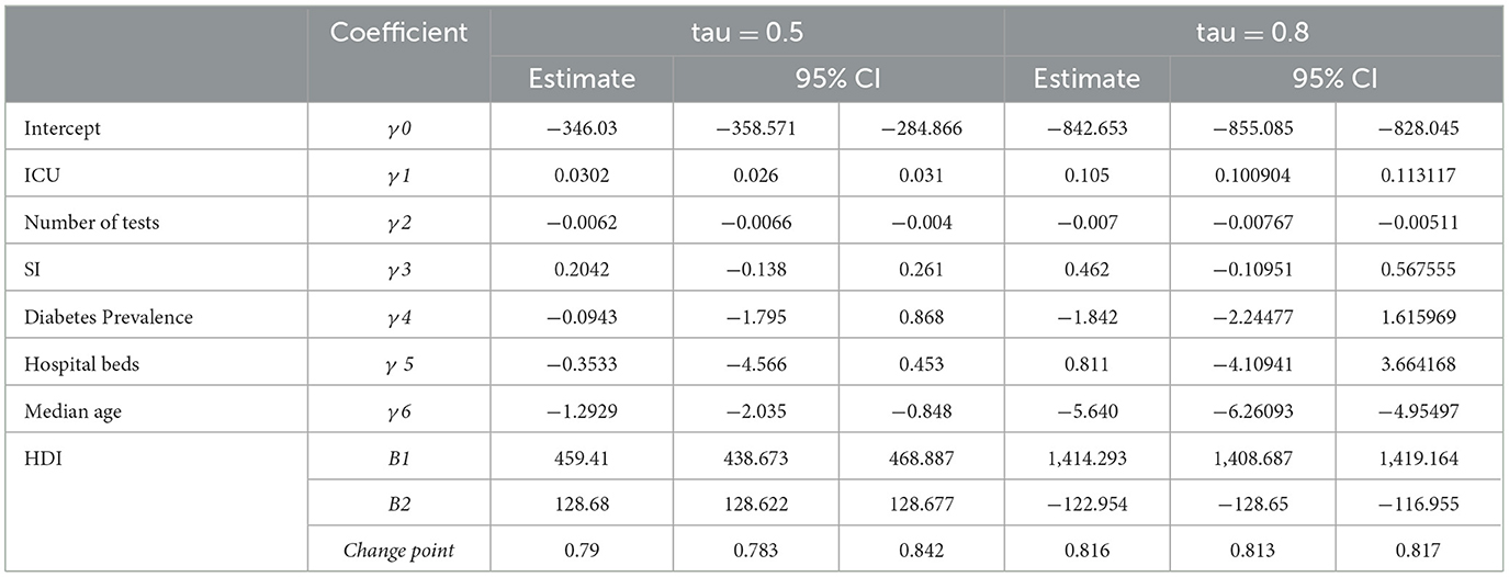
Table 4. Estimation of the mixed effects quantile change point regression model for COVID-19 data.
Furthermore, we can see that there is a positive effect of the monthly number of patients with COVID-19 in intensive care units (ICUs) for both 0.5th and 0.8th quantiles of new monthly deaths per million. This effect is greater in the case of the 0.8th quantile. There is a negative effect of each of the number of tests, and the median age of the population on both 0.5th and 0.8th quantiles of new monthly deaths per million. However, their effect is greater in the case of the 0.8th quantile. Each of the stringency index, hospital beds, and diabetes prevalence has no significant effect on both 0.5th and 0.8th quantiles of new monthly deaths per million due to COVID-19.
Table 5 presents the AIC values for the proposed model and the Li et al. [7] model at τ = 0.5 and 0.8. The results show that the proposed model performs better than the model of Li et al. [7].

Table 5. AIC and median absolute deviation values of the two models for COVID-19 data.
In this article, we propose the mixed effects quantile regression with a change point model for longitudinal data by relaxing the independence assumption. The mixed effects are used to capture the dependence structure of the longitudinal data. We use the stochastic approximation EM algorithm to estimate the parameters using the link between an asymptotic Laplace distribution and the quantile regression. In addition, the location of the change point is estimated using optimization methods. Simulation studies are conducted to evaluate the proposed techniques. The simulation results show that the proposed techniques are better than those of Li et al. [7] in terms of the relative biases and the standard errors for symmetric and skewed distributions.
The proposed techniques are applied to a real dataset about COVID-19. We found that there is a threshold effect in the relationship between the HDI and the 0.5th and 0.8th quantiles of new monthly deaths per million. Moreover, the results show a positive effect on the monthly number of patients with COVID-19 in intensive care units (ICUs) for both 0.5th and 0.8th quantiles of new monthly deaths per million. There is a negative effect of each of the number of COVID-19 tests and the median age of the population on both 0.5th and 0.8th quantiles of new monthly deaths per million. The stringency index, hospital beds, and diabetes prevalence have no significant effect on both 0.5th and 0.8th quantiles of new monthly deaths per million.
The proposed techniques are for complete longitudinal data and one change point. A new venue for future research is to extend the proposed techniques for longitudinal data with missing values. Another future research point is to modify the proposed methods to accommodate multiple change points. These points are under consideration by the researchers.
Publicly available datasets were analyzed in this study. This data can be found here: https://ourworldindata.org/coronavirus.
AG has introduced the idea of the research and review the results, also help in editing the manuscript. A-EA-R has reviewed the idea and help in the change point part and help in editing the article. WI has written the codes, tried the necessary modifications, and the simulation and application part. All authors contributed to the article and approved the submitted version.
The authors would like to thank the editor and reviewers for their constructive and helpful comments that significantly improved the article.
The authors declare that the research was conducted in the absence of any commercial or financial relationships that could be construed as a potential conflict of interest.
All claims expressed in this article are solely those of the authors and do not necessarily represent those of their affiliated organizations, or those of the publisher, the editors and the reviewers. Any product that may be evaluated in this article, or claim that may be made by its manufacturer, is not guaranteed or endorsed by the publisher.
The Supplementary Material for this article can be found online at: https://www.frontiersin.org/articles/10.3389/fams.2023.1106958/full#supplementary-material
1. Gad AM. Ibrahim WIM. An adaptive linear regression approach for modeling heavy-tailed longitudinal data. Commun. Stat. Simulat. Computat. (2020) 49:1181–97. doi: 10.1080/03610918.2018.1491990
2. Yang L. Gao S. Bivariate random change point models for longitudinal outcomes. Stat. Med. (2012) 32:1038–53. doi: 10.1002/sim.5557
3. Ghosh P. Vaida F. Random Changepoint modeling of HIV immunologic responses. Stat. Med. (2007) 26:2074–87. doi: 10.1002/sim.2671
4. Mclain A. Albert P. Modeling longitudinal data with a random change point and no time-zero: applications to inference and prediction of the labor curve Biometrics. (2014) 70:1052–60. doi: 10.1111/biom.12218
5. Xing H. Ying Z. A semiparametric change-point regression model for longitudinal data. J Am Statistic Assoc. (2012) 107:1625–37. doi: 10.1080/01621459.2012.712425
6. Lai Y. Albert P. Identifying multiple change-points in a linear mixed effects model. Stat Med. (2014) 33:1015–28. doi: 10.1002/sim.5996
7. Li C, Dowling N. Chappell R. Quantile regression with a change-point model for longitudinal data: an application to the study of cognitive changes in preclinical alzheimer's disease. Biometrics. (2015) 71:625–35. doi: 10.1111/biom.12313
8. Jung S., Quasi-likelihood for median regression models. Am Stat Assoc. (1996) 91, 251–7. doi: 10.1080/01621459.1996.10476683
9. Wang HJ. Fygenson M. Inference for censored quantile regression. Annal Stat. (2009) 37:756–81. doi: 10.1214/07-AOS564
10. Li C, Wei Y, Chappell R, He X. Bent line quantile regression with application to an allometric study of land mammls' speed and mass. Biometrics. (2011) 67:242–9. doi: 10.1111/j.1541-0420.2010.01436.x
11. Sha N. On Testing the Change-point in the Longitudinal Bent Line Quantile Regression Model, Graduate school of Arts and sciences, Columbia University, Coulmbia (2011).
12. Yu K. Moyeed R. Bayesian quantile regression. Statistics Probabil Lett. (2001) 54:437–47. doi: 10.1016/S0167-7152(01)00124-9
13. Liu Y. Bottai M. Mixed-eefects models for conditional quantiles with longitudinal data. Int J Biostatistic. (2009) 5:28. doi: 10.2202/1557-4679.1186
14. Meza C, Osorio F, l RCruz D, Estimation in nonlinear mixed-effects models using heavy-tailed distributions. Stat Comput. (2012) 22:121–39. doi: 10.1007/s11222-010-9212-1
15. Kotz S, Kozubowski TJ, Podgórski K. The Laplace Distribution and Generalizations. A Revisit with Applications to Communications, Economics, Engineering, and Finance. Basel: Birkhäuser (2001).
16. Galarza CE, Lachos VH. Bandyopadhyay D. Quantile regression in linear mixed models: a stochastic approximation EM approach. Stat Interface. (2017) 10:471–82. doi: 10.4310/SII.2017.v10.n3.a10
17. Abd Elwahab HA, Kholy RB. Gad AM. Sensitivity analysis index for shared parameter models in longitudinal studies. Adv Applicat Statistics. (2019) 17:1–20. doi: 10.17654/AS05701,0001
18. Yaseen ASA. Gad AM. A stochastic variant of the EM algorithm to fit mixed (discrete and continuous) longitudinal data with nonignorable missingness. Commun Stat Theory Meth. (2020) 498:4446–67. doi: 10.1080/03610926.2019.1601223
19. Buchinsky M. Estimating the asymptotic covariance matrix for quantile regression models: a monte carlo study. J Econometr. (1995) 8:303–38. doi: 10.1016/0304-4076(94)01652-G
20. Lipsitz R, Fitzmaurice GM, Molenberghs G. Zhao LP. Quantile regression methods for longitudinal data with drop-outs: application to CD4 cell counts of patients infected with the human immunodeficiency virus. Appl Stat. (1997) 46:463–76. doi: 10.1111/1467-9876.00084
21. Andrews DWK. Buchinsky M. A three-step method for choosing the number of bootstrap repetitions. Econometrica. (2000) 68:23–52. doi: 10.1111/1468-0262.00092
22. Qiu Y, Chen X, Shi W. Impacts of social and economic factors on the transmission of coronavirus disease 2019. (COVID-19) in China. J Populat Econ. (2020) 33:1127–72. doi: 10.1007/s00148-020-00778-2
23. Khan W, Hussain A, Khan SA, Al-Jumailey M, Nawaz R. Liatsis P. Analyzing the impact of global demographic characteristics over the COVID-19 spread using class rule mining and pattern matching. Royal Soc Open Sci. (2021) 8:21. doi: 10.1098/rsos.201823
24. Yirga AA, Melesse SF, Mwambi HG. Ayele DG. Additive quantile mixed effects modeling with application to longitudinal CD4 count data. Scientific Rep. (2021) 11:25. doi: 10.1038/s41598-021-97114-9
25. Tian Y, Wang L, Tang M. Tian M. Weighted composite quantile regression for longitudinal mixed effects models with application to AIDS studies. Commun Stat Simulat Computat. (2021) 50:1837–53. doi: 10.1080/03610918.2019.1610440
26. Galarza CE, Castro LM, Louzada F. Lachos VH. Quantile regression for nonlinear mixed effects models: a likelihood based perspective. Stat Pap. (2020) 1:1281–307. doi: 10.1007/s00362-018-0988-y
27. Abdelwahab AS, Gad AM, Abdrabou AS. A CUSUM test for change point in quantile regression for longitudinal data, communications in statistics. Simulat Applicat. (2022) 22:p. To appear. doi: 10.1080/03610918.2022.2112600
29. Dempster AP, Laird NM. Rubin DB. Maximum likelihood from incomplete data via the EM algorithm. J Royal Stat Soc. (1977) 39:1–38. doi: 10.1111/j.2517-6161.1977.tb01600.x
Keywords: longitudinal data, change point model, COVID-19, mixed effects quantile regression, bent line quantile regression, missing data
Citation: Ibrahim WIM, Gad AM and Abd-Rabou A-ES (2023) A mixed effects changepoint quantile regression model for longitudinal data with application on COVID-19 data. Front. Appl. Math. Stat. 9:1106958. doi: 10.3389/fams.2023.1106958
Received: 24 November 2022; Accepted: 03 February 2023;
Published: 24 February 2023.
Edited by:
Han-Ying Liang, Tongji University, ChinaReviewed by:
Ferra Yanuar, Andalas University, IndonesiaCopyright © 2023 Ibrahim, Gad and Abd-Rabou. This is an open-access article distributed under the terms of the Creative Commons Attribution License (CC BY). The use, distribution or reproduction in other forums is permitted, provided the original author(s) and the copyright owner(s) are credited and that the original publication in this journal is cited, in accordance with accepted academic practice. No use, distribution or reproduction is permitted which does not comply with these terms.
*Correspondence: Ahmed M. Gad,  YWhtZWQuZ2FkQGZlcHMuZWR1LmVn
Disclaimer: All claims expressed in this article are solely those of the authors and do not necessarily represent those of their affiliated organizations, or those of the publisher, the editors and the reviewers. Any product that may be evaluated in this article or claim that may be made by its manufacturer is not guaranteed or endorsed by the publisher.
Research integrity at Frontiers
Learn more about the work of our research integrity team to safeguard the quality of each article we publish.