A mathematical and exploratory data analysis of malaria disease transmission through blood transfusion

Malaria is a mosquito-borne disease spread by an infected vector (infected female Anopheles mosquito) or through transfusion of plasmodium-infected blood to susceptible individuals. The disease burden has resulted in high global mortality, particularly among children under the age of five. Many intervention responses have been implemented to control malaria disease transmission, including blood screening, Long-Lasting Insecticide Bed Nets (LLIN), treatment with an anti-malaria drug, spraying chemicals/pesticides on mosquito breeding sites, and indoor residual spray, among others. As a result, the SIR (Susceptible—Infected—Recovered) model was developed to study the impact of various malaria control and mitigation strategies. The associated basic reproduction number and stability theory is used to investigate the stability analysis of the model equilibrium points. By constructing an appropriate Lyapunov function, the global stability of the malaria-free equilibrium is investigated. By determining the direction of bifurcation, the implicit function theorem is used to investigate the stability of the model endemic equilibrium. The model is fitted to malaria data from Benue State, Nigeria, using R and MATLAB. Estimates of parameters were made. Following that, an optimal control model is developed and analyzed using Pontryaging's Maximum Principle. The malaria-free equilibrium point is locally and globally stable if the basic reproduction number (R₀) and the blood transfusion reproduction number (R_α) are both less or equal to unity. The study of the sensitive parameters of the model revealed that the transmission rate of malaria from mosquito-to-human (β_mh), transmission rate from humans-to-mosquito (β_hm), blood transfusion reproduction number (R_α) and recruitment rate of mosquitoes (b_m) are all sensitive parameters capable of increasing the basic reproduction number (R₀) thereby increasing the risk in spreading malaria disease. The result of the optimal control shows that five possible controls are effective in reducing the transmission of malaria. The study recommended the combination of five controls, followed by the combination of four and three controls is effective in mitigating malaria transmission. The result of the optimal simulation also revealed that for communities or areas where resources are scarce, the combination of Long Lasting Insecticide Treated Bednets (u₂), Treatment (u₃), and Indoor insecticide spray (u₅) is recommended. Numerical simulations are performed to validate the model's analytical results.

1. Introduction

Malaria is a protozoan disease, and the intermediate host is a female Anopheles mosquito infected with Plasmodium falciparum, Plasmodium vivax, Plasmodium ovale, or Plasmodium malariae. In addition to the bite of an infected female Anopheles mosquito, malaria can also be transmitted by the donation of blood from a donor who is infected with the disease [1]. The World Health Organization (WHO) recommends screening blood donors for malaria in malaria-endemic areas [2]. Few blood banks in Sub-Saharan Africa have implemented malaria screening due to a lack of data on the cost-effectiveness of screening technology [3]. Blood is a special kind of organic fluid produced by living organisms that are vital to their existence and everyday functioning [4]. Transfusions of human blood will continue to be a clinically essential medical treatment for a long time since, despite medical advancements, humanity has not been able to manufacture a functioning substitute for human blood [5]. Because of injuries, operations, anemia, and problems during pregnancy, half of all people will require a blood transfusion at some point in their lives. Although blood transfusions have been used for centuries, they have also been linked to the spread of disease when inadequate checks are made on blood donations [6]. In Kitchen and Chiodini [7] and Hirigo et al. [8], it was established that every drop of blood collected in blood banks be tested for major Transfusion Transmitted Infections (TTIs) like Human Immunodeficiency Virus (HIV), hepatitis B virus (HBV), hepatitis C virus (HCV), and syphilis before transfusion.

According to available data, the global incidence and occurrence of transfusion-transmitted infected blood with malaria is around 100 cases per year, with the majority of cases being limited to endemic countries [9]. Having malaria in a donor blood sample increases the risk of transfusion-transmitted malaria in Sub-Saharan African nations [10]. Because malaria infection after transfusion may be due to either spontaneous infection (infection through bites from an infected female (Anopheles mosquito) or transfusion transmission, distinguishing between the two is difficult in regions where malaria is widespread. This explains why the number of infected blood transfusions among malaria patients in endemic countries is underreported. An expanding challenge brought on by worldwide travel and immigration is the transmission of the malaria parasite through blood donations. In malaria-endemic areas, it is therefore more difficult to devise an optimal method to limit the danger of transfusion-transmitted contaminated blood without needless exclusion of blood donation, which remains a subject of discussion.

About 76 percent of the Nigerian population lives in areas with high malaria transmission and 24 percent in areas with low malaria transmission [10]. The transmission season in the south may last all year, whereas it is only 3 months or less in the north. Because malaria is widespread in Nigeria, blood donors may be more susceptible to infection. Although there are established practices for malaria screening, which have been put on the test menus at blood banks, there is a risk of non-screening, according to World Health Organization [2]. Current strategies such as testing and screening of donor's blood in non-endemic countries were reviewed in Reesink [11] and Reesink et al. [12]. The results of the study revealed that the current measures are sufficient while also suggesting that surveillance of transfusion-transmitted malaria is necessary for the future. Most nations have established a stringent donor deferral system based on an individual's travel history. However, this policy is not optimal because of the fact that many healthy donors differ, which may result in donation loss because lengthy deferrals may discourage donors from returning [7]. The ideal malaria control plan for a country or region may therefore differ depending on the baseline malaria risk experienced by the donor and the recipient population in relation to the available resources [11].

Many studies have been conducted on the mechanisms of malaria transmission. Agusto et al. [13] studied a deterministic system of differential equations for the transmission of malaria. Their work investigates optimal strategies for controlling the spread of malaria disease using treatment, insecticide-treated bed nets, and the spray of mosquito insecticide. Blayneh et al. [14], studied the dynamics of a vector-transmitted disease using two deterministic models. A further study investigates the effects of prevention and treatment controls on malaria disease while keeping the implementation cost at a minimum. In Adeniyi and Aderele [15], a mathematical model for the dynamics of the Transfusion-Transmitted Malaria model with optimal control was studied. A recent study by Zhao and Liu [16] focused on dynamical behavior and optimal control of a vector-borne diseases model on bipartite networks, while mathematical modeling and projections of a vector-borne disease with optimal control strategies: a case study of the Chikungunya in Chad was discussed in Abboubakar et al. [17]. With the help of a seven-dimensional ordinary differential equation and non-linear forces of infection in the form of saturation incidence rates, Olaniyi and Obabiyi [10] modeled the transmission of malaria between humans and mosquitoes. It was shown that the presence of malaria-causing parasites triggers the production of antibodies in both humans and mosquitoes. The only way to combat a parasite invasion of the circulatory system is for humans to produce more antibodies. The affected person's immunological condition, including their general health and diet, also has a role in whether or not the disease progresses. Using a deterministic mathematical model, the effects of different sanitation strategies on malaria were analyzed in Oluyo and Adeniyi [18] and Oluyo and Adeniyi [19]. The results showed that the malaria model exhibits a backward bifurcation, suggesting that other criteria, such as maintaining adequate sanitation, are necessary for eradicating malaria beyond simply reducing R_m < 1. Improved hygienic conditions lead to fewer mosquito bites and thus fewer malaria cases. To better understand and combat malaria in communities, the team at [20] created and analyzed a model of the disease's transmission dynamics. It was determined qualitatively whether or not the model accounted for the timing of events. All of the studies mentioned above did not consider malaria acquired through transfusion, hence, the present study is aimed at studying the dynamics of transfusion-transmitted and vector-borne malaria while also investigating the efficacy of various intervention strategies for preventing the spread of transfusion-transmitted and mosquito-borne malaria. Some of these strategies are blood screening, Long-Lasting Insecticide Bed Nets (LLIN), treatment with anti-malaria drugs, spraying chemicals or pesticides on places where mosquitoes breed, and indoor residual spray.

This paper is organized as follows; Section 2 entails the mathematical formulation of the malaria transfusion transmitted model. In Section 3, the mathematical analysis of the model is sub-sectioned into Section 3.1 where the feasible region and well-posedness of the model are discussed, and Section 3.2, which focuses on the equilibrium analysis of the model. The basic reproduction number of the model is discussed in Section 3.3, stability analysis of the malaria model is the focus in Section 4 while Section 5, presents the optimal control problem and its solutions. The statistical data analysis is discussed in Section 6. Numerical simulations, discussion of results, and concluding remarks are presented in Section 7.

2. Mathematical formulation

The study uses a deterministic model to analyze the dynamics of malaria disease transmission dynamics taking into account transmissions via mosquitoes and blood transfusion. The overall human and mosquito populations at any given time t are given by N_h(t) and N_m(t), respectively. Further decomposition of N_h(t) and N_m(t) yield N_h(t) = S_h(t) + I_h(t) + R_h(t) and N_m(t) = S_m(t) + I_m(t), where S_h(t), I_h(t), R_h(t), S_m(t), and I_m(t) denote the susceptible humans, infected humans, recovered humans, susceptible mosquito, and infected mosquito classes, respectively.

The force of transmitting malaria infection from an infected mosquito to humans, λ_h(t) is given as the product of the transmission rate β_mh from an infected mosquito in I_m(t) compartment to the proportion of susceptible humans in S_h(t) compartment. This is written mathematically as

$\begin{array}{ll}{\lambda }_h(t)=\frac{{\beta }_{mh}{I}_m(t)}{N_h(t)}.& (2.1)\end{array}$

The recruitment and natural death rates of humans are given as b_h and μ_h, respectively. Humans who recovered from malaria infection progress to the susceptible class at rate δ with the recovery of humans given as π. Human mortality due to malaria occurs at rate σ.

The force of infection from human-to-mosquito, λ_m(t) is the multiplication of the transmission rate β_hm from an infected humans to a susceptible mosquito in S_m(t) class expressed as

$\begin{array}{ll}{\lambda }_m(t)=\frac{{\beta }_{hm}{I}_h(t)}{N_h(t)}.& (2.2)\end{array}$

Susceptible mosquitoes , S_m(t) are recruited at the rate b_m while both S_m(t) and I_m(t) classes are depopulated by natural death at rate μ_m.

To account for the force of infection as a result of blood transfusion, we have the term p₁αb_hI_h(t), where p₁ is the probability of effectively transfusing infected blood to a susceptible human, α is the transfusion term.

Consequently, within the scope of our analysis from this point on, the use of the time t dependency is suppressed. Given the submissions above, the discussion is presented in the following system of non-linear ordinary differential equations:

$\begin{array}{l}{S}_h^{\prime }=(1-p_1\alpha I_h)b_h-({\lambda }_h+{\mu }_h)S_h+\delta R_h,\hfill \\ I_h^{\prime }=p_1\alpha b_h{I}_h+{\lambda }_h{S}_h-A_0{I}_h,\hfill \\ R_h^{\prime }=\pi I_h-A_1{R}_h,\hfill \\ S_m^{\prime }=b_m-({\lambda }_m+{\mu }_m)S_m,\hfill \\ I_m^{\prime }={\lambda }_m{S}_m-{\mu }_m{I}_m,\hfill \end{array}(2.3)$

where A₀ = (σ + π + μ_h), A₁ = (δ + μ_h).

The model in Equation (2.3) above is based on the following assumptions:

(i) Malaria can be transmitted via infected mosquitoes and through transfusion of infected blood from a donor to a susceptible human;

(ii) The probability of survival till the infected stage for both humans and vectors is unity. Hence, the exposed compartments for both humans and vectors are not considered;

(iii) The term p₁αb_hI_h(t) is assumed to capture individuals who become infected with malaria due to transfusion.

3. Model dynamics

Let the total human population at any time t be N_h such that

$\begin{array}{ll}{N}_h=S_h+I_h+R_h.& (3.1)\end{array}$

The derivative of Equation (3.1) w.r.t t is

$\begin{array}{l}{N}_h^{\prime }=S_h^{\prime }+I_h^{\prime }+R_h^{\prime }=b_h-{\mu }_h{N}_h-\sigma I_h,\hfill \end{array}(3.2)$

since the term σI_h is non-negative, then

$\begin{array}{l}{N}_h^{\prime }\le b_h-{\mu }_h{N}_h.\hfill \end{array}(3.3)$

Thus, the solution of Equation (3.3) as t → ∞ yields

$\begin{array}{ll}{N}_h\le \frac{b_h}{{\mu }_h}.& (3.4)\end{array}$

Similarly, the total mosquito population is N_m

$\begin{array}{ll}{N}_m=S_m+I_m.& (3.5)\end{array}$

Thus, over time, the total mosquito population is

$\begin{array}{ll}{N}_m\le \frac{b_m}{{\mu }_m}.& (3.6)\end{array}$

3.1. Positivity and boundedness of solutions

The model (Equation 2.3) will be analyzed in the region

$\begin{array}{ll}\text{Ω}=\left\{\{(S_h,I_h,R_h,S_m,I_m)\in R_5^{+}:S_h+I_h+R_h\le \frac{b_h}{{\mu }_h},S_m+I_m\le \frac{b_m}{{\mu }_m}\right\},& (3.7)\end{array}$

Thus in this region, system (Equation 2.3) is mathematically and epidemiologically well-posed.

3.2. Equilibrium points

In this section, the general equilibrium point of the system (Equation 2.3) is considered. This is achieved by solving the system (Equation 2.3) at steady states. Particularly, system (Equation 2.3) have the general equilibrium denoted by M^⋆ as:

$\begin{array}{ll}{M}^{\star }=1.4\{\begin{array}{l}{S}_h^{*}=\frac{A_0{A}_1{b}_h(1-R_{\alpha })}{(A_2{\lambda }_h^{*}+A_3)},\\ I_h^{*}=\frac{A_1{b}_h{\lambda }_h^{*}}{A_2{\lambda }_h^{*}+A_3},\\ R_h^{*}=\frac{\pi b_h{\lambda }_h^{*}}{A_2{\lambda }_h^{*}+A_3},\\ S_m^{*}=\frac{b_m}{{\lambda }_m^{*}+{\mu }_m},\\ I_m^{*}=\frac{b_m{\lambda }_m^{*}}{{\mu }_m({\lambda }_m^{*}+{\mu }_m)},\end{array}& (3.8)\end{array}$

where

$\begin{array}{ll}{R}_{\alpha }=\frac{p_1\alpha b_h}{A_0}.& (3.9)\end{array}$

Details of how M^⋆ is obtained are given in the Appendix. To be precise, the following feasible steady states are obtained:

(i) Malaria Free Equilibrium (MFE) denoted by M₀. This depicts the solution of system (Equation 2.3) corresponding to the scenario where there is no presence of malaria disease (whether mosquito or blood transfusion induced) in the population. The feasibility of M₀ depends on whether the thresholds R_α and R₀ corresponding to the blood transfusion-induced reproduction number and the basic reproduction number are less than unity or otherwise. Hence,

$\begin{array}{l}{M}_0=(S_{h0},I_{h0},R_{h0},S_{m0},I_{m0})=\left(\frac{b_h}{{\mu }_h},0,0,\frac{b_m}{{\mu }_m},0\right),\hfill \end{array}(3.10)$

where

$\begin{array}{ll}{R}_0=\sqrt{\frac{{\beta }_{hm}{\beta }_{mh}{b}_m{\mu }_h}{{\mu }_m^2{b}_h{A}_0(1-R_{\alpha })}}.& (3.11)\end{array}$

In the following section, a detailed explanation of the thresholds R_α and R₀ is provided.

(ii) Malaria Endemic Equilibrium (MEE) written as M^⋆ in Equation (3.8) is a situation where malaria disease transmission persists in the population and is only possible if R_α < 1 and R₀ > 1

Remarks 1. Detailed calculations on the determination of the equilibrium points in (3.8) and (3.10) are given in the Appendix.

3.3. Analysis of the basic reproduction number, R₀

R_α and R₀ are thresholds called the blood transfusion-induced reproduction number and the basic reproduction number, respectively. R_α and R₀ represent the average number of secondary infections caused by transfusing infected blood to a susceptible human or a single infected mosquito when introduced into a population of only susceptible. R_α captures the dynamics of the model when malaria disease is transmitted via infected blood transfusion while R₀ represents the dynamic of the model whenever malaria is propagated through an infected vector. The theory on the calculation of the basic reproduction number R₀ is popularly based on the next-generation method explained in Diekmann et al. [21] and Van den Driessche and Watmough [22] and implemented in Adeniyi et al. [23, 24] and Chukwu et al. [25].

Studies in Olabisi and Olaniyi [19] and Buonomo and Lacitignola [26] have shown that for disease eradication, reducing the basic reproduction number below unity may not be sufficient, rather it may depend on other parameters or thresholds such as R_α as we have in this case. For a good insight into the thresholds R_α and R₀, we shall decompose the expressions for R_α and R₀ to see how they both and individually impact malaria transmission. It is easy to decompose R₀ into:

$\begin{array}{l}{R}_0=\sqrt{\frac{{\mu }_h}{b_h}}\sqrt{\frac{{\beta }_{mh}}{(\sigma +\pi +{\mu }_h)}}\sqrt{\frac{{\beta }_{hm}}{{\mu }_m}}\sqrt{\frac{b_m}{{\mu }_m}}\sqrt{\frac{1}{(1-R_{\alpha })}},\end{array}$

which can be written compactly as

$\begin{array}{ll}{R}_0=\sqrt{R_i},i=1,2,...5.& (3.12)\end{array}$

We explain below how each factor of Equation (3.12) impacts the basic reproduction number R₀, thereby giving us an insight on the disease control :

(i) The first quantity of Equation (3.12), $R_1=\frac{{\mu }_h}{b_h}$, i.e the ratio of the human natural death rate to the human recruitment rate, is normally less than unity since recruitment rate of humans b_h is always greater than natural death rate μ_h, thus the quantity R₁ will not increase the reproduction number, R₀.

(ii) The second quantity, $R_2=\frac{{\beta }_{mh}}{(\sigma +\pi +{\mu }_h)}$ is monotonically decreasing with regards to humans malaria induced mortality, σ plus the human recovery rate from malaria and the natural mortality rate in humans, is always greater than zero. This submission is true if the transmission of malaria from mosquito to humans is less than one and the denominator of R₂ increases. As this may sound, increasing σ and μ_h is not realistic in a real-life scenario, hence, the quantity R₂ provides no control over R₀.

(iii) The term $R_3=\frac{{\beta }_{hm}}{{\mu }_m}$ is a critical quantity that must be controlled to ensure R₀ is not increased. This is because the human-to-mosquito transmission probability, β_hm is always greater compared to the vector natural death rate μ_m, thus R₃ > 1 which implies R₃ will increase R₀.

(iv) From other studies , $R_4=\frac{b_m}{{\mu }_m}$ is greater than unity since b_m > μ_m, thus R₄ will produce a positive effect on R₀. This implies that decreasing the recruitment rate and increasing the fatality rate of the mosquitoes will provide good control.

(v) R_α captures the contribution of humans infected with malaria through blood transfusion. For R_α < 1, the quantity $R_5=\frac{1}{(1-R_{\alpha })}>1$ impact R₀ positively, therefore, the quantity R₅ should be controlled by ensuring R_α → 0.

The impact of each parameter in the basic reproduction number, R₀ also provides insight into which parameters should be controlled in order to interrupt the transmission of malaria, and is discussed below:

1. The transmission probability from mosquito to human, β_mh as shown in Figure 1A increases the basic reproduction number, R₀. Thus, it is important to mitigate this by ensuring that effective strategies such as the use of insecticide spray and sleeping under Long-Lasting Insecticide Treated Bednets (LLITBs) are in place to reduce the contact between humans and mosquitoes.

2. β_hm, denote the transmission probability of infection from human-to-mosquito. The basic reproduction number, R₀ increases as β_hm increases (see Figure 1B) which suggest that this parameter must be controlled. Just as in the of β_mh, the use of controls such as insecticide spray and the of LLINs should be encouraged.

3. In Figure 1C, the impact of R_α on R₀ is shown. R_α is the reproduction number for malaria acquired through blood transfusion. If R_α is allowed to increase, it will lead to an increase in the basic reproduction number, R₀, hence control such as blood screening must be ensured to reduce the risk of transfusing infected blood to susceptible humans.

4. The recruitment rate of susceptible mosquitoes, b_m will increase R₀ as shown in Figure 1D. This is indeed the case if mosquitoes are allowed to breed freely in the environment and humans are exposed to malaria-infected humans, then the chances that more susceptible mosquitoes may become infected are very high, thus leading to the spread of malaria disease through the mosquitoes' quest for blood meals from humans. Given this, it is important to control the mosquito's recruitment rate, b_m to ensure R₀ is brought below unity.

5. π denotes the recovery rate of humans after treatment from malaria bouts. The recovery rate π is critical in the control of malaria disease. As shown in Figure 2B, π will reduce the basic reproduction number, R₀.

6. μ_m, represent the natural mortality rate of mosquitoes. As displayed in Figure 2C, an increase in μ_m results in a decrease in R₀. This is a clear indication that strategies that will effectively increase the mortality rate of the mosquitoes such as pesticide spray and larvicide spray on mosquitoes and larva breeding sites are suggested.

7. As shown in Figure 2D, the parameter σ which signifies malaria-induced death rate decreases the basic reproduction number R₀ as σ increases, however, this is unrealistic and hence, it cannot be used to control R₀ and thus the disease spread.

8. As shown in Figure 2A, increasing the natural death rate μ_h of humans decreases R₀ significantly, this is not practical in a real-life scenario, thus, μ_h does not provide any control R₀ and disease control.

FIGURE 1

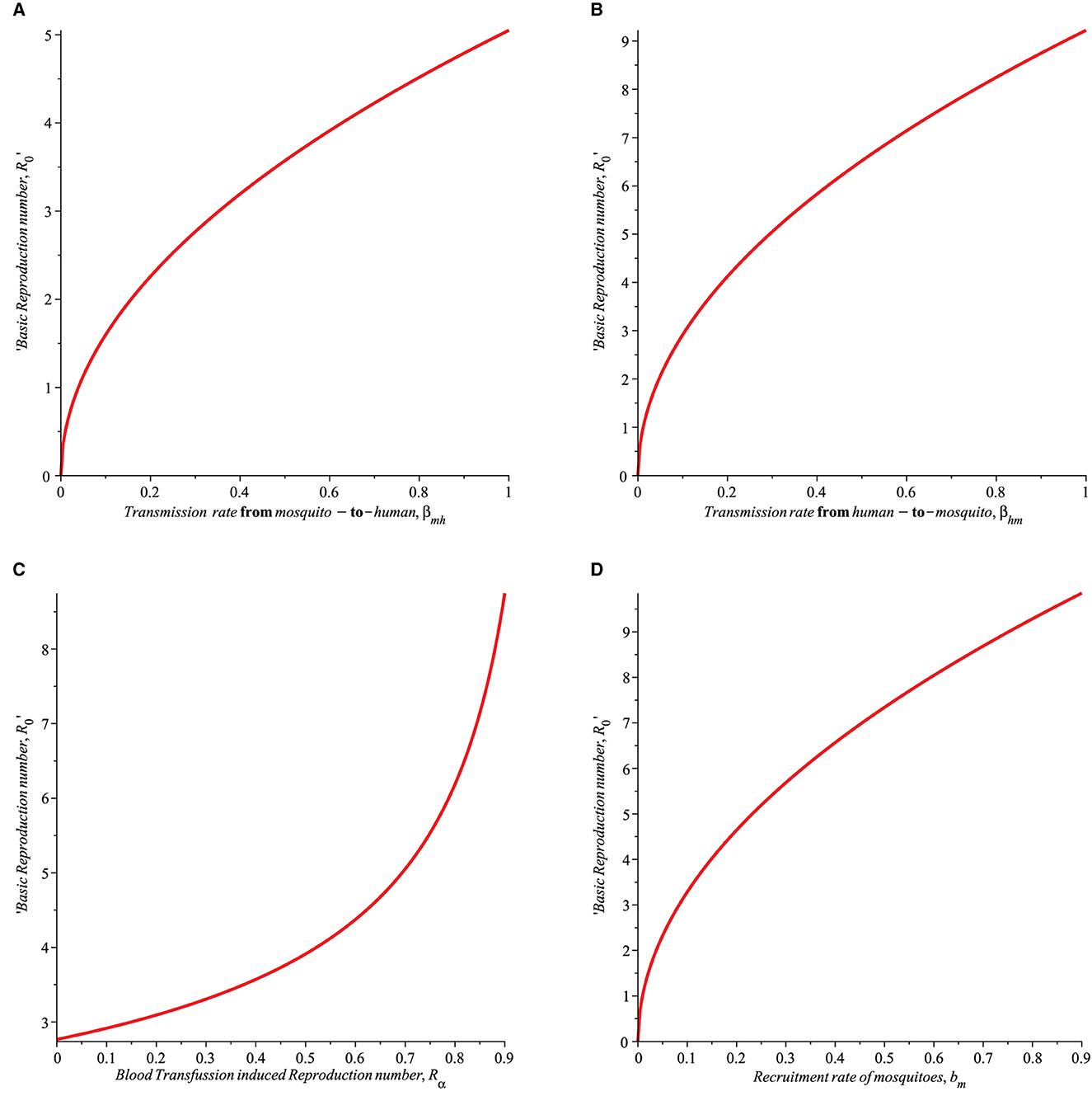
Figure 1. Simulation showing the impact of (A) transmission rate from mosquito-to-humans (β_mh), (B) transmission rate from human-to-mosquito (β_hm), (C) transfusion induced reproduction number (R_α), and (D) recruitment rate of mosquitoes (b_m) on the basic Reproduction number (R₀) with parameters set given in Table 1.

FIGURE 2

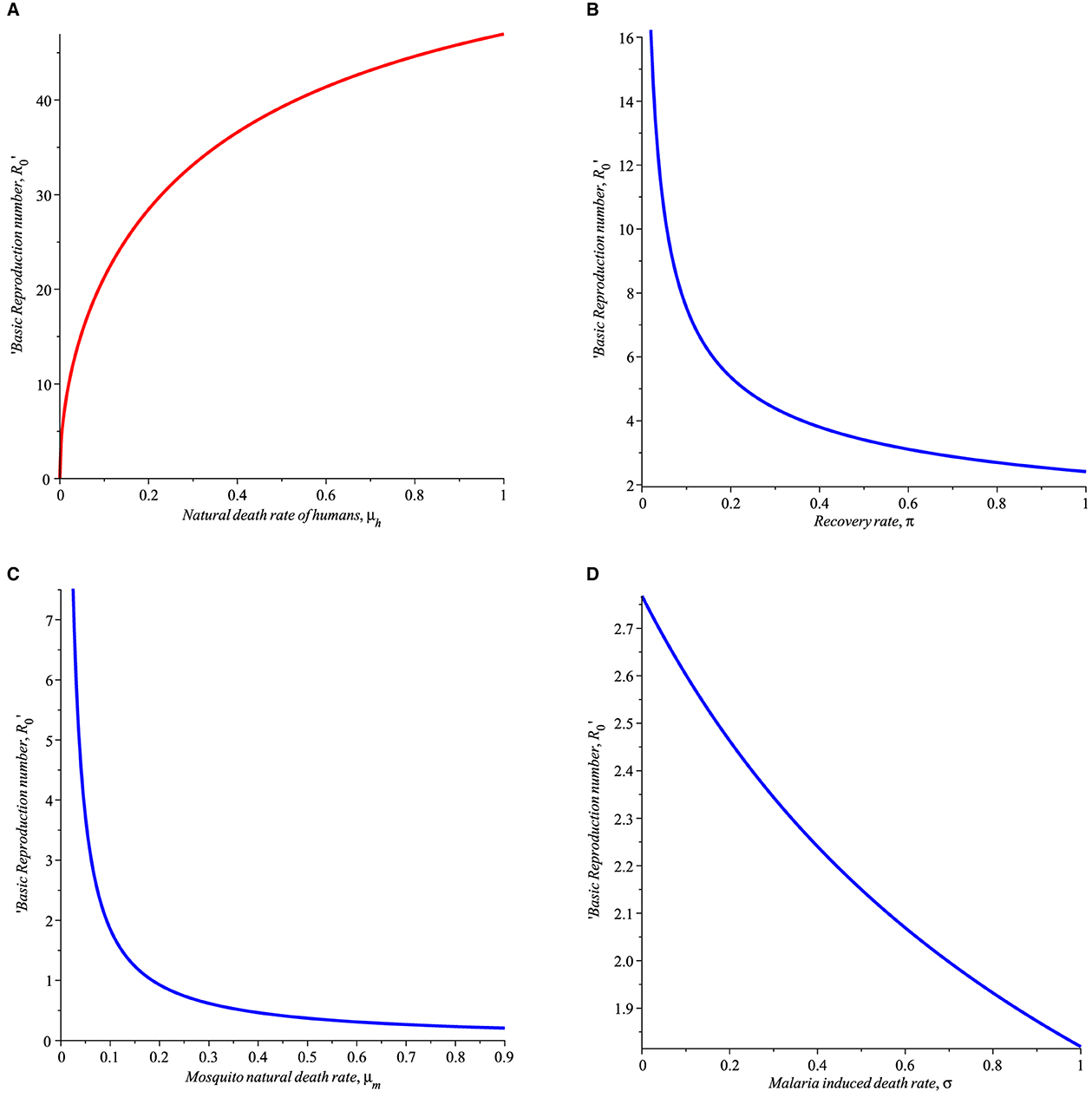
Figure 2. Simulation showing the impact of (A) natural death rate of humans (B) human recovery rate from malaria (π), (C) mortality rate of mosquitoes (μ_m), (D) malaria induced death rate (σ) with parameters set given in Table 1.

In Figure 3, varying values of the transfussion term α is simulated to see the impact on the susceptible humans, infected humans, recovered humans, and infected mosquitoes. It can be seen from Figure 3 that as α increases more individual become susceptible to malaria leading to increase in the number of infected humans recovered individuals. In Figure 3D, the number of infected mosquitoes also increased as α increases.

FIGURE 3

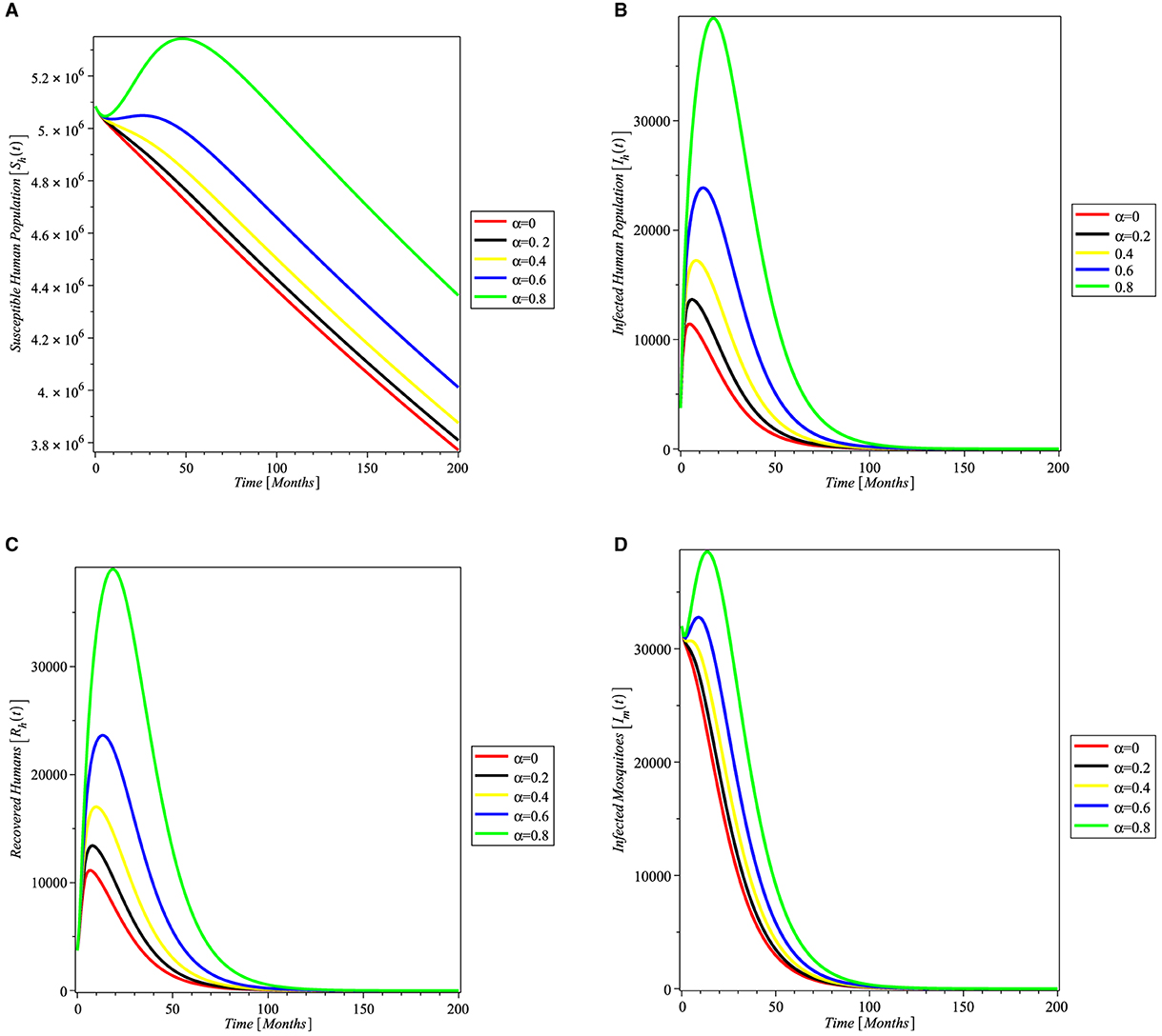
Figure 3. Simulation showing the impact of transfusion term alpha on (A) susceptible humans, (B) infected humans, (C) recovered humans, and (D) infected mosquitoes, with parameters set given in Table 1.

Following the above discussion, the optimal control of the model will be studied in Section 5 taking into account the impact of the parameters on the basic reproduction number, R₀.

4. Stability analysis of the model

4.1. Local stability analysis of malaria free equilibrium, M₀

When ${\lambda }_h^{*}={\lambda }_m^{*}=0$ in (3.8) yield the malaria-free equilibrium denoted by M₀,

$\begin{array}{ll}\begin{array}{l}{M}_0=(S_{h0},I_{h0},R_{h0},S_{m0},I_{m0})=\left(\frac{b_h}{{\mu }_h},0,0,\frac{b_m}{{\mu }_m},0\right)\hfill \end{array}& (4.1)\end{array}$

The Jacobian matrix of system (2.3) at M₀ is

$\begin{array}{ll}\begin{array}{l}J(M_0)=\left(\begin{array}{ccccc}-{\mu }_h& -\alpha p_1{b}_h& \delta & 0& -{\beta }_{mh}\\ 0& -A_0(1-R_{\alpha })& 0& 0& {\beta }_{mh}\\ 0& \pi & -A_1& 0& 0\\ 0& \frac{-{\beta }_{hm}{\mu }_h{b}_m}{b_h{\mu }_m}& 0& -{\mu }_m& 0\\ 0& \frac{{\beta }_{hm}{\mu }_h{b}_m}{b_h{\mu }_m}& 0& 0& -{\mu }_m\end{array}\right)\hfill \end{array}& (4.2)\end{array}$

It is easy to see that the eigenvalues of Equation (4.2) are λ₁ = −μ_h, λ₂ = −A₁ and λ₃ = −μ_m with the other two obtained from the 2 × 2 matrix M namely:

$\begin{array}{ll}\begin{array}{l}M=\left(\begin{array}{cc}-A_0(1-R_{\alpha })& {\beta }_{mh}\\ \frac{{\beta }_{hm}{\mu }_h{b}_m}{b_h{\mu }_m}& -{\mu }_m\end{array}\right).\hfill \end{array}& (4.3)\end{array}$

By Routh-Hurwithz condition [27], the eigenvalues of M are real negative if (i)Tr(M) < 0 and (ii)Det(M) > 0. Simple manipulation shows that

$\begin{array}{ll}Tr(M)=-A_0(1-R_{\alpha })-{\mu }_m<0if{R}_{\alpha }<1,& (4.4)\end{array}$

and

$\begin{array}{l}Det(M)={\mu }_m{A}_0(1-R_{\alpha })-\frac{{\beta }_{mh}{\beta }_{hm}{\mu }_h{b}_m}{b_h{\mu }_m},\\ ={\mu }_m{A}_0(1-R_{\alpha })\left(1-\frac{{\beta }_{mh}{\beta }_{hm}{\mu }_h{b}_m}{b_h{\mu }_m^2{A}_0(1-R_{\alpha })}\right),\\ ={\mu }_m{A}_0(1-R_{\alpha })(1-R_0^2).& (4.5)\end{array}$

Thus, the two eigenvalues of M are negative. Hence, the eigenvalues of Equation (4.2) are real and negative if R₀ < 1 and R_α < 1 thus establishing that the malaria free equilibrium, M₀ is locally asymptotically stable if R₀ < 1 and R_α < 1, otherwise unstable. The foregoing discussion is summarized in the following theorem:

Theorem 1. The malaria free equilibrium M₀ of system (Equation 2.3) is locally asymptotically stable if R₀ < 1 and R_α < 1, otherwise unstable.

Remark 1. R₀ is the basic reproduction number representing the average number of secondary infections caused by transfusing infected blood to a susceptible human or a single infected mosquito when introduced into a population of only susceptibles.

4.2. Global stability analysis of malaria free equilibrium, M₀

Suppose the stability of M₀ does not depend on the initial size of the infected population, then it is important to consider the global stability of M₀ of the system (Equation 2.3). This is motivated through the method of Lyapunov function [28]. The Lyapunov function technique has been widely used by many researchers [10, 20] to prove the global stability of equilibrium points.

Let us consider a Lyapunov function defined as follows:

$\begin{array}{l}L(I_h,I_m)={\mu }_m{I}_h+{\beta }_{mh}{I}_m,\end{array}(4.6)$

then the derivative of Equation (5.12) yield

$\begin{array}{l}{L}^{\prime }(I_h,I_m)={\mu }_m{I}_h^{\prime }+{\beta }_{mh}{I}_m^{\prime }.\hfill \end{array}(4.7)$

Taking into account of the values of $I_h^{\prime }$ and $I_m^{\prime }$ from Equation (2.3), then Equation (4.7) lead to

$\begin{array}{l}\begin{array}{l}{L}^{\prime }(I_h,I_m)={\mu }_m[\frac{{\beta }_{mh}{I}_m{S}_h}{N_h}+p_1\alpha b_h{I}_h-A_0{I}_h]\hfill \\ \begin{array}{l}+{\beta }_{mh}[\frac{{\beta }_{hm}{I}_h{S}_m}{N_h}-{\mu }_m{I}_m]\hfill \end{array}\hfill \end{array}\hfill \end{array}(4.8)$

After expanding and rearranging, then

$\begin{array}{l}{L}^{\prime }(I_h,I_m)={\mu }_m{A}_0(\frac{p_1\alpha b_h}{A_0}+\frac{{\beta }_{mh}{\beta }_{hm}{S}_m}{{\mu }_m{A}_0{N}_h}-1)I_h\hfill \\ +(\frac{{\mu }_m{\beta }_{mh}{S}_h}{N_h}-{\mu }_m{\beta }_{mh})I_m,\hfill \end{array}$

so that at DFE, $M_0\Rightarrow S_h=N_h=\frac{b_h}{{\mu }_h}\mathrm{\text{and }}{S}_m=\frac{b_m}{{\mu }_m}$. Thus,

$\begin{array}{l}{L}^{\prime }(I_h,I_m)={\mu }_m{A}_0(\frac{p_1\alpha b_h}{A_0}+\frac{{\beta }_{mh}{\beta }_{hm}{b}_m{\mu }_h}{{\mu }_m^2{A}_0{b}_h}-1)I_h,\hfill \\ ={\mu }_m{A}_0(R_{\alpha }+(1-R_{\alpha })R_0^2-1)I_h,\hfill \\ ={\mu }_m{A}_0(R_{\alpha }-1)(1-R_0^2).\hfill \end{array}(4.9)$

Hence, for R₀ ≤ 1, and R_α ≤ 1, then $L^{\prime }(I_h,I_m)\le 0$. This implies that the malaria-free equilibrium, M₀ is globally asymptotically stable if R₀ ≤ 1 and R_α ≤ 1, otherwise unstable.

4.3. Stability analysis of the endemic equilibrium M^* and bifurcation

If R₀ > 1 when conditions that favor disease thrive in the host population, then an endemic equilibrium may emerge. More importantly, it is crucial and necessary to carefully study the stability of the malaria endemic equilibrium M^* by considering the direction of bifurcation whether it is sub-critical or trans-critical. Bifurcation is a phenomenon that describes a situation where both the disease-free equilibrium and the endemic equilibrium co-exist. The method of implicit function theorem [29] is invoked to investigate this scenario.

Firstly, let α = α^* be a bifurcation parameter at R₀ = 1, then

$\begin{array}{ll}\alpha ={\alpha }^{*}=\frac{A_0{\mu }_m^2{b}_h-{\beta }_{mh}{\beta }_{hm}{b}_m{\mu }_m}{{\mu }_m^2{b}_h^2{p}_1}.& (4.10)\end{array}$

Let the infected component of the system (Equation 2.3) be denoted by m and m₀ be the jacobian matrix of the infected components of the system (Equation 2.3) evaluated at $(M_0,{\alpha }^{*})$ be defined respectively as

$\begin{array}{l}m=\left(\begin{array}{cc}{p}_1\alpha b_h-A_0& \frac{{\beta }_{mh}{S}_h}{{\mu }_h}\\ \frac{{\beta }_{hm}{S}_m}{{\mu }_h}& -{\mu }_m\end{array}\right)\hfill \end{array}$

and

$\begin{array}{l}{m}_0=\left(\begin{array}{cc}\frac{-{\beta }_{mh}{\beta }_{hm}{b}_m{\mu }_h}{b_h{\mu }_m^2}& {\beta }_{mh}\\ \frac{{\beta }_{hm}{b}_m{\mu }_h}{b_h{\mu }_m}& -{\mu }_m\end{array}\right),\hfill \end{array}$

With the following eigenvalues ${\lambda }_1=0\mathrm{\text{ and }}{\lambda }_2=-\frac{b_h{\mu }_m^3+{\beta }_{mh}{\beta }_{hm}{b}_m{\mu }_h}{b_h{\mu }_m^2}$ at α^*. Thus, λ₁ = 0 is a simple zero eigenvalue. Furthermore, denote by $w={(w_1,w_2)}^T$ a right eigenvector associated with λ₁ = 0. It follows that

$\begin{array}{ll}-\frac{{\beta }_{mh}{\beta }_{hm}{b}_m{\mu }_h}{b_h{\mu }_m^2}{w}_1+{\beta }_{mh}{w}_2=0,& (4.11)\end{array}$

$\begin{array}{ll}-\frac{{\beta }_{hm}{b}_m{\mu }_h}{b_h{\mu }_m}{w}_1+{\mu }_m{w}_2=0.& (4.12)\end{array}$

It follows from Equation (4.11) that

$w_1=\frac{{\mu }_m^2{b}_h}{{\beta }_{hm}{b}_m{\mu }_h}{w}_2$

Where w₂ is a free right eigenvector i.e., w₂ > 0, so that

$\begin{array}{ll}\begin{array}{l}w={(w_1,w_2)}^T={\left(\frac{{\mu }_m^2{b}_h}{{\beta }_{hm}{b}_m{\mu }_h}{w}_2,w_2\right)}^T.\hfill \end{array}& (4.13)\end{array}$

Similarly, the left eigenvector denoted by V = (V₁, V₂) is given by

$\begin{array}{ll}-\frac{{\beta }_{mh}{\beta }_{hm}{b}_m{\mu }_h}{b_h{\mu }_m^2}{V}_1+\frac{{\beta }_{hm}{b}_m{\mu }_h}{b_h{\mu }_m}{V}_2=0,& (4.14)\end{array}$

$\begin{array}{ll}{\beta }_{mh}{V}_1-{\mu }_m{V}_2=0.& (4.15)\end{array}$

Hence,

$V_1=\frac{{\mu }_m}{{\beta }_{mh}}V2,$

so that

$\begin{array}{ll}\begin{array}{l}V=(V_1,V_2)=\left(\frac{{\mu }_m}{{\beta }_{mh}}{V}_2,V_2\right).\hfill \end{array}& (4.16)\end{array}$

According to Boldin [29], after dividing out the trivial equilibrium solution, the local dynamics of the system (Equation 2.3) around the disease-free equilibrium M₀ is completely determined by

$\begin{array}{l}\begin{array}{l}M={\displaystyle \sum _{i,j,k=1,2}^2{w}_i\left(\frac{\partial m_{ij}(M_0,0)}{\partial y_k}+\frac{\partial m_{ik}(M_0,0)}{\partial y_j}\right)V_j{V}_k}\hfill \end{array}\\ \begin{array}{l}-2{\displaystyle \sum _{i,j,k=1,2}^2{w}_i\frac{\partial m_{ij}(M_0,0)}{\partial z_k}{V}_j{V}_k,}\hfill \end{array}& (4.17)\end{array}$

Where w and V denote the right and left eigenvectors, respectively. Note that z = (S_h, S_m) and y = (I_h, I_m). The non-zero partial derivatives of Equation (4.17) are

$\begin{array}{l}\begin{array}{l}\frac{\partial m_{11}}{\partial I_h}=-(A_0-\alpha p_1{b}_h),\frac{\partial m_{21}}{\partial I_h}=\frac{{\beta }_{hm}{b}_m{\mu }_h}{b_h{\mu }_m},\frac{\partial m_{12}}{\partial I_m}\hfill \end{array}\\ \begin{array}{l}={\beta }_{mh},\frac{\partial m_{22}}{\partial I_m}=-{\mu }_m.\hfill \end{array}& (4.18)\end{array}$

Thus, in view of Equation (4.18), M reduces to

$\begin{array}{c}M=2w_1{V}_1^2\frac{\partial m_{11}}{\partial I_h}+2w_2{V}_1^2\frac{\partial m_{21}}{\partial I_h}+2w_1{V}_2^2\frac{\partial m_{12}}{\partial I_m}+2w_2{V}_2^2\frac{\partial m_{22}}{\partial I_m}\\ =-2w_1{V}_1^2(A_0-\alpha p_1{b}_h)+2w_2{V}_1^2\frac{{\beta }_{hm}{b}_m{\mu }_h}{b_h{\mu }_m}+2w_1{V}_2^2{\beta }_{mh}-2w_2{V}_2^2{\mu }_m\\ =-2\left(\frac{{\mu }_m^2{b}_h{w}_2}{{\beta }_{hm}{b}_m{\mu }_h}\right){\left(\frac{{\mu }_m{V}_2}{{\beta }_{mh}}\right)}^2(A_0-\alpha p_1{b}_h)\\ +\frac{2{\beta }_{hm}{b}_m{\mu }_h}{b_h{\mu }_m}{\left(\frac{{\mu }_m{V}_2}{{\beta }_{mh}}\right)}^2{w}_2+2\left(\frac{b_h{\mu }_m^2{w}_2}{{\beta }_{hm}{b}_m{\mu }_h}\right)V_2^2{\beta }_{mh}-2w_2{V}_2^2{\mu }_m.\end{array}$

Thus, simplifying to give

$\begin{array}{ll}\begin{array}{l}M=\frac{2{\mu }_m{w}_2{V}_2^{2}B}{{\beta }_{hm}{\beta }_{mh}{b}_m{\mu }_h{b}_h}\left(\frac{A}{B}-1\right),\hfill \end{array}& (4.19)\end{array}$

Where $A={\beta }_{mh}^2{b}_h^2{\mu }_m+b_m^2{\mu }_h^2{\beta }_{hm}$ and B = β_hmb_h(μ_mb_h+β_mhb_mμ_h).

According to the Boldin [29], the direction of bifurcation is completely dependent on the sign of M, more importantly, if the ratio $\frac{A}{B}<1$, then the direction of bifurcation is supercritical (forward) which implies that the endemic equilibrium M^* of the system (Equation 2.3) is locally asymptotically stable if R₀ > 1. Further, if the ratio $\frac{A}{B}>1$ such that M > 0, then the direction of bifurcation is subcritical (backward) which implies that the epidemiological requirement of having R₀ < 1 is necessary but no longer sufficient for effective disease eradication.

Theorem 2. The endemic equilibrium M^* of system (Equation 2.3) undergoes: [i] supercritical (forward) bifurcation if $\frac{A}{B}<1$ [ii] subcritical (backward) bifurcation if $\frac{A}{B}>1$.

5. Optimal control problem

Following the explanation of how some parameters of the model can impact the basic reproduction number and how we can mitigate against it, the following recommended malaria treatment and preventative interventions are suggested to control malaria. Depending on the level of malaria transmission in the area determines the choice of interventions.

5.1. Blood screening

Rapid and accurate identification of malaria is essential for the implementation of effective therapy to reduce related morbidity and mortality. Accurate malaria detection is also essential for epidemiologic screening and monitoring to guide malaria control strategies, for testing the efficacy of antimalarial medications and vaccines in research, and for blood bank screening.

5.2. Long lasting insecticide bed net

Insecticide-treated bed nets (ITNs) are a form of personal protection that has been shown to reduce malaria-related illness, severe disease, and mortality in endemic areas. Community-wide studies in many African contexts have shown that the use of ITNs reduces the death rate of children under the age of five by about 20 percent.

5.3. Treatment using anti-malaria drug

When used for both prevention and treatment, anti-malarial medications can make a substantial contribution to the control of malaria in endemic regions.

5.4. Spraying chemicals/pesticides on mosquito breeding sites

Space spraying is the application of a liquid insecticide fog to an outdoor region to kill adult insects. It has been utilized frequently in public health and pest control programs, particularly as an emergency response to malaria epidemics.

5.5. Indoor insecticide spray

Indoor residual spraying (IRS) is a critical method for controlling and eradicating malaria by focusing on vectors. To aid in the development of effective intervention strategies, it is critical to understand the impact of vector control instruments on malaria incidence and the spread of pesticide resistance. The World Health Organization (WHO) recommended in 2006 that nations report on the coverage and impact of indoor residual spray (IRS), but data on IRS coverage remains limited and imprecise. IRS subnational coverage in Sub-Saharan Africa for the four major pesticide classes was estimated between 1997 and 2017.

Our main focus in this study is to investigate how these interventions impact the transmission of malaria disease thereby bringing the reproduction number below unity. Consequently, an optimal control model with time-dependent controls 0 < u₁(t), u₂(t), u₃(t), u₄(t), u₅(t) < 1 is formulated, where

u₁ is the time control by screening the blood of donors before transfusion.

u₂ is the time preventive control using Long Lasting Insecticide Treated Bed nets by susceptible individuals.

u₃ is the time control due to the treatment of an infected individual.

u₄ is the time control using pesticides on mosquito breeding/larva sites.

u₅ is the time control using indoor insecticide spray.

Thus, the optimal control model is described by the following nonautonomous system:

$\begin{array}{r}\hfill \begin{array}{r}\hfill S_h^{\prime }=(1-u_1)(1-p_1\alpha I_h)b_h-((1-u_2){\lambda }_h+{\mu }_h)S_h+\delta R_h,\\ \hfill I_h^{\prime }=(1-u_1)p_1\alpha b_h{I}_h+(1-u_2){\lambda }_h{S}_h-(\sigma +u_3+{\mu }_h)I_h,\\ \hfill R_h^{\prime }=u_3{I}_h-(\delta +{\mu }_h)R_h,\\ \hfill S_m^{\prime }=(1-u_4)b_m-((1-u_5){\lambda }_m-\mu (u_2,u_4,u_5))S_m,\\ \hfill I_m^{\prime }=(1-u_5){\lambda }_m{S}_m-\mu (u_2,u_4,u_5)I_m.\end{array}\\ \hfill \begin{array}{r}\hfill 0<U<1,for(u_1,u_2,u_3,u_4)\in U\end{array}\end{array}(5.1)$

where μ(u₂, u₄, u₅) = μ_m + (u₂ + u₄ + u₅)μ_max.

We seek to find controls u₁(t), u₂(t), u₃(t), u₄(t), and u₅(t) that minimizes the total number of susceptible humans, infected individuals, and infected mosquitoes while reducing their relative costs. Thus, a minimizing objective functional J(u₁, u₂) is defined such that

$\begin{array}{l}J(u_1(t),u_2(t),u_3(t),u_4(t),u_5(t))\\ ={\displaystyle {\int }_0^{t_f}(}{W}_1{S}_h(t)+W_2{I}_h(t)+W_3{I}_m(t)+w_1{u}_1^2(t)+w_2{u}_2^2(t)\\ +w_3{u}_3^2(t)+w_4{u}_4^2(t)+w_5{u}_5^2(t))dt,& (5.2)\end{array}$

subject to the nonautonomous system (Equation 5.1), where the final time is denoted by t_f. The objective functional used here takes into account the total susceptible humans, infected humans with malaria, and the infected mosquitoes to the cost of implementing the controls u₁(t), u₂(t), u₃(t), u₄(t), and u₅(t). In the literature [20], quadratic objective functions have been used to measure the intervention costs. Thus, a similar quadratic function is adopted here. A carefully chosen positive coefficients W₁, W₂, W₃, w₁, w₂, w₃, w₄, and w₅ to balance the weights. The controls u₁(t), u₂(t), u₃(t), u₄(t), and u₅(t) are bounded, Lebesgue integrable functions. The aim here is to find an optimal control pair $(u_1^{\star },u_2^{\star },u_3^{\star },u_4^{\star },u_5^{\star })$, such that

$\begin{array}{ll}\begin{array}{l}\begin{array}{l}J(u_1^{\star },u_2^{\star },u_3^{\star },u_4^{\star },u_5^{\star })=\underset{J(u_1,u_2,u_3,u_4,u_5)}{\min }(u_1,u_2,u_3,u_4,u_5\in U)U,\\ \begin{array}{l}=\left\{u_1(t),u_2(t),u_3(t),u_4(t),u_5(t):0\le u_1(t),u_2(t),u_3(t),u_4(t),u_5(t)\le 1\right\}.\hfill \end{array}\end{array}\hfill \end{array}& (5.3)\end{array}$

where t∈(0, t_f).

The necessary conditions that must be satisfied by the five optimal controls and the associated state variables are derived. The Pontryagins maximum principle [30] discussed in Flemings and Rishel [31] will be used to establish the necessary conditions that must be satisfied by optimal control and its associated states system.

5.6. Existence of an optimal control

The controls u₁, u₂, u₃, u₄, and u₅ are linked to the objective function and the adjoint variables by the following Hamiltonian:

$\begin{array}{l}\begin{array}{l}H=A_1{S}_h+A_2{I}_h+A_3{I}_m+w_1{u}_1^2+w_2{u}_2^2+w_3{u}_3^2+w_4{u}_4^2\hfill \end{array}\hfill \\ \begin{array}{l}+w_5{u}_5^2+{\theta }_1{S}_h^{\prime }+{\theta }_2{I}_h^{\prime }+{\theta }_3{R}_h^{\prime }+{\theta }_4{S}_m^{\prime }+{\theta }_5{I}_m^{\prime }.\hfill \end{array}\hfill \end{array}(5.4)$

Where θ_i, i = 1, 2, .., 5 are the adjoint variables (otherwise called co-state variables). The co-state variables are obtained by taking the correct partial derivatives of the Hamiltonian with respect to the associated state variable. In the following, the adjoint and the control characterization are presented.

Theorem 3. Consider an optimal control $u_1^{\star }$, $u_2^{\star }$, $u_3^{\star }$, $u_4^{\star }$, $u_5^{\star }$, and the coressponding state variable solutions (S_h, I_h, R_h, S_m, I_m) of system (Equation 5.1), then there exists adjoint variables ${\theta }_i\in {\Re }_{+}^5$, i = 1, 2, .., 5 satisfying the following equation

$\begin{array}{ll}\frac{d{\theta }_k}{dt}=-\frac{\partial H}{\partial u_k},& (5.5)\end{array}$

Where k = S_h, I_h, R_h, S_m, I_m and with the transversality conditions θ₁(t_f) = θ₂(t_f) = θ₃(t_f) = θ₄(t_f) = θ₅(t_f) = 0. The controls $u_1^{\star }$, $u_2^{\star }$, $u_3^{\star }$, $u_4^{\star }$ and $u_5^{\star }$ satisfy the following optimality conditions

$\begin{array}{l}{u}_1^{\star }=-\frac{b_h(\alpha I_h{p}_1{\theta }_1-\alpha I_h{p}_1{\theta }_2-{\theta }_1)}{2w_1},\\ u_2^{\star }=\frac{({\theta }_5{I}_h{\mu }_{\max }+{\theta }_5(R_h+S_h){\mu }_{\max }+S_h{\beta }_{mh}({\theta }_2-{\theta }_1))I_m+{\theta }_4{S}_m{\mu }_{\max }(S_h+I_h+R_h)}{2(S_h+I_h+R_h)w_2},\\ u_3^{\star }=\frac{I_h({\theta }_2-{\theta }_3)}{2w_3},\\ u_4^{\star }=\frac{{\mu }_{\max }{I}_m{\theta }_5+{\mu }_{\max }{S}_m{\theta }_4+b_m{\theta }_4}{2w_4},\\ u_5^{\star }=\frac{({\mu }_{\max }{I}_m{\theta }_5+({\mu }_{\max }{\theta }_4+{\beta }_{hm}({\theta }_5-{\theta }_4))S_m)I_h+{\mu }_{\max }(I_m{\theta }_5+S_m{\theta }_4)(R_h+S_h)}{2(S_h+I_h+R_h)w_5}.& (5.6)\end{array}$

Proof. Thus, the adjoint system is obtained as the differential equations associated with the adjoint variables, determined by differentiating the Hamiltonian function with the corresponding state variables.

$\begin{array}{l}{\theta }_1^{\prime }=-(\frac{(1-u_2){\beta }_{mh}{I}_m{S}_h}{{(S_h+I_h+R_h)}^2}-\frac{(1-u_2){\beta }_{mh}{I}_m}{S_h+I_h+R_h}-{\mu }_h){\theta }_1\hfill \\ (-\frac{(1-u_2){\beta }_{mh}{I}_m{S}_h}{{(S_h+I_h+R_h)}^2}+\frac{(1-u_2){\beta }_{mh}{I}_m}{S_h+I_h+R_h}){\theta }_2\hfill \\ -\frac{(1-u_5){\beta }_{hm}{I}_h{S}_m{\theta }_4}{{(S_h+I_h+R_h)}^2}+\frac{(1-u_5){\beta }_{hm}{I}_h{S}_m{\theta }_5}{{(S_h+I_h+R_h)}^2}-A_1,\hfill \end{array}$

$\begin{array}{l}{\theta }_2^{\prime }=-\left(-\left(1-u_1\right)\alpha p_1{b}_h+\frac{\left(1-u_2\right){\beta }_{mh}{\text{I}}_m{S}_h}{{\left(S_h+{\text{I}}_h+R_h\right)}^2}\right){\theta }_1\\ -\left(\left(1-u_1\right)\alpha p_1{b}_h-\frac{\left(1-u_2\right){\beta }_{mh}{\text{I}}_m{S}_h}{{\left(S_h+{\text{I}}_h+R_h\right)}^2}-\sigma -{\mu }_h-u_3\right){\theta }_2\\ -u_3{\theta }_3+\left(\frac{\left(1-u_5\right){\beta }_{hm}}{S_h+{\text{I}}_h+R_h}-\frac{\left(1-u_5\right){\beta }_{hm}{\text{I}}_h}{{\left(S_h+{\text{I}}_h+R_h\right)}^2}\right)S_m{\theta }_4-\\ \left(\frac{\left(1-u_5\right){\beta }_{hm}{S}_m}{S_h+{\text{I}}_h+R_h}-\frac{\left(1-u_5\right){\beta }_{hm}{\text{I}}_h{S}_m}{{\left(S_h+{\text{I}}_h+R_h\right)}^2}\right){\theta }_5-A_2,\end{array}$

$\begin{array}{l}{\theta }_3^{\prime }=-(\frac{(1-u_2){\beta }_{mh}{I}_m{S}_h}{{(S_h+I_h+R_h)}^2}+{\sigma }_1){\theta }_1-\frac{(-1+u_2){\beta }_{mh}{I}_m{S}_h{\theta }_2}{{(S_h+I_h+R_h)}^2}\hfill \\ \begin{array}{l}+(\delta +{\mu }_h){\theta }_3+\frac{(-1+u_5){\beta }_{hm}{I}_h{S}_m{\theta }_4}{{(S_h+I_h+R_h)}^2}\hfill \\ \begin{array}{l}-\frac{(-1+u_5){\beta }_{hm}{I}_h{S}_m{\theta }_5}{{(S_h+I_h+R_h)}^2},\hfill \end{array}\hfill \end{array}\hfill \end{array}(5.7)$

$\begin{array}{l}{\theta }_4^{\prime }=-(-\frac{(1-u_5){\beta }_{hm}{I}_h}{S_h+I_h+R_h}-{\mu }_m-(u_2+u_4+u_5){\mu }_{\max }){\theta }_4\hfill \\ -\frac{(1-u_5){\beta }_{hm}{I}_h{\theta }_5}{S_h+I_h+R_h},\hfill \end{array}$

$\begin{array}{l}{\theta }_5^{\prime }=\frac{(1-u_2){\beta }_{mh}{S}_h{\theta }_1}{S_h+I_h+R_h}-\frac{(1-u_2){\beta }_{mh}{S}_h{\theta }_2}{S_h+I_h+R_h}\hfill \\ -(-{\mu }_m-(u_2+u_4+u_5){\mu }_{\max }){\theta }_5-A_3,\hfill \end{array}$

With transversality condition (at zero final time, t_f) θ _k (t_f) = 0 for k = 1, 2, 3, 4, 5. Further, the optimality condition is obtained by differentiating the Hamiltonian with respect to each of the controls u₁, u₂, u₃, u₄, and u₅ at a steady state, thus,

$\begin{array}{r}\begin{array}{r}\hfill \frac{\partial }{\partial u_1}H=2w_1{u}_1-(-\alpha I_h{p}_1+1)b_h{\theta }_1-p_1\alpha I_h{b}_h{\theta }_2=0,\\ \hfill \frac{\partial }{\partial u_2}H=2w_2{u}_2+\frac{{\beta }_{mh}{I}_m{S}_h{\theta }_1}{S_h+I_h+R_h}-\frac{{\beta }_{mh}{I}_m{S}_h{\theta }_2}{S_h+I_h+R_h}\\ \hfill -{\mu }_{\max }{S}_m{\theta }_4-{\mu }_{\max }{I}_m{\theta }_5=0,\\ \hfill \frac{\partial }{\partial u_3}H=-I_h{\theta }_2+I_h{\theta }_3+2u_3{w}_3=0,\\ \hfill \frac{\partial }{\partial u_4}H=2w_4{u}_4+(-S_m{\mu }_{\max }-b_m){\theta }_4-{\mu }_{\max }{I}_m{\theta }_5=0,\\ \hfill \frac{\partial }{\partial u_5}H=2w_5{u}_5-\left(-\frac{{\beta }_{hm}{I}_h}{S_h+I_h+R_h}+{\mu }_{\max }\right)S_m{\theta }_4\end{array}\\ \begin{array}{r}\hfill +\left(-\frac{{\beta }_{hm}{I}_h{S}_m}{S_h+I_h+R_h}-{\mu }_{\max }{I}_m\right){\theta }_5=0.\end{array}& (5.8)\end{array}$

Given the above equations, we obtain the optimal condition:

$\begin{array}{l}{u}_1=-\frac{b_h(\alpha I_h{p}_1{\theta }_1-\alpha I_h{p}_1{\theta }_2-{\theta }_1)}{2w_1},\\ u_2=\frac{({\theta }_5{I}_h{\mu }_{\max }+{\theta }_5(R_h+S_h){\mu }_{\max }+S_h{\beta }_{mh}({\theta }_2-{\theta }_1))I_m+{\theta }_4{S}_m{\mu }_{\max }(S_h+I_h+R_h)}{2(S_h+I_h+R_h)w_2},\\ u_3=\frac{I_h({\theta }_2-{\theta }_3)}{2w_3}\\ u_4=\frac{{\mu }_{\max }{I}_m{\theta }_5+{\mu }_{\max }{S}_m{\theta }_4+b_m{\theta }_4}{2w_4},\\ u_5=\frac{({\mu }_{\max }{I}_m{\theta }_5+({\mu }_{\max }{\theta }_4+{\beta }_{hm}({\theta }_5-{\theta }_4))S_m)I_h+{\mu }_{\max }(I_m{\theta }_5+S_m{\theta }_4)(R_h+S_h)}{2(S_h+I_h+R_h)w_5}.& (5.9)\end{array}$

Thus, (u₁, u₂, u₃, u₄, u₅) satisfy the optimality conditions

$\begin{array}{ll}\begin{array}{c}\{\begin{array}{l}{u}_1^{\star }=\max \left\{0,\min \left(1,-\frac{b_h\left(\alpha {\text{I}}_h{p}_1{\theta }_1-\alpha {\text{I}}_h{p}_1{\theta }_2-{\theta }_1\right)}{b_h\left(\alpha {\text{I}}_h{p}_1{\theta }_1-\alpha {\text{I}}_h{p}_1{\theta }_2-{\theta }_1\right)}\right)\right\},\hfill \\ u_2^{\star }=\max \left\{0,\min \left(1,\frac{\left({\theta }_5{\text{I}}_h{\mu }_{\max }+{\theta }_5\left(R_h+S_h\right){\mu }_{\max }+S_h{\beta }_{mh}\left({\theta }_2-{\theta }_1\right)\right){\text{I}}_m+{\theta }_4{S}_m{\mu }_{\max }\left(S_h+{\text{I}}_h+R_h\right)}{2\left(S_h+{\text{I}}_h+R_h\right)w_2}\right)\right\},\text{}\hfill \\ u_3^{\star }=\max \left\{0,\min \left(1,\frac{{\text{I}}_h\left({\theta }_2-{\theta }_3\right)}{2w_3}\right)\right\},\hfill \\ u_4^{\star }=\max \left\{0,\min \left(1,\frac{{\mu }_{\max }{\text{I}}_m{\theta }_5+{\theta }_4\left(S_m{\mu }_{\max }+b_m\right)}{2w_4}\right)\right\},\hfill \\ u_5^{\star }=\max \left\{0,\min \left(1,\frac{\left({\mu }_{\max }{\text{I}}_m{\theta }_5+\left({\mu }_{\max }{\theta }_4+{\beta }_{hm}\left({\theta }_5-{\theta }_4\right)\right)S_m\right){\text{I}}_h+{\mu }_{\max }\left({\text{I}}_m{\theta }_5+S_m{\theta }_4\right)\left(R_h+S_h\right)}{2\left(S_h+{\text{I}}_h+R_h\right)w_5}\right)\right\}.\hfill \end{array}\end{array}& (5.10)\end{array}$

□

The following theorem is used to show that there exists an optimal control u^⋆ for the optimal control problem.

Theorem 4. [32]. There exists an optimal control given the objective functional J defined on the control set U and subject to the state system with positive initial conditions at t = 0, $u_1^{\star }$, $u_2^{\star }$, $u_3^{\star }$, $u_4^{\star }$ and $u_5^{\star }$ such that $J(u_1^{\star },u_2^{\star },u_3^{\star },u_4^{\star },u_5^{\star })=min\left\{J(u_1,u_2,u_3,u_4,u_5):u_1,u_2,u_3,u_4,u_5\in U\right\}$ holds when the following properties are satisfied:

(1) The permissible control set U is convex and closed

(ii) The state system is constrained by a linear function in the states and control variables

(iii) The integrand of the objective functional J in Equation (5.2) is convex with respect to the control.

(iv) The Lagrangian is bounded below by

$\begin{array}{l}{a}_0{\left(|u{|}^2\right)}^{\frac{a_2}{2}}-a_1,\hfill \end{array}$

for constants a₀, a₁ > 0 and a₂ > 1.

Proof. Let the control set U =[0, U_max], U_max ≤ 1, u ∈ U, x = (S_h, I_h, R_h, S_m, I_m) and G₀(t, x, u) be the right-hand side of the non-autonomous system (5.1) given by

$\begin{array}{ll}\begin{array}{c}\hfill G_0(t,x,u)=\left(\begin{array}{c}(1-u_1)(1-p_1\alpha I_h)b_h-((1-u_2({\lambda }_h+{\mu }_h)S_h+\delta R_h\\ (1-u_1)p_1\alpha b_h{I}_h+(1-u_2){\lambda }_h{S}_h-(\sigma +u_3+{\mu }_h)I_h\\ u_3{I}_h-(\delta +{\mu }_h)R_h\\ (1-u_4)b_m-((1-u_5){\lambda }_m+\mu (u_2,u_4,u_5))S_m\\ (1-u_5){\lambda }_m{S}_m-\mu (u_2,u_4,u_5)I_m\end{array}\right),\hfill \end{array}& (5.11)\end{array}$

for u = (u₁, u₂, u₃, u₄, u₅) ∈ U. We next verify the four properties in theorem 4:

(i) Given the control set U = [0, U_max]. By definition, U is closed. Further, let v₁, v₂ ∈ U, where v₁ and v₂ are any two arbitrary points. It follows from the definition of a convex set, that

$\begin{array}{l}\lambda v_1+(1-\lambda )v_2\in [0,U_{max}],forall\lambda \in [0,U_{max}].\end{array}$

Consequently, λv₁ + (1−λ)v₂ ∈ U, which implies the convexity of U.

(ii) Clearly, G₀(t, x, u) can be decomposed as

$\begin{array}{ll}{G}_0(t,x,u)=G_1(t,x)+G_2(t,x)u,& (5.12)\end{array}$

where

$\begin{array}{ll}\begin{array}{c}\hfill G_1(t,x)=\left(\begin{array}{c}(1-p_1\alpha I_h)b_h-{\mu }_h{S}_h+\delta R_h\\ {\lambda }_h{S}_h-(\sigma +{\mu }_h)I_h\\ -(\delta +{\mu }_h)R_h\\ b_m-{\lambda }_m{S}_m-{\mu }_m{S}_m\\ {\lambda }_m{S}_m-{\mu }_m{I}_m\end{array}\right),\hfill \end{array}& (5.13)\end{array}$

$\begin{array}{ll}\begin{array}{c}\hfill G_2(t,x)=\left(\begin{array}{ccccc}-(1-p_1\alpha I_h)b_h& {\lambda }_h{S}_h& 0& 0& 0\\ -p_1\alpha b_h{I}_h& -{\lambda }_h{S}_h& -I_h& 0& 0\\ 0& 0& I_h& 0& 0\\ 0& -{\mu }_{max}{S}_m& 0& -(b_m+{\mu }_{max}{S}_m)& ({\lambda }_m-{\mu }_{max})S_m\\ 0& -{\mu }_{max}{I}_m& 0& -{\mu }_{max}{I}_m& -({\lambda }_m{S}_m+{\mu }_{max}{I}_m)\end{array}\right).\hfill \end{array}& (5.14)\end{array}$

The norm of Equation (5.12) is

$\begin{array}{l}\left|\right|G_0(t,x,u)\left|\right|\le \left|\right|G_1(t,x)|+||G_2(t,x)|\left|\right|\left|u\right||,\\ \le a_0+a_1\left|\right|u\left|\right|,& (5.15)\end{array}$

Where a₀ and a₁ are positive constants obtained as follows:

Let the components of the upper bound for G₁(t, x) using the superposition approach be

$\begin{array}{r}{g}_0^2=\left(\begin{array}{c}{\left(b_h+\delta R_h\right)}^2\\ \frac{{\beta }_{mh}^2{I}_m^2{S}_h^2}{N_h^2}\\ 0\\ b_m^2\\ \frac{{\beta }_{hm}^2{I}_h^2{S}_m^2}{N_h^2}\end{array}\right)=b_h^2+2b_h\delta R_h+{\delta }^2{R}_h^2+\frac{{\beta }_{mh}^2{I}_m^2{S}_h^2}{N_h^2}\\ +b_m^2+\frac{{\beta }_{hm}^2{I}_h^2{S}_m^2}{N_h^2}.\end{array}(5.16)$

Let the bound on the state variables be K = max{K_Sh, K_Ih, K_Rh, K_Sm, K_Im}, then

$\begin{array}{ll}\begin{array}{l}{g}_0^2=\left(\frac{9{\delta }^2+{\beta }_{mh}^2+{\beta }_{hm}^2}{9}\right)K^2+2b_h\delta K+b_h^2+b_m^2.\hfill \end{array}& (5.17)\end{array}$

By using the inequality concept

$\begin{array}{ll}ax+by\le max\left\{a,b\right\}(x+y),& (5.18)\end{array}$

yields

$\begin{array}{ll}{g}_0=\sqrt{max\left\{A_1,A_2,A_3,A_4\right\}(K^2+K+b_h^2+b_m^2)},& (5.19)\end{array}$

where $A_1=\frac{9{\delta }^2+{\beta }_{mh}^2+{\beta }_{hm}^2}{9}$, A₂ = 2b_hδ, A₃ = A₄ = 1.

Further, the sum of the squares of each component of G₂(t, x) is

$\begin{array}{l}\begin{array}{l}{g}_1^2=2b_h^2{\left(1-p_1\alpha I_h\right)}^2+2\frac{{\beta }_{mh}^2{I}_m^2{S}_h^2}{N_h^2}+2I_h^2+{\mu }_{max}^2{S}_m^2\hfill \\ +{\left(b_m+{\mu }_{max}{S}_m\right)}^2+{\left(\frac{{\beta }_{hm}{I}_h{S}_m}{N_h}-{\mu }_{max}{S}_m\right)}^2\hfill \end{array}\\ \begin{array}{l}+2{\mu }_{max}^2{I}_{max}+{\left(\frac{{\beta }_{hm}{I}_h{S}_m}{N_h}+{\mu }_{max}{I}_m\right)}^2.\hfill \end{array}& (5.20)\end{array}$

Note that the upper bound for the state variables i.e., $S_h=I_h=R_h=\frac{b_h}{{\mu }_h}$ and $S_m=I_m=\frac{b_m}{{\mu }_m}$. By replacing each variable by its upper bound in Equation (5.20) leads to

$\begin{array}{ll}{g}_1=\sqrt{A_5{b}_h^4+A_6{b}_h^3+A_7{b}_h^2+A_8{b}_m^2},& (5.21)\end{array}$

where $A_5=\frac{2p_1^2{\alpha }^2}{{\mu }_h^2}$, $A_6=-\frac{4p_1\alpha }{{\mu }_h}$, $A_7=2\left(\frac{9+9{\mu }_h^2+{\beta }_{mh}^2}{9{\mu }_h^2}\right)$, and $A_8=\frac{9{\mu }_m^2+54{\mu }_{max}^2+18{\mu }_m{\mu }_{max}+2{\beta }_{hm}^2}{9{\mu }_m^2}$.

Applying the concept introduced in Equation (5.18) yields

$\begin{array}{ll}{g}_1=\sqrt{max\left\{A_5,A_6,A_7,A_8\right\}(b_h^4+b_h^3+b_h^2+b_m^2)}.& (5.22)\end{array}$

(iii) Recall the integrand of the objective function defined in Equation (5.2) written as

$\begin{array}{ll}H(t,x,u_i)=G_W(t,x)+g_w(t,u_i),& (5.23)\end{array}$

for i = 1, 2, ...5, G_W(t, x) = W₁S_h + W₂I_h + W₃I_m, and $g_w(t,u_i)=\sum _{i,=1}^5{w}_i{u}_i$. It is sufficient to prove that $g_w(t,u_i)=\sum _{i,=1}^5{w}_i{u}_i$ is convex on u_i i.e., we need to show that

$\begin{array}{ll}\begin{array}{l}{g}_w\left(t,(1-{\lambda }_i)v_1+{\lambda }_i{v}_2\right)=\le (1-{\lambda }_i)g_w(t,v_1)+{\lambda }_i{g}_w(t,v_2),\hfill \end{array}& (5.24)\end{array}$

for v₁, v₂ ∈ U and λ_i ∈ [0, U_max = 1]. By definition, it implies that

$\begin{array}{ll}\{\begin{array}{l}{g}_w(t,v_1)={\sum }_{i,=1}^5{w}_i{v}_1,\hfill \\ g_w(t,v_2)={\sum }_{i,=1}^5{w}_i{v}_2,\hfill \\ g_w(t,(1-{\lambda }_i)v_1+{\lambda }_i{v}_2)={\sum }_{i,=1}^5{w}_i\left((1-{\lambda }_i)v_1+{\lambda }_i{v}_2\right).\hfill \end{array}& (5.25)\end{array}$

Thus in view of (5.25), Equation (5.24) becomes

$\begin{array}{r}{g}_w(t,(1-{\lambda }_i)v_1+{\lambda }_i{v}_2)-(1-{\lambda }_i)g_w(t,v_1)-{\lambda }_i{g}_w(t,v_2)\\ =-w_i(1-{\lambda }_i)(v_1-v_2{)}^2\le 0,\end{array}$

since λ_i ∈ [0, U_max = 1], this then implies that the integrand H(t, x, u_i) of the objective functional J is convex.

(iv) The fourth property is proved as follows:

$\begin{array}{l}H(t,x,u_i)=G_W(t,x)+{\displaystyle \sum _{i,=1}^5{w}_i{u}_i},\\ \ge {\displaystyle \sum _{i,=1}^5{w}_i{u}_i},\\ a_0{\left({\displaystyle \sum _{i,=1}^5{u}_i}\right)}^{\frac{a_2}{2}}-a_1.\end{array}$

where a₀ = min{w_i}, a₁ > 0, and a₂ = 2. This completes the proof.□

5.7. Parameter estimation

The parameters of the model were estimated directly from the real monthly data collected on malaria cases from Benue State in Nigeria. Some of the parameters are estimated, some were assumed and some were adopted from the literature. The results of the estimated parameters and other parameters are displayed in Table 1. The parameters are estimated based on the relationship already established among the variables from the dynamic system in Equation (2.3) at a steady state. It should be noted that S_h, I_h, R_h, S_m, and I_m are time dependent variables, t = 1, 2, . . ., n. It should be noted that Θ > 0, where Θ is the parameter space at any given time. The natural death rate for humans, μ_h is directly obtained from demographic data, and it is given by

$\begin{array}{ll}{\widehat{\mu }}_h=\frac{1}{12}\frac{1}{{\mu }_0},& (5.26)\end{array}$

TABLE 1

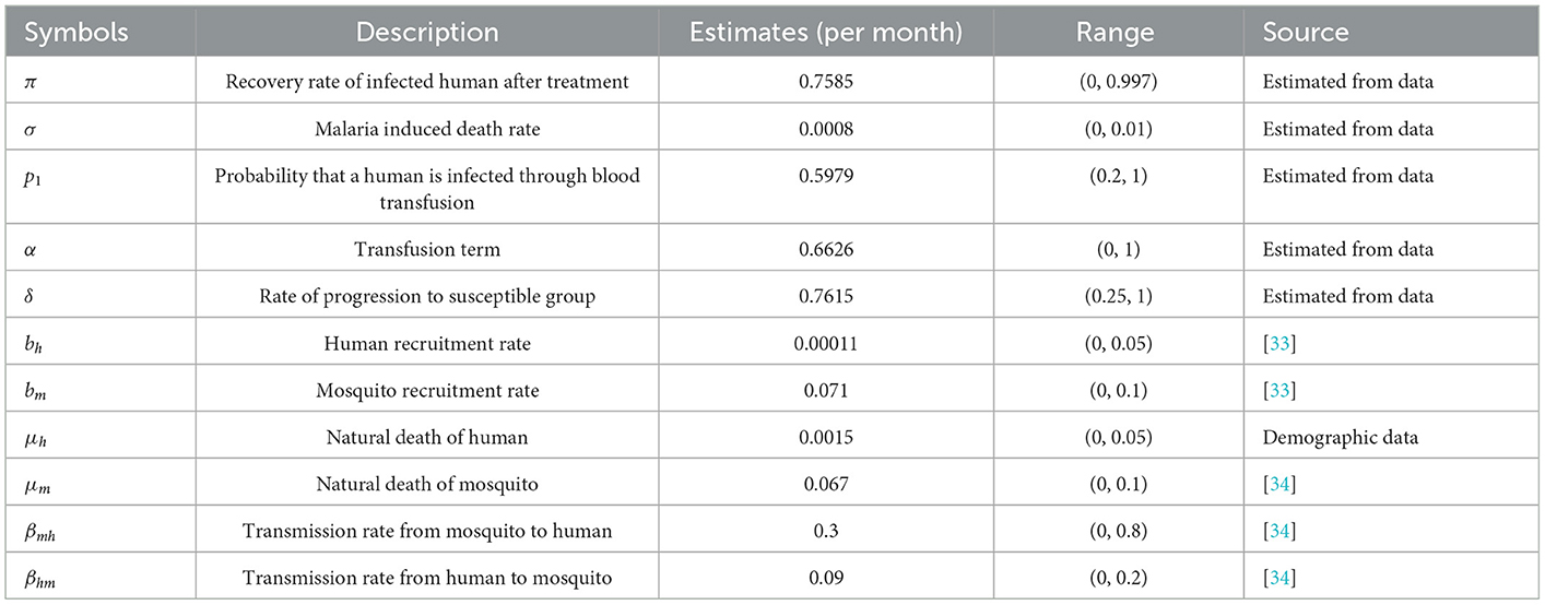
Table 1. Parameters and their estimates.

Where μ₀ = 55.12 is the average life expectancy of Nigeria at the time the data was collected. Note that μ_h was calibrated to a monthly rate. Thus the value of μ₀ is 0.0015, which implies that the natural death rate is approximately 15 out of 10,000 persons monthly. In simple terms, on average 15 out of 10,000 people die every month naturally. Without loss of generality, we can denote S_h(t) by just S_ht and the same for other variables. The recovery rate of infected humans after treatment, π is estimated by

$\begin{array}{ll}\widehat{\pi }=\frac{{\sum }_{t=1}^n{R}_{ht}}{{\sum }_{t=1}^n{I}_{ht}},& (5.27)\end{array}$

Where t, t = 1, 2, ..., n is time measured in months and n is the number of months covered. The variables R_ht and I_ht are the number of recovered humans and the number of infected humans at time t respectively.

Malaria induced death rate of infected humans, σ is estimated by

$\begin{array}{ll}\widehat{\sigma }=\frac{{\sum }_{t=1}^n{D}_{ht}}{{\sum }_{t=1}^n{I}_{ht}}.& (5.28)\end{array}$

The variable D_ht is the number of malaria induced deaths at time t. The probability that a human is infected through blood transfusion, p₁ is given by

$\begin{array}{ll}{\widehat{p}}_1=\frac{{\sum }_{t=1}^n{I}_{ht}}{{\sum }_{t=1}^n{E}_{ht}},& (5.29)\end{array}$

Where E_ht is the number of exposed humans to malaria through exposure to an infected mosquito bite or via infected blood transfusion. The transfusion rate, α is given by

$\begin{array}{ll}\widehat{\alpha }=\frac{{\sum }_{t=1}^n{I}_{ht}}{{\sum }_{t=1}^n{T}_{ht}},& (5.30)\end{array}$

Where T_ht number of humans whose blood was tested and screened for malaria. Based on Equations (5.29), (5.30), it should be noted that E(t) > T(t) for all t, so that α > p₁. This is enforced because the blood transfusion rate should be greater than the probability that a human is infected through blood transfusion. Recall from Equation (2.3) that

$\begin{array}{l}{S}_h^{\prime }=(1-p_1\alpha I_h)b_h-({\lambda }_h+{\mu }_h)S_h+\delta R_h,\hfill \end{array}$

at steady state, we have

$\begin{array}{l}0=(1-p_1\alpha I_h)b_h-({\lambda }_h+{\mu }_h)S_h+\delta R_h.\end{array}$

Solving for δ gives

$\begin{array}{ll}\widehat{\delta }=\frac{1}{n\bar{R}}\left[({\bar{\lambda }}_{ht}+{\mu }_h){\displaystyle \sum _{t=1}^n}{S}_{ht}-b_h+\alpha b_h{p}_1{\displaystyle \sum _{t=1}^n}{I}_{ht}\right],& (5.31)\end{array}$

Where $\widehat{\delta }$ is the estimate of the rate of progression to the susceptible group, δ; $\bar{R}$ is the period average for the number of recovered humans, and the term $\alpha b_h{p}_1\sum _{t=1}^n{I}_{ht}$ account for the force of infection as a result of blood transfusion, p₁ is the probability of effectively transfusing infected blood to a susceptible human, α is the transfusion term, b_h is the recruit rate of humans, and ${\bar{\lambda }}_{ht}$ is the average force of transmitting malaria infection from an infected mosquito-to-human, and it is given in Equation (2.1).

6. Statistical data analysis

6.1. Exploratory data analysis

The data analyzed is a time series of secondary data on the monthly incident of malaria in Benue State collected from the Benue State Ministry of Health from June 2013 to September 2016, spanning 40 months of data points. All the values of the variables are monthly and the parameters estimated are per month. Figures 4–7 are plotted in this study directly based on the Benue State malaria available data.

FIGURE 4

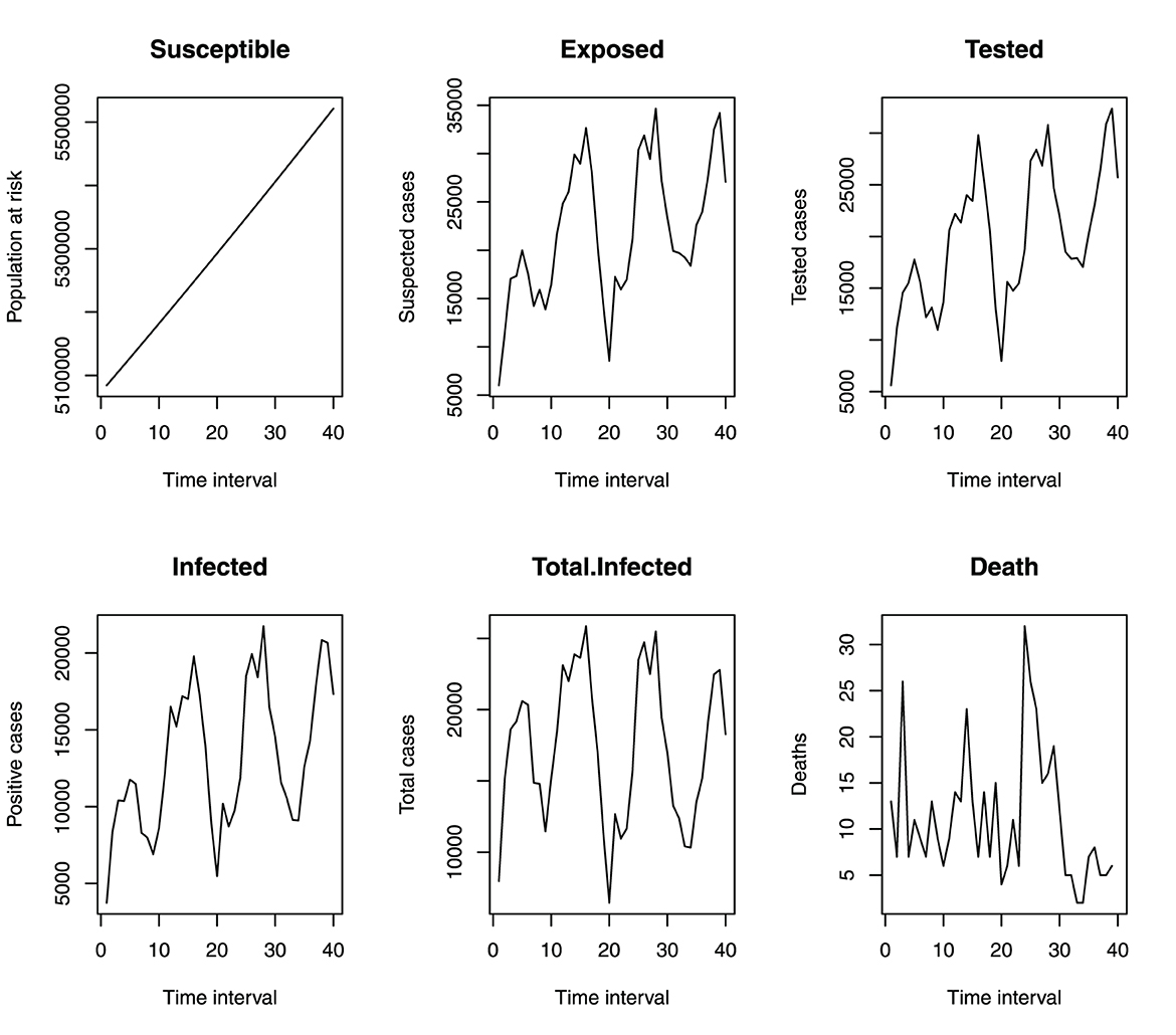
Figure 4. Monthly incident of malaria in benue.

Figure 4 shows that the incidence of malaria in Benue State depicts a seasonal variation. The incidence of malaria is always high at a particular time of the year (June to October) and always low from December to March. This variation is seen over the 4 years under study. Figure 5 shows the cumulative incidence of malaria. All the variables do not show any sign of flattened curves, except for deaths.

FIGURE 5

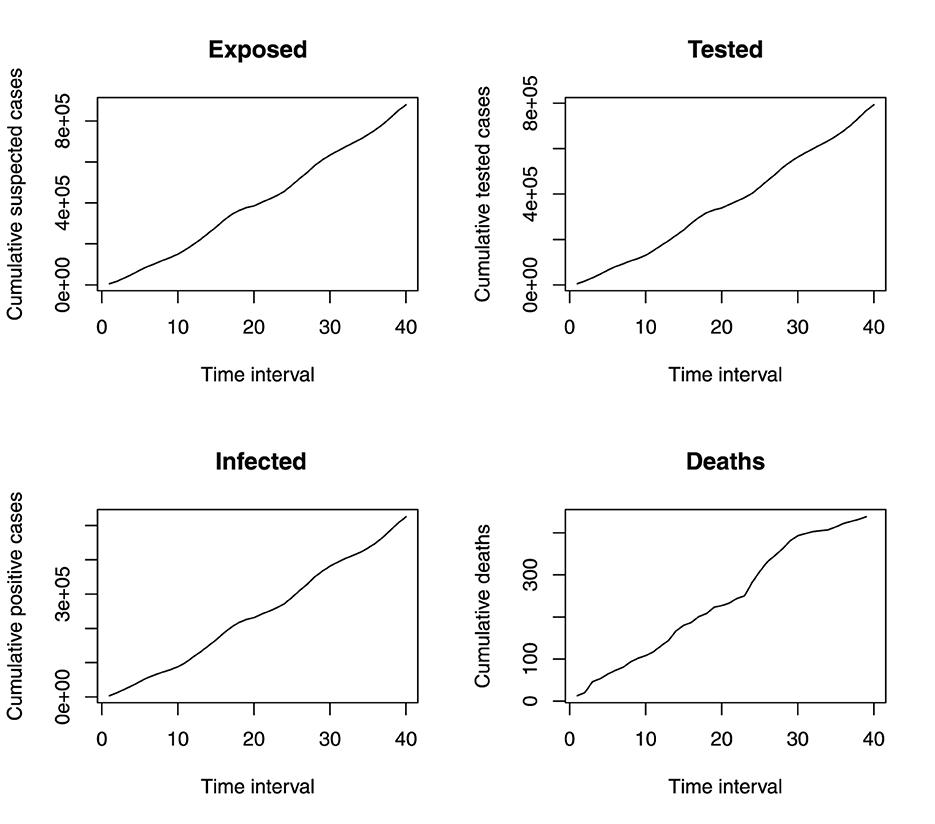
Figure 5. Monthly cumulative incident of malaria in benue.

Figure 6 depicts the distribution of monthly incidents of malaria in Benue State. The histograms show that the susceptible population is asymptotically uniformly distributed, the exposed population is negatively skewed, the tested population is approximately normally distributed, the infected and total infected have multiple local maximum points and death is positively skewed.

FIGURE 6

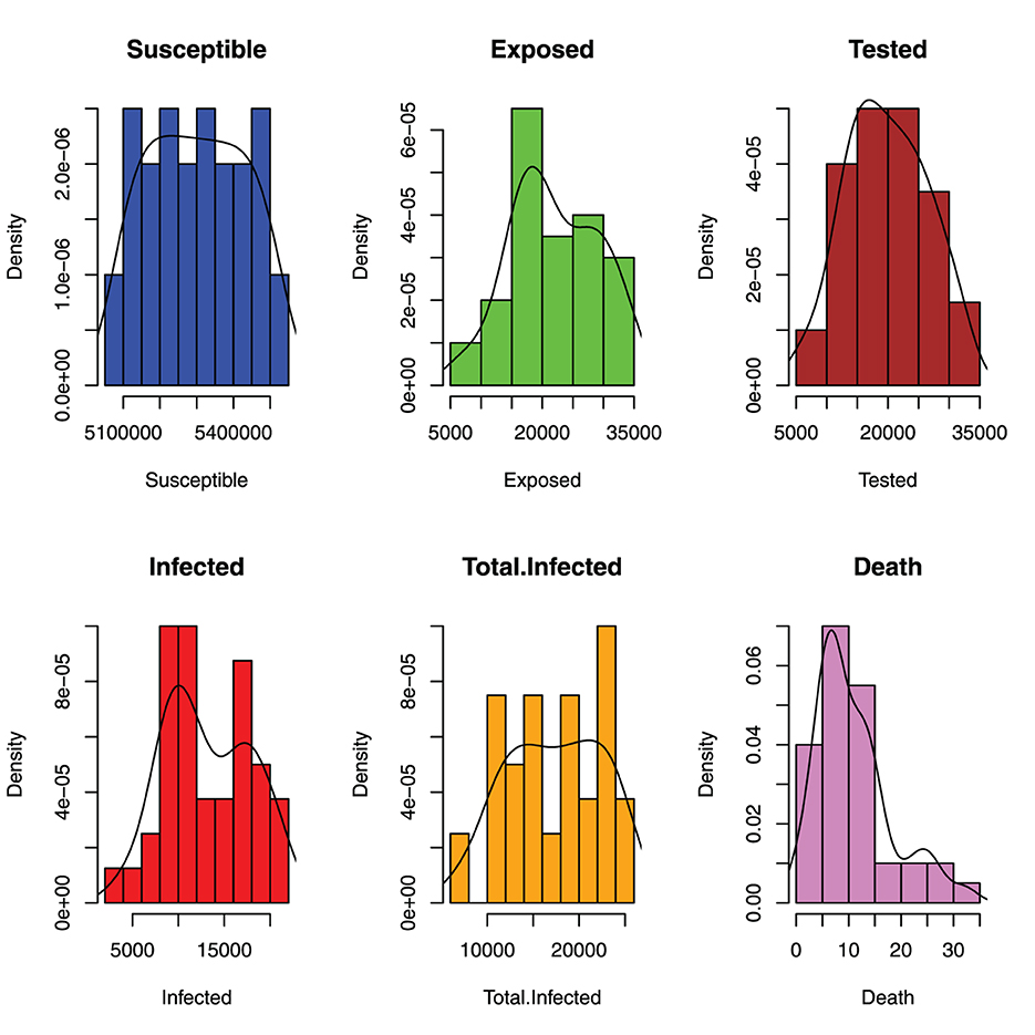
Figure 6. Distribution of monthly incident of malaria in benue.

Figure 7 shows the spread of the malaria incident in Benue State. The boxplots show that all the variables are highly spread as can be seen in the values of their standard deviations in Table 1.

FIGURE 7

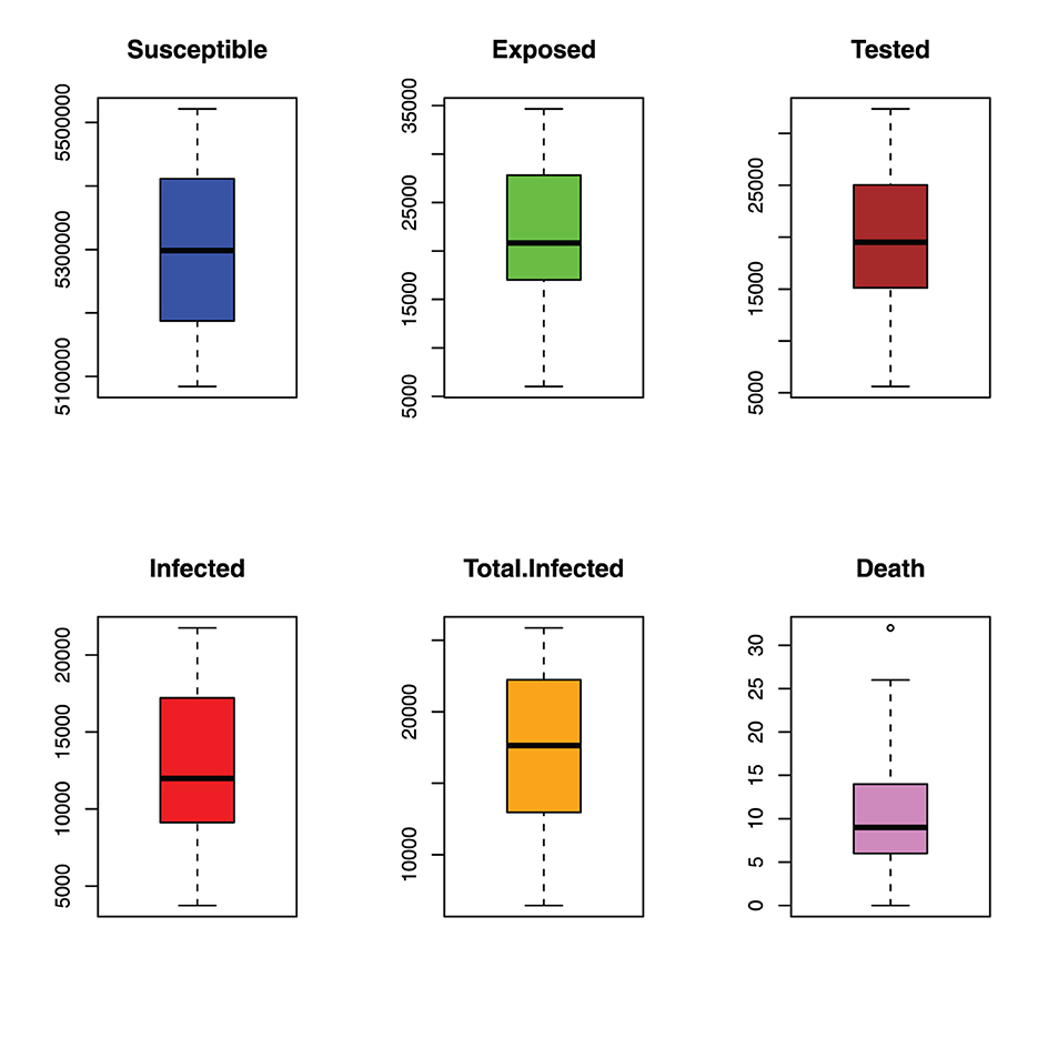
Figure 7. Spread of monthly incident of malaria in benue.

6.2. Variables predicted

Some of the variables used in the model are predicted using the parameters and the formulated models at a steady state. The ones where the data are available were not predicted and are shown in Table 1, but the ones whose real data are not available were predicted as displayed in Table 2. The results of the predicted variables are displayed in Table 3.

TABLE 2

Table 2. Predicted variables summary statistic.

TABLE 3

Table 3. Initial values of all variables of interest.

Table 1 shows the initial parameters used to fit the dynamic model. The initial values are the values in the initial month of the data collected. It should be noted that the data are monthly data.

6.3. Model fitting

The model fitting was performed using a genetic algorithm (GA) [35] for our function optimizer, using MATLAB; the GA helps us find the correct region of attraction, which provides the starting values for the parameters to be estimated in the fmincon function in the Optimization Toolbox of MATLAB. Hence, we shall be combining two optimization algorithms for our data fitting, a GA and the fmincon algorithm in MATLAB to get a more accurate estimate. Our model fitting is implemented for a malaria data set of Benue State, Nigeria from June 2013 to September 2016 (see Figure 8).

FIGURE 8

Figure 8. Model fitting using GA and the fmincon algorithm.

7. Numerical simulations and discussion of results

This section is devoted to numerically illustrating the theoretical results obtained in the model analysis. Table 1 present the parameter values and their sources. Where the parameter values are not available from literature or estimation, realistic values were assumed in the simulation. In the following, we simulate different combinations of treatment and preventive control measures to investigate their impact on malaria transmission. We have excluded simulating single controls following the recommendation of WHO [36] that a combination of controls is recommended to control/interrupt malaria transmission. Thus, we shall simulate to investigate the following scenarios:

(i) Possible combinations using two (2) controls only.

(ii) Possible combinations using three (3) controls only.

(iii) Possible combinations using four (4) controls only.

(iv) Possible combinations using all five (5) controls.

To perform the simulation, we assumed that the weight functions W_i, i = 1, 2, ..5, associated with the controls are unity. Also, the initial values for the state variables and parameter values are given in Tables 1, 3, respectively. The Supplementary Figures 7.1–7.26 represent the various scenarios described below can be seen on the Supplementary material. We next discuss the various scenarios arising from the simulations:

7.1. Optimal blood screening (u₁) and long lasting insecticide treated bednets (u₂)

Using this strategy, we optimize the objective function using the controls u₁ and u₂ when u₃ = u₄ = u₅ = 0, it can be seen from Supplementary Figure 7.1 that without the controls, there is a sharp decline in the number of susceptible humans that progresses to the infected humans. This is indeed the case as we have a high increase in the number of infected mosquitoes. In the presence of controls u₁ and u₂, susceptible humans maintained a constant level after about 50 months while the number of infected humans and infected vectors are reduced significantly after 50 months. It can also be observed from Supplementary Figure 7.1 that little or no humans are recovered.

7.2. Optimal blood screening (u₁) and treatment (u₃)

In this case, we simulated only u₁ and u₃ while other controls remain zero. Specifically, it can be noticed from Supplementary Figure 7.2 that the intervention strategies lead to a decrease in the number of both infected humans and mosquitoes as against an increase observed in the uncontrolled case, while at the same time, susceptible humans maintained a steady level and more humans recovered.

7.3. Optimal blood screening (u₁) and pesticide/chemicals spray (u₄)

Using this strategy, Supplementary Figure 7.3 shows that the adopted strategy does not have an impact on susceptible, infected, and recovered humans, respectively. It can also be observed from Supplementary Figure 7.3 that the combination of the controls u₁ and u₄ had little impact on the infected mosquito population, which explains why this strategy does not provide control on susceptible, infected and recovered humans.

7.4. Optimal blood screening (u₁) and indoor insecticide spray (u₅)

With this strategy, it was observed in Supplementary Figure 7.4 that there is a significant difference in I_h and I_m using controls u₁ and u₅ compared to I_h and I_m without control. This strategy also shows a significant difference in optimal Susceptible S_h compared to S_h in the uncontrolled case. Since there is no treatment strategy (u₃ = 0) in place, this strategy does not have control over recovered humans.

7.5. Optimal LLITBs (u₂) and treatment (u₃)

In Supplementary Figure 7.5, this strategy, when applied, shows a significant decrease in the number of infected humans and infected mosquitoes as against an increase observed in the uncontrolled case. Also, in the uncontrolled case, susceptible individuals stabilize for around 50 months while in the uncontrolled case, susceptible individuals are further depleted increasing the number of infected humans I_h. The strategy, also revealed that it is potent for recovered humans as shown in Supplementary Figure 7.5.

7.6. Optimal LLITBs (u₂) and pesticides/chemicals spray (u₄)

Here, the controls u₂ and u₄ are used to optimize the objective function with other controls u₁ = u₃ = u₅ = 0. The implementation of this strategy revealed in Supplementary Figure 7.6 that the number of infected humans and infected mosquitoes differs significantly from the uncontrolled case. The figure further showed that there is no significant impact on recovered individuals since treatment u₃ = 0 is not considered in this strategy. This strategy shows a close difference between controlled and uncontrolled susceptible humans.

7.7. Optimal LLITBs (u₂) and indoor insecticide spray (u₅)

In this scenario, the controls u₂ and u₅ are used to optimize the objective function, with other controls set to zero. Supplementary Figure 7.7 shows that this strategy has little effect on susceptible humans becoming infected. It can be seen that the number of susceptible humans in both controlled and uncontrolled cases is very close. This strategy also provides no control over the recovered humans. In Supplementary Figure 7.7, there is little difference in the number of infected humans between the controlled and uncontrolled cases. Further, the number of infected mosquitoes is reduced for the controlled case when compared to the uncontrolled case.

7.8. Optimal treatment (u₃) and pesticides/chemicals spray (u₄)

The objective function is optimized in this case by u₃ and u₄ while other controls u₁, u₂, and u₅ are set to zero. In Supplementary Figure 7.8, by using this strategy, there is a significant difference in the number of susceptible humans in the controlled case compared to the uncontrolled case. This strategy also shows that there is a significant difference in the number of infected mosquitoes compared to the uncontrolled case. Similarly, using this strategy, there is a sharp difference in the number of infected humans with fluctuations before finally settling down around 60 months. This account for the considerable difference in the number of recovered humans using this strategy. It is also observed in Supplementary Figure 7.8, the recovery of individuals occurs with oscillations before finally settling to a steady state around 60 months.

7.9. Optimal treatment (u₃) and indoor insecticide spray (u₅)

This strategy involves the optimization of the objective function using u₃ and u₅ while other controls are set to zero. In Supplementary Figure 7.9, it is shown that there is a significant difference in the number of susceptible individuals in the controlled case compared to the uncontrolled case. This strategy shows that it is effective for recovered humans as there are few or no individuals left to recover from the disease. The number of infected humans and infected mosquitoes is significantly reduced in the controlled case as against when there is no control.

7.10. Optimal pesticides/chemicals spray (u₄) and indoor insecticide spray (u₅)

The objective function is optimized using the controls u₄ and u₅ with u₁ = u₂ = u₃ = 0. The result of this strategy as shown in Supplementary Figure 7.10 revealed that it impact the reduction of infected mosquitoes significantly as compared to the uncontrolled case. With control, the number of infected individuals dropped significantly to about 500, 000 infected individuals as against 2Million infected individuals in the uncontrolled case. However, this strategy does not have any impact on recovered individuals. The simulation in Supplementary Figure 7.10, revealed that in the uncontrolled case, more susceptible humans progress significantly to the infected class when compared to the controlled case.

7.11. Optimal blood screening (u₁), LLITBs u₂ and treatment (u₃)

The combination of the controls u₁, u₂, and u₃ are used to optimize the objective function while keeping u₄ and u₅ to be zero. Using this intervention strategy, it can be seen in Supplementary Figure 7.11, for the controlled case, the number of infected humans and infected mosquitoes is reduced significantly while a considerable increase is observed when control is not in place. It can be seen in Supplementary Figure 7.11, that for the strategy, the recovered class display oscillations which may suggest that disease transmission may increase/decrease during certain months of the year. With control in place, the number of susceptible individuals is maintained at a steady level as against the sharp decline in the number of susceptible when there is no control.

7.12. Optimal blood screening (u₁), LLITBs u₂ and pesticide/chemical spray (u₄)

The objective function is optimized using the controls u₁, u₂, and u₄ with u₃ = 0 and u₅ = 0 is not effective to aid human recovery from the disease, however, a significant decrease is observed in the number of infected humans and infected mosquitoes when this strategy is implemented as compared when there is no control. This strategy can keep the number of susceptible humans at a steady level while the number decreases significantly when there is no control in place.

7.13. Optimal blood screening (u₁), LLITBs u₂ and indoor insecticide spray (u₅)

The controls u₁, u₂ and u₅ are used to optimize the objective function while setting u₃ and u₄ to zero. From Supplementary Figure 7.13, it can be seen that there is little difference in the number of susceptible individuals between the controlled and uncontrolled cases, while the strategy does not affect number of recovered humans. There is little difference in the number of infected humans with control and when control is not in place. With control, it is observed in Supplementary Figure 7.3 that the number of infected mosquitoes is reduced by half while the number of infected mosquitoes is doubled in the absence of controls.

7.14. Optimal blood screening (u₁), treatment u₃, and pesticides/chemicals spray (u₄)

The objective function in this case is optimized using u₁, u₃ and u₄ with u₂ = 0 and u₅ = 0. Supplementary Figure 7.14, shows that the strategy has significant control on susceptible humans and infected mosquitoes, respectively. It can also be seen that the control has a significant effect on the number of infected humans and recovered humans, respectively. The oscillations observed in the controlled cases for both infected and recovered humans may be a result of the varying transmission of the disease during certain months of the year.

7.15. Optimal blood screening (u₁), treatment u₃, and indoor insecticide spray (u₅)

In this instance, only the controls u₁, u₃ and u₅ are used to optimize the objective function. In Supplementary Figure 7.15, the strategy shows that the number of susceptible and recovered humans is increased compared to the uncontrolled case. It is also observed using this strategy, decreases the number of infected humans and vectors for the controlled case as against the increase observed when there is no control.

7.16. Optimal blood screening (u₁), pesticides/chemicals u₄ spray, and indoor insecticide spray (u₅)

The objective function is optimized using combination of controls u1, u4, and u5 with u2 = u3 = 0. As shown in Supplementary Figure 7.16, the strategy has little impact on susceptible humans while it has no impact on recovered humans. It can be seen in Supplementary Figure 7.16, that the strategy has an impact in reducing the number of infected mosquitoes as against the uncontrolled case. The number of infected humans in the controlled case is about half of the uncontrolled case.

7.17. Optimal LLITBs (u₂), treatment u₃, and pesticides/chemicals spray (u₄)

This strategy optimizes the objective function using the combination of the controls u2, u3, and u4. In Supplementary Figure 7.17, this strategy has a significant impact in controlling the number of susceptible humans, infected humans, recovered humans, and infected mosquitoes compared to the uncontrolled case.

7.18. Optimal LLITBs (u₂), treatment u₃, and indoor insecticide spray (u₅)

The combination of the controls (u₂), (u₃), and (u₅) with (u₁ = u₄ = 0) are used to optimize the objective function in this instance. From Supplementary Figure 7.18, this strategy has a significant impact on controlling malaria disease. Using this strategy, the number of infected humans and mosquitoes is significantly reduced with more individuals recovering from the disease after treatment. In the controlled case, the progression of susceptible humans is significantly reduced compared to the uncontrolled case.

7.19. Optimal LLITBs (u₂), treatment (u₃), and indoor insecticide spray (u₅)

The objective function in this case is optimized using controls (u₂), (u₄), and (u₅) when u₁ and u₃ are zero. The simulation using this strategy revealed that it has very little impact in controlling malaria disease transmission. Specifically, it can be seen in Supplementary Figure 7.19 that the number of infected humans and mosquitoes is still high despite the control with no humans recovered. It can be observed that only a few susceptible humans are protected from getting infected as there is little difference between the controlled and uncontrolled cases for susceptible humans.

7.20. Optimal treatment (u₃), pesticide/chemicals spray (u₄), and indoor insecticide spray (u₅)

We optimize the objective function using the combination of the controls u₃, u₄ and u₅ with u₁ and u₂ assumed to be zero. The simulation result in Supplementary Figure 7.20 shows that this strategy is highly effective in controlling malaria disease transmission. With this strategy in place, it can be seen in Supplementary Figure 7.20 that the number of infected humans and mosquitoes is significantly reduced while a significant number of humans recovered from the disease. The simulation also indicates that more individuals are less susceptible to malaria as a result of this strategy.

7.21. Optimal blood screening (u₁), LLITBs (u₂), treatment (u₃), and pesticide/chemicals spray (u₄)

The objective function is optimized using the controls u₁, u₂, (u₃), and u₄ with u₅ = 0. We observe from Supplementary Figure 7.21 that the number of recovered humans and susceptible individuals differ considerably compared to when there is no control. Furthermore, Supplementary Figure 7.21, reveals that the number of infected humans and infected mosquitoes is lower when compared with the case without control.

7.22. Optimal blood screening (u₁), LLITBs (u₂), treatment (u₃), and indoor insecticide spray (u₅)

With this strategy, the controls u₁, u₂, (u₃), and u₅ are used to optimize the objective function with u₄ = 0. For this strategy, shown in Supplementary Figure 7.22, we observe a significant difference in the number of susceptible humans, infected humans, recovered humans, and infected mosquitoes with optimal strategy compared to susceptible humans, infected humans, recovered humans, and infected mosquitoes without control.

7.23. Optimal LLITBs (u₂), treatment (u₃), pesticide/chemicals spray ((u₄), and indoor insecticide spray (u₅)

With this strategy, the objective function is optimized using the combination of the controls u₂, (u₃),((u₄), and u₅ while setting u₁ to zero. Observe from Supplementary Figure 7.23 that this optimal strategy shows a significant difference in the number of susceptible individuals, infected humans, and infected mosquitoes as against the uncontrolled case.

7.24. Optimal blood screening (u₁), LLITBs (u₂), treatment (u₃), pesticide/chemicals spray ((u₄), and indoor insecticide spray (u₅)

In this case, all the five controls u₁, u₂, u₃,u₄, and u₅ are used to optimize the objective function. With this strategy, it is observed in Supplementary Figure 7.24 that the control strategies resulted in a significant decrease in the number of infected humans and mosquitoes as against an increase in the number of infected humans and mosquitoes when no control is applied. Similarly, there is an increase in the number of recovered humans when controls are in place compared to the decrease in the number of required humans in the absence of no control. With optimal strategy, the number of susceptible humans differs considerably compared to the uncontrolled case.

In Supplementary Figures 7.25, 7.26, the control profiles are displayed. In Supplementary Figure 7.25, the control profile using blood screening, u₁ became about 20% effective after 130months which was soon increased to around 39% effective in another 45 months before declining. The control u₂, became about 15% effective for over 150months before declining. For the first 170 months, u₃ was 15% effective before experiencing a sharp decline for about 20 months and thereafter picked up again. About 40% effectiveness was achieved in the control of malaria using control u₄ and u₅ before steadily declining after 60 months and 90 months, respectively. In Supplementary Figure 7.26, the profiles for all the control are presented. It can be seen that controls u₄ and u₅ perform optimally, this is closely followed by u₁ while both u₂ and u₃ are next.

From the foregoing discussion, it can be seen from our simulations that the combination of using all the five (5) controls (u₁, u₂, u₃, u₄, u₅), the combination of four (4) controls [(u₁, u₂, u₃, u₅) and (u₂, u₃, u₄, u₅)], and combination of three (3) controls [(u₂, u₃, u₅) and (u₃, u₄, u₅)] have the highest impact on malaria disease control. A further look into the suggested combinations shows that controls u₂, u₃ and u₅ are common to all the combinations, that is the combination (u₂, u₃, u₄, u₅)) where resources are scarce may be sufficient to control the spread of malaria.

The above scenarios of the controls can be best interpreted to mean that for malaria disease eradication, more combinations of the controls are suggested depending on the area and availability of resources. This submission is in line with World Health Organization's (WHO) position that only one control strategy is not sufficient to interrupt malaria transmission [36].

8. Conclusion

A mathematical analysis of the blood transfusion-transmission dynamics of malaria disease has been rigorously studied in this work. The malaria model under investigation revealed that there exists a relationship between the reproduction number for malaria (R₀) and the reproduction number for malaria induced through blood transfusion R_α. The study further revealed that the basic reproduction number is sensitive to parameters such as the transmission rate from mosquito-to-humans β_mh, transmission rate from humans-to-mosquito β_hm blood transfusion reproduction number R_α, recruitment rate of the mosquitoes b_m. The malaria disease-free equilibrium, M₀ is locally globally asymptotically stable if both R₀ and R_α are less than or equal to unity. The implicit function theorem was used to investigate the local stability of the malaria endemic equilibrium M^⋆. The result revealed that M^⋆ may undergo a supercritical (forward) bifurcation if the quantity $\frac{A}{B}<1$ or a subcritical (backward) bifurcation if the quantity $\frac{A}{B}>1$. Consequently, an optimal control problem using both time-dependent preventive and treatment controls to mitigate the disease was studied using the Pontryagins Maximum Principle. The results revealed that the combination of all the five (5) controls (u₁, u₂, u₃, u₄, u₅), combination of four (4) controls [(u₁, u₂, u₃, u₅) and (u₂, u₃, u₄, u₅)], and combination of three (3) controls [(u₂, u₃, u₅] and u₃, u₄, u₅)] are recommended to mitigate against malaria transmission. In areas where resources are scarce, our study revealed that using the combination of u₂, u₃, and u₅ is sufficient to effectively interrupt the transmission of malaria disease. Indeed, our results also agree with earlier studies in Blayneh et al. [14] and Agusto et al. [13] on malaria control, however, our results present five possible control strategies that are sufficient to minimize the transmission of malaria. Subsequently, exploratory data analysis (EDA) was performed on the malaria data from Benue State Nigeria. The model was fitted to data and it can be seen that our model gave a good fit.

In conclusion, the present study has provided us with a mathematical understanding of malaria dynamics taking into account transmission via blood transfusion and mosquitoes. As a suggestion for future research, it will be of interest to study the cost-effectiveness analysis of the controls studied in this work.

Data availability statement

The raw data supporting the conclusions of this article will be made available by the authors, without undue reservation.

Author contributions

MA: conceptualization and writing original draft. OA: formal analysis. OO: literature review. ME: analysis and parameter estimation. MM: data curation and validation. SO: review and editing. DN: visualization. All authors contributed to the article and approved the submitted version.

Conflict of interest

The authors declare that the research was conducted in the absence of any commercial or financial relationships that could be construed as a potential conflict of interest.

Publisher's note

All claims expressed in this article are solely those of the authors and do not necessarily represent those of their affiliated organizations, or those of the publisher, the editors and the reviewers. Any product that may be evaluated in this article, or claim that may be made by its manufacturer, is not guaranteed or endorsed by the publisher.

Supplementary material

The Supplementary Material for this article can be found online at: https://www.frontiersin.org/articles/10.3389/fams.2023.1105543/full#supplementary-material

References

1. Owusu O, Alex K, Christopher P. Transmitted malaria in countries where malaria is endemic: a review of the literature from Sub-Saharan Africa. SAGE Open Med. (2010) 51:1192–8. doi: 10.1086/656806

PubMed Abstract | CrossRef Full Text | Google Scholar

2. World Health Organization. Screening Donated Blood for Transfusion-Transmissible Infections. (2010).

Google Scholar

3. Mohammed Y, Bekele A. Seroprevalence of transfusion transmitted infection among blood donors at Jijiga blood bank, Eastern Ethiopia. BMC Res Notes. (2016) 9:1199–200. doi: 10.1186/s13104-016-1925-6

PubMed Abstract | CrossRef Full Text | Google Scholar

4. Bhat S, Desai AS. Effectiveness of multimodal ayurvedic treatment in Vataja Pandu wsr nutritional deficiency anemia-a case report. Int J Ayurveda Pharma Res. (2022) 10:32–9. doi: 10.47070/ijapr.v10i1.1617

CrossRef Full Text | Google Scholar

5. Kitchen A, Seed R, Davis T. The current status and poten-tial role of laboratory testing to prevent transfusion-transmit-ted malaria. Transfus Med Rev. (2005) 1:229–40. doi: 10.1016/j.tmrv.2005.02.004

PubMed Abstract | CrossRef Full Text | Google Scholar

6. World Health Organization. National Standards for Blood Transfusion Service. Thimphu: Ministry of Health (2013).

7. Kitchen D, Chiodini L. Malaria and blood transfusion. VoxSang. (2006) 1:77–84. doi: 10.1111/j.1423-0410.2006.00733.x

PubMed Abstract | CrossRef Full Text | Google Scholar

8. Hirigo AT, Abiy Z, Tsehay S, Hassen F, Desta K. Blood transfusion-transmissible malaria and its cost analysis in Hawassa regional blood bank, Southern Ethiopia. SAGE Open Med. (2020) 8:1–9. doi: 10.1177/2050312120936930

PubMed Abstract | CrossRef Full Text | Google Scholar

9. Bruce C. Transfusion malaria revisited (1982).

Google Scholar

10. Olaniyi S, Obabiyi O. Mathematical model for malaria transmission dynamics in human and mosquito populations with nonlinear forces of infection. Int J Pure Appl Math. (2013) 88:125–56. doi: 10.12732/ijpam.v88i1.10

CrossRef Full Text | Google Scholar

11. Reesink H. European strategies against the parasite transfusion risk. Transfus Clin Biol. (2005) 12:1–4. doi: 10.1016/j.tracli.2004.12.001

PubMed Abstract | CrossRef Full Text | Google Scholar

12. Reesink H, Panzer S, Wendel S, Levi J, Ullum H, Ekblom-Kullberg S, et al. The use of malaria antibody tests in the prevention of transfusion-transmitted malaria. Vox Sanguinis. (2010) 98:468–78. doi: 10.1111/j.1423-0410.2009.01301.x

PubMed Abstract | CrossRef Full Text | Google Scholar

13. Agusto FB, Marcus N, Okosun KO. Application of optimal control to the epidemiology of malaria (2012).

Google Scholar

14. Blayneh K, Cao Y, Kwon HD. Optimal control of vector-borne diseases: treatment and prevention. Discrete Contin Dyn Syst B. (2009) 11:587. doi: 10.3934/dcdsb.2009.11.587

CrossRef Full Text | Google Scholar

15. Adeniyi MO, Aderele OR. Mathematical analysis of transfusion–transmitted malaria model with optimal control. Preprints. (2019) 2018:2018090214. doi: 10.20944/preprints201809.0214.v2

CrossRef Full Text

16. Zhao R, Liu Q. Dynamical behavior and optimal control of a vector-borne diseases model on bipartite networks. Appl Math Model. (2022) 102:540–63. doi: 10.1016/j.apm.2021.10.011

CrossRef Full Text | Google Scholar

17. Abboubakar H, Guidzavaï AK, Yangla J, Damakoa I, Mouangue R. Mathematical modeling and projections of a vector-borne disease with optimal control strategies: Aacase study of the Chikungunya in Chad. Chaos Solitons Fractals. (2021) 150:111197. doi: 10.1016/j.chaos.2021.111197

CrossRef Full Text | Google Scholar

18. Oluyo TO, Adeniyi MO. The mathematical analysis of malaria transmission: the effect of sanitation. Int J Sci Res. (2018) 7:236–44.

Google Scholar

19. Oluyo TO, Adeniyi MO. Mathematical analysis of malaria-pneumonia model with mass action. Int J Appl Math. (2014) 29:1333.

Google Scholar

20. Oke SI, Ojo MM, Adeniyi MO, Matadi MB. Mathematical modeling of malaria disease with control strategy. Commun Math Biol Neurosci. (2020) 2020:43. doi: 10.28919/cmbn/4513

CrossRef Full Text | Google Scholar

21. Diekmann O, Heesterbeek JAP, Metz JA. On the definition and the computation of the basic reproduction ratio R 0 in models for infectious diseases in heterogeneous populations. J Math Biol. (1990) 28:365–82. doi: 10.1007/BF00178324

PubMed Abstract | CrossRef Full Text | Google Scholar

22. Van den Driessche P, Watmough J. Reproduction numbers and sub-threshold endemic equilibria for compartmental models of disease transmission. Math Biosci. (2002) 180:29–48. doi: 10.1016/S0025-5564(02)00108-6

PubMed Abstract | CrossRef Full Text | Google Scholar

23. Adeniyi MO, Oke SI, Ekum MI, Benson T, Adewole MO. Assessing the impact of public compliance on the use of non-pharmaceutical intervention with cost-effectiveness analysis on the transmission dynamics of COVID-19: insight from mathematical modeling. In: Modeling, control and Drug Development for COVID-19 Outbreak Prevention. Springer (2022). p. 579–618.

Google Scholar

24. Adeniyi MO, Ekum MI, Iluno C, Oke SI. Dynamic model of COVID-19 disease with exploratory data analysis. Sci Afr. (2020) 9:e00477. doi: 10.1016/j.sciaf.2020.e00477

PubMed Abstract | CrossRef Full Text | Google Scholar

25. Chukwu A, Akinyemi J, Adeniyi M, Salawu S. On the reproduction number and the optimal control of infectious diseases in a heterogenous population. Adv Diff Equat. (2020) 2020:1–14. doi: 10.1186/s13662-020-03050-9

CrossRef Full Text | Google Scholar

26. Buonomo B, Lacitignola D. On the backward bifurcation of a vaccination model with nonlinear incidence. Nonlinear Anal Model Control. (2011) 16:30–46. doi: 10.15388/NA.16.1.14113

PubMed Abstract | CrossRef Full Text | Google Scholar

27. DeJesus EX, Kaufman C. Routh-Hurwitz criterion in the examination of eigenvalues of a system of nonlinear ordinary differential equations. Phys Rev A. (1987) 35:5288. doi: 10.1103/PhysRevA.35.5288

PubMed Abstract | CrossRef Full Text | Google Scholar

28. Zhou P, Hu X, Zhu Z, Ma J. What is the most suitable Lyapunov function? Chaos Solitons Fractals. (2021) 150:111154. doi: 10.1016/j.chaos.2021.111154

CrossRef Full Text | Google Scholar

29. Boldin B. Introducing a population into a steady community: the critical case, the center manifold, and the direction of bifurcation. SIAM J Appl Math. (2006) 66:1424–53. doi: 10.1137/050629082

CrossRef Full Text | Google Scholar

30. Pontryagin LS. Mathematical Theory of Optimal Processes. London: Routledge (2018).

Google Scholar

31. Fleming WH, Rishel RW. Deterministic and Stochastic Optimal Control. Vol. 1. Springer Science & Business Media (2012).

Google Scholar

32. Abidemi A, Olaniyi S, Adepoju OA. An explicit note on the existence theorem of optimal control problem. J Phys.(2022) 2199:012021. doi: 10.1088/1742-6596/2199/1/012021

CrossRef Full Text | Google Scholar

33. Agusto FB, Tchuenche JM. Control strategies for the spread of malaria in humans with variable attractiveness. Math Populat Stud. (2013) 20:82–100. doi: 10.1080/08898480.2013.777239

CrossRef Full Text | Google Scholar

34. Olaniyi S, Okosun K, Adesanya S, Lebelo R. Modelling malaria dynamics with partial immunity and protected travellers: optimal control and cost-effectiveness analysis. J Biol Dyn. (2020) 14:90–115. doi: 10.1080/17513758.2020.1722265

PubMed Abstract | CrossRef Full Text | Google Scholar

35. McCall J. Genetic algorithms for modelling and optimisation. J Comput Appl Math. (2005) 184:205–22. doi: 10.1016/j.cam.2004.07.034

CrossRef Full Text | Google Scholar

36. Aregawi M, Cibulskis RE, Otten M, Williams R. World Malaria Report 2009. World Health Organization (2009).

Google Scholar