 Yuanming Lu
 Junfei Xia2
 Lukas J. Magee
 Donald L. DeAngelis
94% of researchers rate our articles as excellent or good
Learn more about the work of our research integrity team to safeguard the quality of each article we publish.
Find out more
ORIGINAL RESEARCH article
Front. Appl. Math. Stat., 23 March 2023
Sec. Mathematical Biology
Volume 9 - 2023 | https://doi.org/10.3389/fams.2023.1086781
This article is part of the Research TopicDo individuals matter? - Individual-based versus population-based models applied to biology and healthView all 5 articles
Invasive plant species alter community dynamics and ecosystem properties, potentially leading to regime shifts. Here, the invasion of a non-native tree species into a stand of native tree species is simulated using an agent-based model. The model describes an invasive tree with fast growth and high seed production that produces litter with a suppressive effect on native seedlings, based loosely on Melaleuca quinquenervia, invasive to southern Florida. The effect of a biocontrol agent, which reduces the invasive tree's growth and reproductive rates, is included to study how effective biocontrol is in facilitating the recovery of native trees. Even under biocontrol, the invader has some advantages over native tree species, such as the ability to tolerate higher stem densities than the invaded species and its litter's seedling suppression effect. We also include a standing dead component of both species, where light interception from dead canopy trees influences neighboring tree demographics. The model is applied to two questions. The first is how the mean seedling dispersal rate affects the spread of the invading species into a pure stand of natives, assuming the same mean dispersal distance for both species. For assumed litter seedling suppression that roughly balances the fitness levels of the two species, which species dominates depends on the mean dispersal distance. The invader dominates at both very high and very low mean seedling dispersal distances, while the native tree dominates for dispersal distances in the intermediate range. The second question is how standing dead trees affect either the rate of spread of the invader or the rate of recovery of the native species. The legacy of standing dead invasive trees may delay the recovery of native vegetation. The results here are novel and show that agent-based modeling is essential in illustrating how the fine-scale modeling of local interactions of trees leads to effects at the population level.
Modeling of species invasions goes back to at least the study conducted by Skellam [1], who used random-walk and reaction-diffusion modeling to describe the spread of oaks in Europe following the last Ice Age and the more recent invasion of a small invasive mammal, the muskrat. The use of reaction-diffusion models to describe invasions has been applied over the decades and has been useful in predicting key aspects of invasions, such as the speed of spread and mean width of a wavefront, in terms of population growth rate and dispersal coefficient [e.g., [2, 3]]. Taking into account that the invasion process is far more complex than simple reaction-diffusion equations, mathematical modelers have made numerous extensions to describe more details of populations and their environments, such as the Allee effect, population stage structure, and environmental heterogeneity [4].
However, the recent history of ecology of invasions has been toward the inclusion of factors that are less amenable to purely mathematical approaches but are easily included in spatially explicit individual- or agent-based modeling (we will use the latter term, or ABM for short). These factors include variability among population members, high spatial heterogeneity, microscale interactions, and demographic stochasticity. The importance of such factors has been recognized as relevant to understanding plant community dynamics in general. To explain the long-term coexistence of many species in tree communities, Clark [5] and Clark et al. [6] asserted that it is necessary to look at the competition at the level of individual trees, noting that competition is local, between individuals, and that calculation of competition coefficients at the level of species tends to wash out these individual-level effects; note though, there has been disagreement on whether individual-level competition can facilitate coexistence [7]. This, as well as other important features of individuals, such as the growth of juveniles into the adult stage and survival of adults, has been incorporated into ABM models and tested [8], as has spatial heterogeneity in the model of Goslee et al. [9]. A growing body of spatially explicit ABM models now exists. As stressed by some authors of ABMs for invasion ecology, it is important as much as possible to compare ABMs with mathematical models or, better, use them in combination [10, 11].
Invasion of a new plant species into a community involves both competition at the local level and movement in space, and a spatially explicit ABM model is well-equipped to describe such dynamics. Our objective here is to show that spatially explicit ABMs can be used to reveal phenomena involving invasive populations and native populations, particularly at the interface of their encounter. Our model was originally developed for a tree species invasion in southern Florida [12]. As in many other locales globally, a variety of invasions have occurred and are occurring in southern Florida habitats. Some are cases of native species invading other native species, such as mangroves into hardwood hammocks [e.g., [13]] or mangroves into salt marshes [14]. Those invasions result from temporal changes in sea level and minimum winter temperatures, respectively, which change the environmental gradient, allowing one species to expand its spatial range at the expense of the other. While range expansion of native species such as mangroves threatens important habitats, such as hardwood hammocks, the most damage economically and to native communities has been from alien species, such as Melaleuca quinquenervia, which we will refer to as simply Melaleuca. The expansion of Melaleuca into various native habitats of Florida has not involved climatic change, but simply superior competitive ability over native species, largely resulting from a lack of natural enemies in the invaded environment. Currently, biocontrol agents introduced from Melaleuca's native Australia are being used, including an introduced weevil, Oxyops vitos, to reduce the growth and reproductive potential of Melaleuca [12]. Their success in doing so is evidence of the relative lack of effective natural enemies of Melaleuca that are native to southern Florida. The decrease in Melaleuca's reproductive rate and in the tree's growth, and thus increase in mortality rate, shows signs of allowing existing native vegetation to gain a sufficient advantage to reverse the invasion, although the time scale of the introduction of biocontrol has been too short to gauge long-term trends. The effect of biocontrol on Melaleuca has substantially lowered its rate of seedling production. However, Melaleuca has advantages that may slow the recovery of native vegetation in areas that it covers. Melaleuca produces a large amount of litter that is slower to decompose than that of native vegetation. Rayamajhi et al. [15] demonstrated that its litter could suppress the emergence of native seedlings, in particular, two species common in southern Florida, wax myrtle (Morella cerifera) and sawgrass (Cladium jamaicense). The authors found that its litter had a greater suppressive effect on the emergence of the seedlings of the two native species than on its own seedlings. The suppressive effect of Melaleuca litter on seedlings may be a factor in its success as an invader. It is important to study the impact of the negative effect of litter on the emergence of seedlings, as has been observed in a number of studies of other competitive interactions of plants, including in plant invasions. A review by Xiong and Nilsson [16] of data from 35 independent studies on plant litter showed variable, but mostly negative, effects of litter on the germination and establishment of plants. That negative effect in turn has been shown to have effects at the community level [e.g., [17, 18]].
Although the biocontrol of Melaleuca lowers its competitive ability, making conditions more favorable for the recovery of native vegetation, the effect of Melaleuca's litter suppressing native seedings may slow the dynamics of recovery. Therefore, we model a two-species competition loosely based on the competition of the invasive Melaleuca with a generic native tree species. Our model, called ManHam, is based on an approximate parameterization of the life cycle of Melaleuca trees and of hardwood hammocks, the proxy tree species used to represent one of the native habitats that Melaleuca has invaded. Our simulations will show the parameter ranges over which one or the other population can spread at the expense of the other. Holt et al. [19] speculated that cases may also exist where a wave of invaders is held stationary by native species along a boundary zone. We believe that there may be an interaction between litter suppression of seedlings by the invasive species and the mean dispersal distance of seeds that leads to one or the other of these possibilities in the presence of biocontrol. Therefore, one focus of our simulations here is to study the effects of different values for the effective mean distance of seedling establishment from the parent.
A second focus of our study is to include the effects of standing dead trees on the competition outcome. Invasion and biocontrol implementation will produce many dead trees (i.e., snags) that may remain standing for several years post-mortality [20]. Species interactions in forest ABMs rarely consider the residual effects of dead trees. Persistent root bases prevent seedling establishment and vegetation encroachment, residual light interception from dead canopies can deplete available light [21], and short-lived legacies of plant-soil feedbacks may also influence current regeneration dynamics [22–24].
The rates of decay and fall of standing dead trees can have substantial impacts on the regeneration environment [25] but have not, to the best of our knowledge, been included in models of forest dynamics. In the context of Melaleuca, persistent negative interactions post-mortality may inhibit the recovery of native trees. As native tree seedlings attempt to capitalize on resource pulses and replace dead canopy trees, slight residual effects from dead competitor trees may shift the competitive advantage. Fine-scale spatial interactions operating during transient gap-phase processes might influence the long-term trajectories of two competing plant species. Therefore, factors that influence residence times and residual effects of standing dead trees, such as tree size [26, 27], can be examined to forecast species invasion and biocontrol outputs. These two questions relate to the general question that we have addressed in the past, of how well the reduction in the reproduction of Melaleuca by biocontrol is able to reverse Melaleuca invasion over the long term, despite the other advantages the invader has [e.g., [12]]. Here, we examine potentially important factors that might play a role: a persistent but waning effect of standing dead trees and the effect of Melaleuca's litter suppression of native seedlings.
ManHam is fully described by Lu et al. [12] using the Overview, Design concepts, and Details (ODD) protocol [28, 29]. Here, we give a brief overview of the submodels that are particularly important for this study, while other submodels are briefly described in Appendix 1 (Supplementary material).
The model is simulated on a plot of 100 × 100 m. There are two types of entities. First, there are individual trees, which are termed agents, each of which is either an invader or a native tree. The model keeps track of age, diameter at breast height (dbh), and spatial location of individual trees. Canopy size is allometrically related to dbh. The individual trees are distributed in continuous space; that is, they can be located at any point within the 100 × 100 m plot. The second entities are the heterogeneous litter accumulations across the plot, which are kept track of at the spatial resolution of 1 × 1 m. Growth, reproduction, and mortality are simulated for each individual tree, as well as its litter production, on yearly time steps. The growth of individual trees is a function of the effects of neighboring trees through the field of neighborhood (FON) (refer to Appendix 1, Supplementary material). Reproduction is assumed only for trees of either species greater than 20 years of age. Dispersal of seeds is assumed to decline exponentially with a radius from the parent tree, with a mean dispersal distance that can be adjusted. Litterfall and litter decomposition in each spatial cell are simulated to find the total accumulation of litter for each species in each cell at any year. The submodels are growth, litter accumulation, reproduction, dispersal, and mortality. Reproduction (number of viable seedlings produced) and mortality are stochastic processes, with mortality being a function of age, dbh, and recent growth. Each of these submodels will be described.
Both the growth and reproduction of the invader are assumed to be affected by biocontrol. The growth of individual invader trees is sufficiently slowed by biocontrol to be one-third the rate of native trees. Slower growth over a period of time increases the likelihood of mortality. The potential number of seedlings produced by invader trees under biocontrol is assumed to be half that of natives. Each year, each mature tree disperses a random number of seedlings that are assumed to be potentially able to survive. The upper limit on the number of seedlings per tree per year, which is called brate (to stand for birth rate), is low compared with actual seedlings produced in nature. That is because it is computationally impossible to simulate all of the huge numbers of seedlings a tree can produce, and in nature, only a small fraction of the seedlings survive to reach the sapling stage.
The distance from the parent that a seedling is dispersed
is exponentially distributed, where rand is a number chosen randomly and uniformly on the interval (0,1), and 1/c3 is the mean dispersal distance. In the version of ManHam used here, both trees will have the same value of mean dispersal distance, c3. This parameter will be varied equally for both species in this study.
Potential suppression of native seedlings by a litter of the invader Melaleuca is based on the amount of leaf litter LFaccumulation (refer to Appendix 1 for the description of litter accumulation) in the given 1 × 1 m area in which the seedling has landed. The probability of the seedling surviving is reduced by the amount,
where slitter is a parameter that is constant and that measures the effect of a litter of the invader on the seedlings of the native species. For the sake of simplicity, it is assumed that there is no effect of native litter on seedling survival and that the Melaleuca's litter has no effect on its own seedlings. To give an idea of the potential effect of the litter suppression effect in this model, the amount of litter in an area totally occupied by the invader can reach up to a maximum of approximately 1 kg dry weight m−2 in patches, though litter amount is spatially heterogeneous and can be significantly less in some areas. As the value of slitter is not known, a range of different plausible values is used here.
There are three components of tree mortality: background mortality, which is size-independent, size-dependent morality, which decreases with size, and density-dependent mortality. The last is implemented by increasing the probability of mortality of a tree whose growth rate has decreased over time due to crowding. Parameters for the first two mortality sources are the same for the two species. However, it is assumed that the invader can tolerate greater crowding, so crowding-related mortality affects the native species within two meters of the stem, but it affects the invader species only within one and one-half meters. Finally, all trees are assumed to have a maximum age. Details can be found in the study by Lu et al. [12].
Two model components are associated with standing dead. The first component, represented by Equations (3) and (4), governs the decay of the canopy area after an individual tree dies, which decreases its light interception.
The Standing Dead Multiplier will reduce KR, which is the radius of the zone of influence (ZOI) for the object tree (refer to FON in Appendix 1), by decreasing its light interception:
The second component governs the length of time the standing dead tree continues to occupy its location. We assume that standing dead residence time is proportional to stem dbh,
where standing dead time of the jth tree is determined by dbh (cm), and sizedependence is a constant controlling size-dependent residence time. We rely on this simplifying assumption for three reasons. First, the assumption of linearity allows us to control residence time with a single parameter, thus increasing the interpretability of our parameter. Second, because data on complete size-dependent snag residence times in our study system are sparse, estimating decay functions is challenging. Third, forest inventory data that record the number of standing dead trees are readily available, including for Florida forests colonized by Melaleuca.
We obtained data from the USDA Forest Service Forest Inventory Analysis (FIA) for Florida forests (https://apps.fs.usda.gov/fia/datamart/datamart.html, data downloaded in March of 2022). We used data from three censuses, over the past 20 years, to find the mean proportion of standing dead stems across hardwood and mixed hardwood forest plots. The mean proportion of standing dead was 0.132 (sd = 0.21). We conducted a numerical search to find an approximation of sizedependence that creates native species standing dead ratios near 0.132. Additional submodels follow the growth and mortality of individual trees. Again, these are described in Appendix 1 and in full detail in the study by Lu et al. [12].
In the system we are studying, the two competing species have different traits that give each species possible tactical advantages. The invader has the advantage of its litter suppression effect on native seedlings, as well as being able to survive the negative effects on growth of density-dependent at higher stem density than the native species. The native has the competitive advantage of a higher reproductive rate and an individual growth rate due to biocontrol imposed on the invader.
Using a spatially explicit ABM, Higgins et al. [10] showed dispersal ability to be the most important factor in their results of invasive plant spread. For this reason, we use different mean dispersal distances, along with different values of slitter, the suppressive effect of litter on native seedlings, to study how those parameters mediate the interaction of the two competing species. The mean dispersal distance of seedlings is assumed to be the same for both species, so it is an ostensibly neutral characteristic. Furthermore, the species are assumed equal in all characteristics other than the ones we have defined above.
There are many ways that the starting conditions in a spatially explicit model of two competing plant species may be initiated. If one of the species is invading, it may be present in a native community as an initially small patch or perhaps as a small number of individuals scattered among native vegetation. An invasion might also be manifested as an invasion “front” in which a long line of invading plants advances into territory occupied by a native community. Each of these, with many possible variations, could represent a real situation. For the sake of simplicity in deriving results, in the scenarios to study the effects of litter seedling suppression and mean dispersal distance, we assume that 2,000 individuals of each of the two species occupy respective halves of the 100 × 100 m (1 ha) plot and that individuals of each species are randomly distributed in the space within their halves of the plot and in age classes (correlated with diameter at breast height, dbh) from 1 to 40 years (refer to Figure 1). This may be artificial, but it can lead to clear-cut conclusions that could be followed up later with a variety of initial conditions and species characteristics.
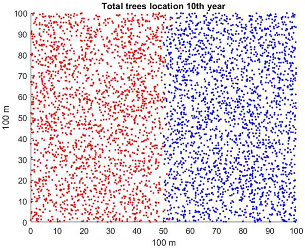
Figure 1. Typical starting conditions for invader (red) occupying the left-hand side of the plot and native (blue) occupying the right-hand side.
Two parameters are varied, the litter suppression parameter, slitter, and the mean dispersal distance parameter, c3. Increasing values of slitter are expected to favor the invader in competition. The values of c3 are varied, but are the same for the two species, so might intuitively be expected to have no net effect, but only speed up any process of spread, either by the invader or the native species population. The same sets of random number initiators were used for each value of c3, to eliminate random initial differences when comparing results for different values of c3, which means that for each simulation, the initial starting conditions were identical. Biocontrol is assumed to occur in this first of two applications. Without biocontrol, the growth and reproductive advantages of the invader result in it always dominating, even if slitter is set to zero (refer to Supplementary Figure A2.1 in Supplementary material for an example).
In contrast to the abovementioned scenarios that were initiated with similar age and size structures between the two species, each occupying half of the plot, the following scenarios, performed to study standing dead effects, assumed a random distribution of the native species. The initial total number of trees is distributed randomly in the 1-ha plot, with an initial total number of 2,000 trees randomly distributed, and is near to steady state. The invader starts from a small number of trees in the plot. The model plot was expanded to 120 × 120 m in the simulations to avoid possible numerical issues that could be caused by trees lying along one of the boundaries, e.g., part of the canopy lying outside the boundary. Only trees whose stems were within the 100 × 100 m region were included in the analysis.
We implement four scenarios where two species are randomly distributed in the 1-ha area. In the first scenario, we assume no biocontrol application. We set the initial invader population to 50. The native species population size is set to 2,000 and has age and dbh distributions indicative of a forest near steady state. We compare simulation outcomes without biocontrol but with and without standing dead. In the second scenario, standing dead trees are included in the simulations. In the third scenario, the initial population settings are equivalent to those of the first scenario, but biocontrol is introduced 80 years post-Melaleuca invasion. Finally, in the fourth scenario, we allow the native species to grow for a period of time without the invasive species to further guarantee a forest under a steady state. The native species undergoes succession, with an initial population size of 2,000 individuals, and in the absence of the invader for the first 100 years. The invader is introduced at a population size of 50 individuals, and biocontrol is commenced at year 180. Thus, biocontrol is applied 80 years post-invasion in scenarios 3 and 4. We try to keep the same sequence of the same initial setting for all four scenarios by using the same random number initiator. The model was implemented in MATLAB R2022a, and no specific toolbox was used.
The effects on competition of varying both the parameter slitter for the litter suppression of native seedlings and the parameter c3 for mean seedling dispersal distance can be summarized in a bifurcation diagram that shows a portion of the parameter space (Figure 2). As expected, for large values of slitter (>15), the invader is able to exclude the native for all values of c3. This occurs because high suppression allows the invading trees to substantially reduce the recruitment of native trees. Any sufficiently sizeable density of mature invader trees can suppress nearly all native seedlings. In contrast, for small values of slitter (< 11), the suppression of native seedlings cannot overcome the advantage of the native species in reproductive rate, so the native species tends to exclude the invader over the long run.
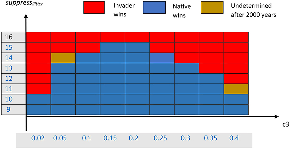
Figure 2. Bifurcation diagram for competition between the invading and native species. Red indicates that the invader appears to always exclude the native, blue indicates that the native appears to always exclude the invader, and brown indicates that it was not clear, after a long time period, which species would win.
However, the region of the parameter slitter from 11 to 15 is more interesting. In that region of parameter space, where the two species are more evenly matched in terms of their respective advantages, the winner is influenced by the mean dispersal distance, c3. This can be seen in the series of simulations in Supplementary Figures A2.2–A2.8 (Supplementary material) in which we look at a cross-section of values of c3 for the single value slitter = 14. For the cases shown, only three or four replicates with different random number initiators are shown, due to computational limitations. For very large mean seedling dispersal, c3 = 0.02, for which Supplementary Figure A2.2 is a typical example, the invader easily wins. It appears to be able to do that because it rapidly spreads seedlings to all the areas occupied by the native trees, and the litter suppression from the adult invasives is sufficient to reduce native seedling numbers to the extent that the invader can outcompete it so that it spreads into the native's original territory. The invader can build up litter densities up to 0.3 kg dry weight m−2 in some areas of the native's habitat, though most spatial cells have between 0.05 and 0.2 g m−2 (data not shown here).
At the opposite extreme, for small mean dispersal distances, c3 = 0.40 (Supplementary Figure A2.8), the invader is also on the way to winning. In this case, it appears that the invader wins by steadily advancing and spreading its seedlings only a slight distance ahead of the front, but in high enough density to preclude the native from the area around the front. This appears to be the case for c3 = 0.30 as well (Supplementary Figure A2.7), though it would require an impractically long simulation (+20 h) to confirm.
For the intermediate values of mean dispersal distance (roughly 0.05 ≤ c3 < 0.30), the situation is more complicated. The invader is not able to swamp the native with its own seedlings throughout the native's range. Some areas of the plot initially occupied by the native will receive only small input from invader seedlings. Because of biocontrol on the invader, the native has the advantage of a higher reproductive rate in those areas. That advantage will allow it to grow in those areas, even though the invader may be a superior competitor in other areas where its litter has reduced the native's recruitment. The invader also does not spread seedlings in sufficient density immediately ahead of the front to sufficiently suppress the native, so, for the same reason, the native is able to use its higher seedling production and growth rates to resist the invader. Although the native appears to be a clear winner for c3 = 0.10 (Supplementary Figure A2.4) and a likely winner for c3 = 0.15 and 0.20 (Supplementary Figures A2.5, A2.6), the competition is protracted, and only the directional tendency can be seen from these simulations. The results for c3 = 0.05 (Supplementary Figure A2.3) are the most interesting, as the outcome seems to be uncertain. Four different replicates produced different trajectories, only two of which were similar. In all these cases of intermediate values of c3, there are multiyear oscillations, suggesting that mechanisms other than simple demographic stochasticity are occurring. It is clear from Supplementary Figure A2.3 for c3 = 0.05 that, depending on the random number initiator, which sets the precise initial spatial location, age, and dbh of each of the 2,000 trees of each species, the trajectories differ to the extent that the winner can differ. This will be given more attention in the Section 4.
We found that sizedependence = 4 in Equation (3) yielded native species standing dead proportions like those observed in Florida hardwood and mixed hardwood forests. Our assumption means that, for example, a 100 cm dbh standing dead tree will occupy its location for 25 years; note, however, that its light interception will have been approximately zero after 4 years post-mortality (Supplementary Figure A1).
Four scenarios were used in the study of the effects of standing dead on the dynamics of the invader and native species. In scenario 1 without biocontrol, the invader excludes the native species in approximately 100 years if tree standing dead effects are not considered (Figures 3A, B). When standing dead trees are considered, the native species is still excluded but not completely until year 250 (Scenario 2, Figures 3C, D). The total living and standing dead tree abundance for both invading and native tree populations are shown in Figure 4A, and the ratios of standing dead to the total populations are shown in Figure 4B. As expected, the ratio of native standing dead rises to a high level as the population declines. The ratio of the invader standing dead rises and is steady at 0.15 as the population increases and dominates the vegetation. Equation (5) incorporates the assumption that smaller trees will remain standing for a shorter time after death. The maximum tree size in our model was 53 cm dbh. Therefore, from Equation (5) for residence time as a function of dbh, the longest mean time for removal of the standing dead agent would be 14 years. The minimum time predicted from Equation (5) was limited to 1 year, the time step of the model.
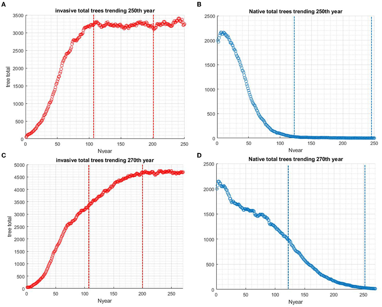
Figure 3. The presence of standing dead introduces a delay in the invasive species reaching carrying capacity. This also delays the native species from going to extinction. Scenario 1: (A) Without standing dead in the system, the population of invasive species takes approximately 100 years to reach carrying capacity. (B) Without standing dead in the system, the population decline of native species in 100 years. Scenario 2: (C) With standing dead in the system, the total population, including standing dead, of invasive species takes nearly 250 years to reach carrying capacity. (D) With standing dead in the system, the population decline of native species to extinction takes nearly 250 years.
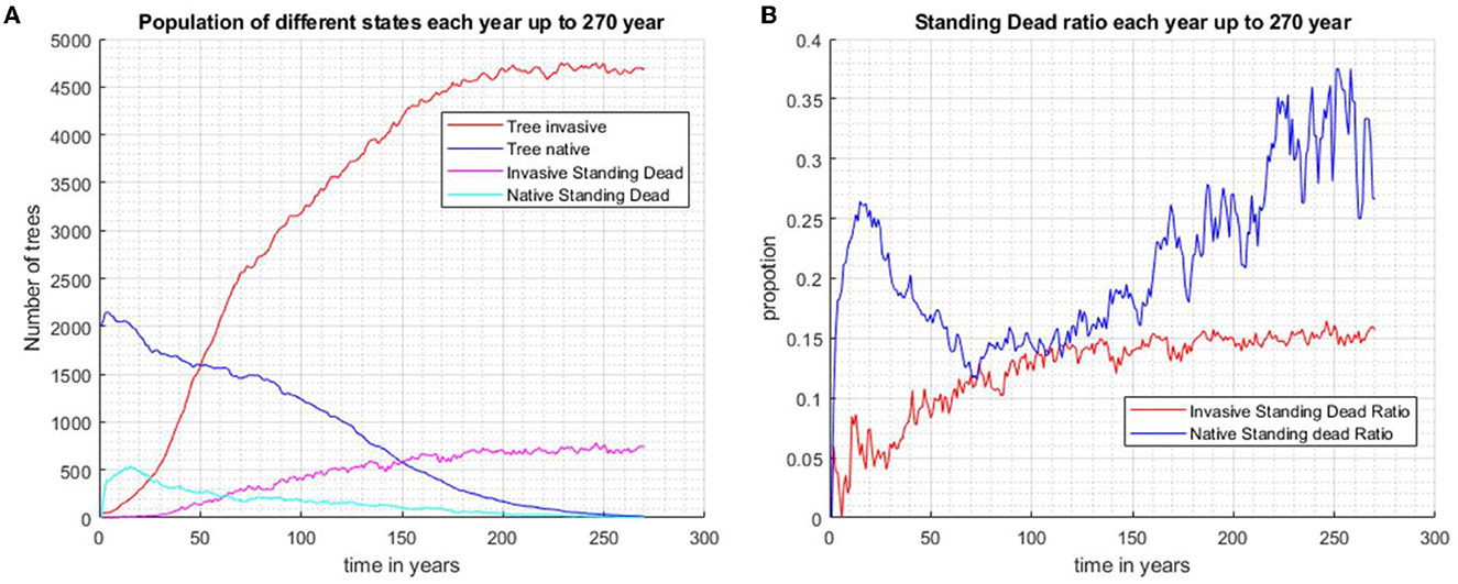
Figure 4. When the two species are randomly distributed across the same area initially and without biocontrol in the system, the invasive species outcompetes and occupies the entire plot after approximately 200 years (Scenario 2). (A) Population of invasive trees, native trees, invasive standing stand stems, and native standing dead stems. (B) The proportions of standing dead and the total population of each species.
This effect of tree size is reflected in the scenario where biocontrol is introduced at year 80. In scenario 3 (Figure 5B), the proportion of invader standing dead to total tree numbers peaks following biocontrol introduction, and the high proportion persists for only a few years. At 80 years (Supplementary Figure A2.4), the mean dbh of the invader is approximately 13 cm, and the median is approximately 5 cm, indicating that most invaders are small trees. The invader initially drives the native trees to low levels, but the imposition of biocontrol after 80 years leads to a gradual decline in the invader. After the commencement of biocontrol, the growth rate of the invader is suppressed by 80%, the reproduction rate declines by 90%, and young tree mortality increases; biocontrol leads to the eventual recovery of the native over 1,000 years (Figure 5A). The proportions of standing dead to the total population of both species fluctuate around similar values (Figure 5B).
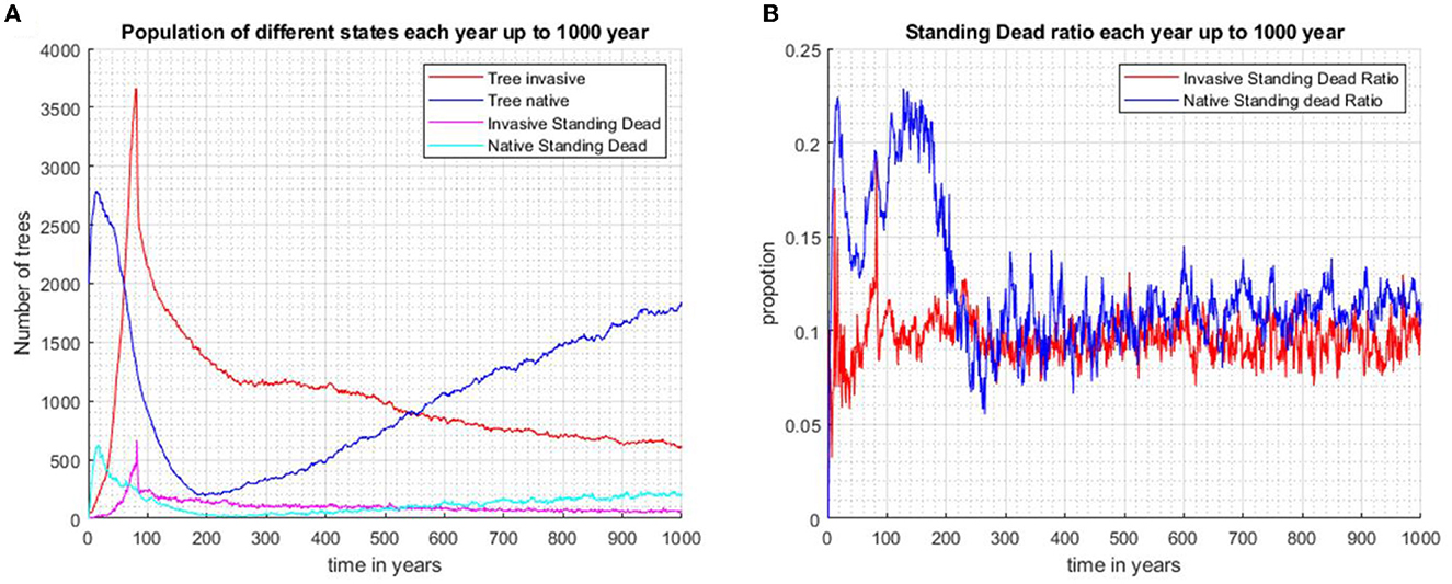
Figure 5. When the two species are initially randomly distributed across the same area and biocontrol is introduced after 80 years, the invasive species is seen to gradually decline and the community becomes mostly dominated by the increasing population of native species after 1,000 years (Scenario 3). (A) Population number of invasive trees, native trees, invasive standing stand stems, and native standing dead stems. (B) Proportions of standing dead and the total population of each species.
In scenario 3, there is a prolonged peak in the standing dead proportion for the native tree population after the introduction of the invaders and before biocontrol commenced (Figure 5B). The native trees are older and larger compared with invading trees. When outcompeted by the invaders, the natives' dead stems will, on average, persist on the landscape for a longer time. When the invader population starts to decline, the native trees recover and rebound to pre-invasion abundance. The standing-dead ratio remains steady at approximately 0.13.
In scenario 4 (Figures 6A, B), the native species is allowed to undergo natural succession in the absence of the invader for 100 years. This scenario differs from scenario 3 in that the native population is allowed time in the absence of the invader to build up to a population of close to 3,500 individuals and maintains a reasonable ratio of standing dead around 0.13 by the end of 100 years (Figure 6B). The invader, introduced at year 100, starts to suppress the native, but biocontrol, imposed at year 180, causes its decline. The native rebounds to close to 1,500 individuals after 1,200 years and continues a slow increase, while the invader continues a gradual decrease. The native species maintains a ratio of standing dead of close to 0.13, while the invader's standing dead ratio is only approximately 0.1 and tends to have more fluctuation while continuously decreasing. The results of the four scenarios are summarized in Table 1.
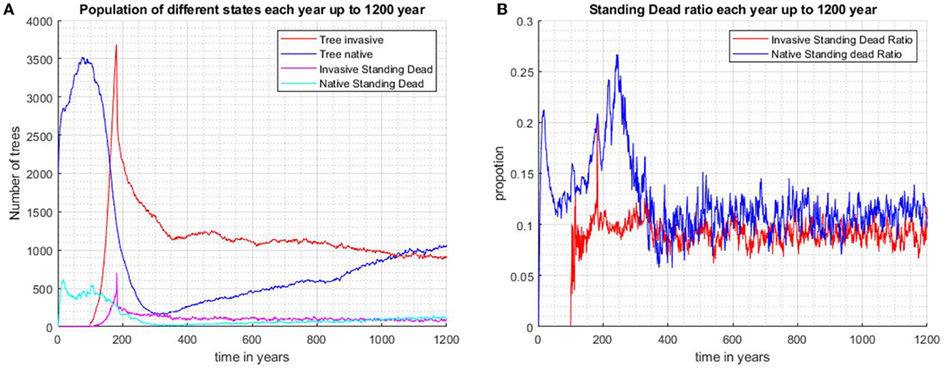
Figure 6. The native species is first allowed to run for 100 years before the invader is introduced as 100 randomly scattered individuals (Scenario 4). Biocontrol is introduced after 180 years. The invasive species is under control and the vegetation is mostly dominated by the increasing population of native species after 1,200 years. (A) Population number for invasive trees, native trees, invasive standing stand stems, and native standing dead stems. (B) Proportions of standing dead and the total population of each species.
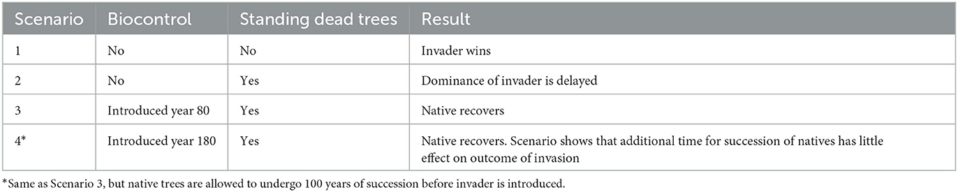
Table 1. Summary of four scenarios involving taking standing dead into account.
We used a spatially explicit agent-based model to explore questions concerning the effects of species properties on the competition between two species, one assumed to be an invader and the other a native species.
In our first application, we examined the combined effects of [1] biocontrol on the invader and [2] litter suppression of the native seedlings by invader litter, slitter, over a range of litter suppression coefficients and mean dispersal distances c3. We found that the results were complex for values of the litter suppression coefficient such that the advantages of the two species were relatively balanced. For such intermediate values of slitter (11 ≤ slitter ≤ 15), there seem to be three general regions along a mean dispersal distance axis, which have different qualitative population competition outcomes and different interpretations. We can interpret these different regions as follows.
• Very large mean dispersal distance (small c3). In this case, partly because the invader initially outnumbers the native in the number of trees, as it can tolerate greater stem density, it can spread many seedlings over the whole plot very quickly, such that, as adults, their litter suppresses the native seedlings and allows quick dominance of the invader. Refer to Supplementary Figure A2.2 for slitter = 14 with c3 = 0.02. It should be noted that the phenomenon was facilitated in our model by the limited size of the plot, which allowed invader seedling dispersal into all parts of the area occupied by the native. This could occur in small, relatively isolated stands of a native population. In larger plots, where seedlings cannot disperse to all areas of the plots, the dynamics might be as shown in step 3.
• At very low mean seedling dispersal distances (large c3), the invader spreads gradually, excluding the native along a slow-moving front. This mode of competition by a plant population has been likened to a phalanx attack, from the Greek “tactical formation consisting of a block of heavily armed infantry standing shoulder to shoulder in files several ranks deep” [refer to [30] for similar results in an analytic model of a clonal species]. For very short mean dispersal distances, the invader's seedlings fall close to its front line. This allows a very dense buildup of the invader at the front line. It does not advance very rapidly, but the native cannot stop the slow steady ‘grind it out' advance (refer to Supplementary Figures A2.7, A2.8 for slitter = 14 with c3 = 0.30 and 0.40). The case with c3 = 0.30 is especially interesting, as it is perhaps close to the borderline above which the phalanx effect succeeds. The native was far superior in numbers for approximately 1,000 years presumably because of its higher reproduction over the invader under biocontrol. However, eventually, the invader's short-range dispersal, combined with litter suppression by the invader, led to a phalanx effect, such that it slowly began to dominate (Supplementary Figure A2.7).
• At intermediate mean dispersal distances, the bio-controlled invader cannot rapidly saturate the whole plot with seedlings. The native will have spatial areas where it is relatively safe from invasion for long enough that it can use its higher reproductive rate to either gradually dominate or at least slow the invader's advance. Furthermore, the invader's seedlings are spread too thinly to constitute an effective phalanx. Supplementary Figures A2.4–A2.6, for slitter = 14 with c3 = 0.10, 0.15, and 0.20, show this over 2,000 years. The results appear to be relatively general, as they have three replications (a number limited by the long computer time for simulations). However, as Supplementary Figure A2.3 shows, stochasticity plays a major role in the outcome for the parameter c3 = 0.05. Replicate simulations for slitter = 14 with c3 = 0.05 showed that the winner varied, depending on the random number initiator. Clearly, stochasticity is playing a key role in the outcome of these simulations. However, the mechanism is not clear. In these cases, both populations remain large through the simulation, i.e., of the order of 2,000 individuals, so any effect of stochasticity in Supplementary Figure A2.3 does not resemble the usual small number effect of demographic stochasticity. There are coherent opposite-phase fluctuations of the two populations involving large numbers of individuals together over hundreds of years. This implies there is some sort of collective interactions affecting changes in population densities across spatial areas. It is possible that transient fluctuations in local population density can be self-amplifying for some period of time, but not always sustainable to the point of excluding one or the other species. A large number of individuals in the populations do not necessarily result in deterministic behavior.
As total population numbers of the invader and native are approximately the same over a long period of time in the figures with intermediate c3, before the populations start to diverge, one might ask if there are other signs, or early warning signals, in the data that could indicate which population would soon start to exclude the other. For the total populations shown in simulation in Supplementary Figure A2.3 for a random number initiator of 41, and for A2.9 for c3 = 0.05 and a random number initiator of Rand43, the spatial population distributions for years 600 and 1,200 years are shown in Figures 7A, B, respectively. Figure 7A shows the prelude to the takeover by the native, while Figure 7B shows the prelude to the takeover by the invader. The spatial distributions of the native and the invader at those times are complex. Both species are present in equal numbers in Figures 7A, B, but the winner is different in the two cases. Visually, there are certainly differences in spatial distributions that may anticipate the subsequent dynamics. It is possible that there are methods of analysis of the spatial patterns of the two species populations that may predict subsequent dynamics, as Eppinga et al. [31] suggested. The attempt to find quantitative measures of such difference that may be clues of the eventual winner will be the object of future study.
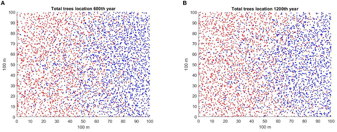
Figure 7. Spatial distributions of the native (blue) and invader (red) tree populations for the two simulations are shown in Figures A2.3, A2.9. In both cases, slitter = 14 and c3 = 0.05. (A) Spatial distribution for A2.3 at year 600, initial random number generator = 41, in which the native wins. (B) Spatial distribution for A2.9 at year 1,200, initial random number generator = 43, in which the invader appears to be winning.
The elucidation of the competition dynamics in the intermediate region in Figure 1 shows the power of ABM to reveal dynamics of a type not shown in traditional mathematical models of ecology. However, the simulations also show that there are regions where the dynamics are relatively deterministic; either the invader or the native rapidly excludes the other. That is true for both large (>15) and small (< 11) values of slitter. Within that region, the dynamics also seem relatively deterministic for cases of very large or very small c3 (small and large mean seedling dispersal). In all of these cases, it is likely that deterministic mathematical models can be constructed to describe the dynamics, as in Bolker and Pacala's [30] model of the phalanx effect in plant competition. However, as the simulations show, there are intermediate regions where such mathematical models, at least at their present state, are not sufficient to describe the dynamics. It might be argued that the intermediate parameter ranges, in which the two species are nearly evenly matched, are unlikely. However, there is modeling evidence that such species will converge to equal fitness [32], so there may be many cases for which mathematical models are sufficient. Kortessis et al. [18] studied the effects of litter suppression on competition, motivated by empirical data on the effect of invading grass species in the habitat of a native herbaceous species. Those authors found a range of trade-offs in competitive abilities for which stable coexistence could occur. We were unable to find any clear examples of stable coexistence in our model. Coexistence frequently lasted at least 2,000 years, but one or the other species was obviously increasing at the expense of the other in all such cases. It is possible that in the spatially explicit ABM, instabilities occur spatially that always prevent stable coexistence and lead to one or the other species driving the other toward extinction. However, we have not shown that conclusively.
As tree mortality increases across many forests globally, so should the frequency of standing dead trees [33]. Standing dead trees are integral components of forests, providing habitats for wildlife and housing a significant carbon pool [34, 35]. Forest models that incorporate standing dead trees focus on carbon retention and ecosystem processes [36, 37]. The role of standing dead in community-level dynamics, such as competition and invasion, has received much less attention. To the best of our knowledge, no mathematical model has incorporated standing dead trees to understand species interactions, and it would be difficult for them to do so in a realistic way. Competitive effects of dead trees are normally removed from ABMs under the assumption that dead trees no longer compete for limited resource [e.g., light [38, 39]]. We use a series of simplifying assumptions to include standing dead in a spatially explicit ABM.
Our findings show that standing dead trees can play a critical role in both invasion dynamics and the long-term trajectories of two competing species. The time it took the invading species to overtake the native species was delayed for 100 years in the model with standing dead trees (Figures 3A, C). In our model, standing dead has two functions: brief residual light interception and physical occupation of the forest floor that is proportional to the radius of the bole. As we parameterized rapid tree canopy decay post-mortality, i.e., light interception declined by > 90% after 1 year, standing dead effects are mostly driven by physical obstructions to seed rain and seedling establishment.
We sought to eliminate stochastic model effects during the first several decades since the individuals are assigned randomly in the plot and the density-dependent mortality function gives the forest a self-thinning effect [40]. The ratio of native standing dead increases at first for several years and stabilizes at 0.12 after 50 years. This ratio matches FIA data for the southern hardwood hammock forest. After the invaders and biocontrol are included, the invaders have a significant growth suppression of the native population at the invasion onset. To further investigate and validate, the pre-run model without commencement of biocontrol (Supplementary Figure A2.10) shows a similar result to scenario 1, after Melaleuca's invasion, the mixed forest has a higher standing dead ratio; it shows a proportion of 0.15 for native hardwood hammock. In general, the pre-run models yield similar forest dynamics and match well with the data from the southern hardwood hammock forest, which validate the standing dead effect free from the model instability.
High reproduction and growth rates of Melaleuca traits are characteristic of early successional stage species. These early successional communities tend to have higher invasive ability [41]. We simulated the age structure (Supplementary Figure A2.11) of the invasive forest when they first established, and it indicated that a large portion of this cohort consisted of smaller dbh (1.37–3 cm) stems. High invasion ability leads to competitive interaction when the invasive species establishes in a new habitat, resulting in disruptions in native species dynamics [42]. In our next application, we will further investigate the relationship between invasion ability and forest structure. Litter feedback on nutrient cycling (e.g., through differences in C:N ratios in invader's litter) can also facilitate invasion [43], which can be included in future modeling.
Our simplified approach to standing dead applies a novel, mechanistic component, i.e., dead trees have decaying light competition effects that persist a few years post-mortality. More recent agent-based forest simulator applications have applied behaviors to account for snag residences times, such as the “Snag Decay Class Dynamics” behavior in SORTIE-ND, which is based on Vanderwel et al. [44]. However, to the best of our knowledge, no applications have incorporated residual interactions that influence seedling establishment after canopy tree mortality.
The next step will be to investigate more complex scenarios of how vegetation responds to changes in tree canopy decay, light interception, and litter accumulation. Our simplifying standing dead assumption, residence time is proportional to dbh, does not fully capture complex snag dynamic processes. However, we believe it is reasonable because [1] most trees die standing in the absence of acute disturbances [i.e., not uprooted; [45–47]] and [2] many downed trees (at dbh) retain a root base that occludes future seedling establishment. Another addition will be competition reduction through branch mortality. Recent simulations have shown that branch mortality alters long-term forest stand structure and carbon cycling [48]. In addition, species traits affect snag decay times [49]. We assumed equal decay rates for each species. More complex modeling scenarios and future studies can include trait-dependent standing dead dynamics as well as residence times that depend on climate, soil substrate, and localized decomposition processes.
Broadly speaking, an objective of spatially explicit ABM is to model ecological systems more realistically by representing populations of discrete individuals, each of which can have its own properties and have local interactions with nearby individuals. However, we realize that ABMs are still idealizations of natural systems, and there are limitations on the degree to which they simulate real systems. Furthermore, mechanism-rich models such as what we have studied may require the estimation of numerous parameters. Paradoxically, the realism added by ABM also adds uncertainties in the estimation of additional parameters at the individual level, which is something for which mechanism-rich models are often criticized. However, the parameters of ABM are based on the solid foundation of physiology and traits of individual organisms, the likely ranges of which are generally known.
The modeling here suggests possible applications. Restoration efforts, in which native trees are replanted in areas in which invasives are being controlled, need guidance in maximizing the success of such efforts. ABM allows the simulation of different numbers and configurations of planting arrangements, which the modeling shows to be critical for success.
The original contributions presented in the study are included in the article/Supplementary material, further inquiries can be directed to the corresponding author.
DD developed the part of the model, performed the simulations, and wrote the parts of the manuscript. YL developed the parts of the model and performed the simulations. JX developed the parts of the model. LM performed the simulations and wrote the parts of the manuscript. All authors contributed to the article and approved the submitted version.
This work was funded by U. S. Geological Survey's Greater Everglades Priority Ecosystem Science Program.
We thank James Grace, Maarten Eppinga, and a reviewer for their very helpful comments. We are grateful to Daniel Johnson for helping with FIA data processing. Any use of trade, firm, or product names is for descriptive purposes only and does not imply endorsement by the U.S. Government.
The authors declare that the research was conducted in the absence of any commercial or financial relationships that could be construed as a potential conflict of interest.
All claims expressed in this article are solely those of the authors and do not necessarily represent those of their affiliated organizations, or those of the publisher, the editors and the reviewers. Any product that may be evaluated in this article, or claim that may be made by its manufacturer, is not guaranteed or endorsed by the publisher.
The Supplementary Material for this article can be found online at: https://www.frontiersin.org/articles/10.3389/fams.2023.1086781/full#supplementary-material
1. Skellam JG. Random dispersal in theoretical populations. Biometrika. (1951) 38:196–218. doi: 10.2307/2332328
3. DA A, Kareiva PM, Levin SA, Okubo A. Spread of invading organisms. Landscape Ecol. (1990) 4:177–88.
4. Hastings A, Cuddington K, Davies KF, Dugaw CJ, Elmendorf S, Freestone A, et al. The spatial spread of invasions: new developments in theory and evidence. Ecol Lett. (2005) 8:91–101. doi: 10.1111/j.1461-0248.2004.00687.x
5. Clark JS. Individuals and the variation needed for high species diversity in forest trees. Science. (2010) 327:1129–32. doi: 10.1126/science.1183506
6. Clark JS, Bell DM, Hersh MH, Kwit MC, Moran E, Salk C, et al. Individual-scale variation, species-scale differences: inference needed to understand diversity. Ecol Lett. (2011) 14:1273–87. doi: 10.1111/j.1461-0248.2011.01685.x
7. Hart SP, Schreiber SJ, Levine JM. How variation between individuals affects species coexistence. Ecol Lett. (2016) 19:825–38. doi: 10.1111/ele.12618
8. Marco DE, Páez SA, Cannas SA. Species invasiveness in biological invasions: a modelling approach. Biol Invas. (2002) 4:193–205. doi: 10.1023/A:1020518915320
9. Goslee SC, Peters DP, Beck KG. Spatial prediction of invasion success across heterogeneous landscapes using an individual-based model. Biol Invas. (2006) 8:193–200. doi: 10.1007/s10530-004-2954-y
10. Higgins SI, Richardson DM. A review of models of alien plant spread. Ecol Modell. (1996) 87:249–65.
11. Travis JM, Harris CM, Park KJ, Bullock JM. Improving prediction and management of range expansions by combining analytical and individualed modemodelling approaches. Methods Ecol Evol. (2011) 2:477–88. doi: 10.1111/j.2041-210X.2011.00104.x
12. Lu Y, DeAngelis DL, Xia J, Jiang J. Modeling the impact of invasive species litter on conditions affecting its spread and potential regime shift. Ecol Modell. (2022) 468:109962. doi: 10.1016/j.ecolmodel.2022.109962
13. Teh SY, DeAngelis DL, da Sternberg SL, Miralles-Wilhelm FR, Smith TJ, Koh H-L. A simulation model for projecting changes in salinity concentrations and species dominance in the coastal margin habitats of the Everglades. Ecol Modell. (2008) 213:245–56. doi: 10.1016/j.ecolmodel.2007.12.007
14. Kelleway JJ, Cavanaugh K, Rogers K, Feller IC, Ens E, Doughty C, Saintilan N. Review of the ecosystem service implications of mangrove encroachment into salt marshes. Glob Change Biol. (2017) 23:3967–83. doi: 10.1111/gcb.13727
15. Rayamajhi MB, Pratt PD, Tipping PW, Center TD. Litter cover of the invasive tree Melaleuca quinquenervia influences seedling emergence and survival. Open J Ecol. (2012) 2:131–40. doi: 10.4236/oje.2012.23016
16. Xiong S, Nilsson C. The effects of plant litter on vegetation: a meta-analysis. J Ecol. (1999) 87:984–94.
17. Facelli JM, Pickett ST. Plant litter: its dynamics and effects on plant community structure. Bot Rev. (1991) 57:1–32.
18. Kortessis N, Kendig AE, Barfield M, Flory SL, Simon MW, Holt RD. Litter, plant competition, and ecosystem dynamics: a theoretical perspective. Am Nat. (2022) 200:739–54. doi: 10.1086/721438
19. Holt RD, Barfield M, Gomulkiewicz R. Theories of niche conservatism and evolution: Could exotic species be potential tests. In:Sax D, Stachowitz J, Gaines SD, , editors. Species Invasions: Insights into Ecology, Evolution, and Biogeography. Sunderland, MA: Sinauer Associates (2005). p. 259–90.
20. O'Neal ES, Davis DD. Biocontrol of Ailanthus altissima: inoculation protocol and risk assessment for Verticillium nonalfalfae (Plectosphaerellaceae: Phyllachorales). Biocontrol Sci Technol. (2015) 25:950–69. doi: 10.1080/09583157.2015.1023258
21. Adler PB, D'Antonio CM, Tunison JT. Understory succession following a dieback of Myrica faya in Hawai'i Volcanoes National Park. Pac Sci. (1998) 52:69–78.
22. Esch CM, Kobe RK. Short-lived legacies of Prunus serotina plant–soil feedbacks. Oecologia. (2021) 196:529–38. doi: 10.1007/s00442-021-04948-1
23. Esch CM, Medina-Mora CM, Kobe RK, Sakalidis ML. Oomycetes associated with Prunus serotina persist in soil after tree harvest. Fungal Ecol. (2021) 53:101094. doi: 10.1016/j.funeco.2021.101094
24. Bennett JA, Franklin J, Karst J. Plant-soil feedbacks persist following tree death, reducing survival and growth of Populus tremuloides seedlings. Plant Soil. (2022)1–13. doi: 10.1007/s11104-022-05645-5
25. Talucci AC, Lertzman KP, Krawchuk MA. Drivers of lodgepole pine recruitment across a gradient of bark beetle outbreak and wildfire in British Columbia. Forest Ecol Manage. (2019) 451:117500. doi: 10.1016/j.foreco.2019.117500
26. Angers VA, Drapeau P, Bergeron Y. Snag degradation pathways of four North American boreal tree species. Forest Ecol Manage. (2010) 259:246–56. doi: 10.1016/j.foreco.2009.09.026
27. Oberle B, Ogle K, Zanne AE, Woodall CW. When a tree falls: controls on wood decay predict standing dead tree fall and new risks in changing forests. PLoS ONE. (2018) 13:e0196712. doi: 10.1371/journal.pone.0196712
28. Grimm V, Berger U, Bastiansen F, Eliassen S, Ginot V, Giske J, et al. A standard protocol for describing individual-based and agent-based models. Ecol Modell. (2006) 198:115–26. doi: 10.1016/j.ecolmodel.2006.04.023
29. Grimm V, Berger U, DeAngelis DL, Polhill JG, Giske J, Railsback SF. The ODD protocol: a review and first update. Ecol Modell. (2010) 221:2760–68. doi: 10.1016/j.ecolmodel.2010.08.019
30. Bolker BM, Pacala SW. Spatial moment equations for plant competition: understanding spatial strategies and the advantages of short dispersal. Am Nat. (1999) 153:575–602. doi: 10.1086/303199
31. Eppinga MB, Pucko CA, Baudena M, Beckage B, Molofsky J. A new method to infer vegetation boundary movement from ‘snapshot' data. Ecography. (2013) 36:622–635. doi: 10.1111/j.1600-0587.2012.07753.x
32. Scheffer M, Van Nes EH. Self-organized similarity, the evolutionary emergence of groups of similar species. Proc Natl Acad Sci USA. (2006) 103:6230–5. doi: 10.1073/pnas.0508024103
33. McDowell NG, Allen CD, Anderson-Teixeira K, Aukema BH, Bond-Lamberty B, Chini L, et al. Pervasive shifts in forest dynamics in a changing world. Science. (2020) 368:eaaz9463. doi: 10.1126/science.aaz9463
34. Franklin JF, Shugart HH, Harmon ME. Tree death as an ecological process. Bioscience. (1987) 37:550–6. doi: 10.2307/1310665
35. Woodall CW, Heath LS, Smith JE. National inventories of down and dead woody material forest carbon stocks in the United States: challenges and opportunities. Forest Ecol Manage. (2008) 256:221–8. doi: 10.1016/j.foreco.2008.04.003
36. Smith JE, Heath LS, Jenkins JC. Forest Volume-to-Biomass Models and Estimates of Mass for Live and Standing Dead Trees of US Forests. USDA Forest Service, Northeastern Research Station. NE-GTR-298, Newtown Square, PA (2003).
37. Woodall CW, Domke GM, Macfarlane DW, Oswalt CM. Comparing field-and model-based standing dead tree carbon stock estimates across forests of the US. Forestry. (2012) 85:125–33. doi: 10.1093/forestry/cpr065
38. Canham CD, Finzi AC, Pacala SW, Burbank DH. Causes and consequences of resource heterogeneity in forests: interspecific variation in light transmission by canopy trees. Can J Forest Res. (1994) 24:337–49.
39. Pacala SW, Canham CD, Saponara J, Silander JA Jr., Kobe RK, Ribbens E. Forest models defined by field measurements: estimation, error analysis and dynamics. Ecol Monogr. (1996) 66:1–43.
40. Berger U, Hildenbrandt H, Grimm V. Towards a standard for the individual-based modeling of plant populations: self-thinning and the field-of-neighborhood approach. Nat Resour Model. (2002) 15:39–54. doi: 10.1111/j.1939-7445.2002.tb00079.x
41. Rejmánek M. Invasibility of plant communities. In:Drake JA, Mooney HJ, Di Castri F, Groves RH, Kruger FJ, Rejmánek M and Williamson M, , editors. Biological Invasions: A Global Perspective. Chichester: John Wiley (1989) 369–388.
42. Dechoum MS, Castellani TT, Zalba SM, Rejmánek M, Peroni N, Tamashiro JY. Community structure, succession and invasibility in a seasonal deciduous forest in southern Brazil. Biol Invas. (2015) 17:1697–712. doi: 10.1007/s10530-014-0827-6
43. Eppinga MB, Molofsky J. Eco-evolutionary litter feedback as a driver of exotic plant invasion. Perspect Plant Ecol Evol Syst. (2013) 15:20–31. doi: 10.1016/j.ppees.2012.10.006
44. Vanderwel MC, Malcolm JR, Smith SM. An integrated model for snag and downed woody debris decay class transitions. Forest Ecol Manage. (2006) 234:48–59. doi: 10.1016/j.foreco.2006.06.020
45. Spies TA, Franklin JF. Gap characteristics and vegetation response in coniferous forests of the pacific northwest. Ecology. (1989) 70:543–5. doi: 10.2307/1940198
46. Aakala T, Kuuluvainen T, Grandpré LD, Gauthier S. Trees dying standing in the northeastern boreal old-growth forests of Quebec: spatial patterns, rates, and temporal variation. Can J Forest Res. (2006) 37:50–61. doi: 10.1139/x06-201
47. Esquivel-Muelbert A, Phillips OL, Brienen RJW, Fauset S, Sullivan MJP, Baker TR, et al. Tree mode of death and mortality risk factors across Amazon forests. Nat Commun. (2020) 11:5515. doi: 10.1038/s41467-020-18996-3
48. Needham JF, Arellano G, Davies SJ, Fisher RA, Hammer V, Knox RG, et al. Tree crown damage and its effects on forest carbon cycling in a tropical forest. Glob Change Biol. (2022) 28:5560–74. doi: 10.1111/gcb.16318
Keywords: biocontrol, standing dead trees, leaf litter, plant competition, spatially explicit, agent-based modeling
Citation: Lu Y, Xia J, Magee LJ and DeAngelis DL (2023) Seed dispersal and tree legacies influence spatial patterns of plant invasion dynamics. Front. Appl. Math. Stat. 9:1086781. doi: 10.3389/fams.2023.1086781
Received: 01 November 2022; Accepted: 13 February 2023;
Published: 23 March 2023.
Edited by:
Ivo Siekmann, Liverpool John Moores University, United KingdomReviewed by:
Sagar Adhurya, Kyung Hee University, Republic of KoreaCopyright © 2023 Lu, Xia, Magee and DeAngelis. This is an open-access article distributed under the terms of the Creative Commons Attribution License (CC BY). The use, distribution or reproduction in other forums is permitted, provided the original author(s) and the copyright owner(s) are credited and that the original publication in this journal is cited, in accordance with accepted academic practice. No use, distribution or reproduction is permitted which does not comply with these terms.
*Correspondence: Donald L. DeAngelis, ZGRlYW5nZWxpc0BtaWFtaS5lZHU=
Disclaimer: All claims expressed in this article are solely those of the authors and do not necessarily represent those of their affiliated organizations, or those of the publisher, the editors and the reviewers. Any product that may be evaluated in this article or claim that may be made by its manufacturer is not guaranteed or endorsed by the publisher.
Research integrity at Frontiers
Learn more about the work of our research integrity team to safeguard the quality of each article we publish.