What drives inflation and how? Evidence from additive mixed models selected by cAIC

We analyze the forces that explain inflation using a panel of 122 countries from 1997 to 2015 with 37 regressors. Ninety-eight models motivated by economic theory are compared to a boosting algorithm, non-linearities and structural breaks are considered. We show that the typical estimation methods are likely to lead to fallacious policy conclusions, which motivates the use of a new approach that we propose in this paper. The boosting algorithm outperforms theory-based models. Furthermore, we extend the current software implementation of conditional Akaike Information Criteria for additive mixed models with observation weights. We present a novel two-step selection process suitable for a wide range of applications that enables to empirically compare theory- and data-driven models with varying data availability.

1 Introduction

In the late 1970s and early 1980s, many countries experienced high inflation. A broad consensus emerged that this was unacceptable. Accordingly, policymakers worldwide adopted or were enabled to adopt policies designed to bring inflation down. As can be inferred from Figure 1, one of the most striking developments of the past two decades has been a steadily declining trend in inflation measured by consumer price index (CPI) and its volatility. In 1997, the average inflation was 21%. By 2015 it had dropped to 5%.

FIGURE 1

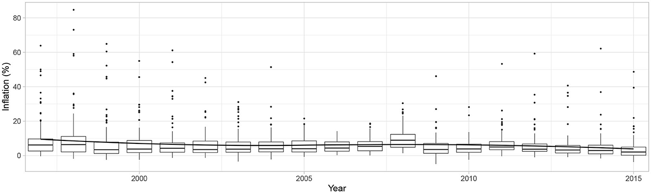
Figure 1. Truncated (99.5% percentile) distribution of inflation over time across 122 countries with a LOESS estimate.

Many factors are believed to have contributed to this development. They range from stronger commitments to price stability, improved monetary policy, the emergence of the New Economy and the attendant acceleration of productivity growth, forces of globalization that increased competition and enhanced the flexibility of labor and product markets, the weakening influence of trade unions, disciplined fiscal policy, favorable exogenous circumstances, and even luck. All these factors likely played a role, and disentangling the relative contribution of each remains an important challenge.

The general acceptance that the key objective of monetary policy should be price stability has aroused considerable interest in understanding the determinants of inflation. Empirical work in a cross-country setup is broad and diverse in its conclusions. Most of it addresses few potential sources for a limited number of countries or periods. Model comparisons are hardly made, and non-linearities have often not been analyzed. Robustness checks with alternative estimation techniques are rare. Moreover, commonly applied estimation methods are too restrictive and exhibit low explanatory power, which in the end may lead to fallacious policy conclusions. We corroborate this hypothesis in Appendix B.3, where we show that additive mixed models (AMMs) outperform common estimation techniques.

Empirical work that takes these shortcomings into account may help improve our understanding of what explains the inflation process over time and across countries. This offers the background to our paper, which identifies and quantifies various determinants of inflation, and motivates our extension of the empirical literature along several dimensions.

First, since the behavior of inflation has become increasingly difficult to understand,¹ we tested several models and variables based on abundant theoretical and empirical research. The explanatory variables were properly lagged to account for potential causal links.

Second, although the downward trend is a global phenomenon that had been noted years ago [3], research has typically focused on low-inflation (advanced) countries. For this reason, we base our analysis on not only as many theoretical explanations as possible but also the highest number of countries, including advanced countries, emerging market and developing economies (EMDEs), as well as low-income countries (LICs). To this end, we pre-processed and analyzed an exceptionally large and comprehensive data set, including annual observations of 37 explanatory variables for 122 countries during the period from 1997 to 2015.

Third, to properly consider the longitudinal structure of the data and the countries' heterogeneities, we recurred to mixed models whose variables were motivated by economic theory on the one hand and by a data-driven variable selection procedure on the other hand. Next, to allowing for a combination of countries with different characteristics, we extended the literature—which is focused on linear regressions, where inflation is regressed against a specific variable and control variables—by accounting for potential non-linear relationships between inflation and the regressors. For this purpose, we introduce additive mixed models to empirical research on inflation (which may find application in macroeconomic analyses in general) and provide the software implementation of conditional Akaike Information Criteria (cAIC) for additive mixed models with observation weights. The resulting assignment of cAIC to the models enabled us to compare several theories and the data-driven approach to one another.

The remainder of this paper is organized as follows. In Section 2 we review the literature and the ensuing explanatory variables underlying our empirical models. Section 3 presents the data. In Section 4 we lay out our estimation methods and the model selection procedure. The main findings are summarized in Section 5. Section 6 concludes the paper. Data and code for the reproduction of the analysis is available on a GitHub repository.

2 Literature

A number of empirical studies show that the sources of inflation are quite diverse and include excess demand or slack, a country's institutional set-up, the monetary policy strategy in place, fiscal imbalances, globalization and technology, demography, (shocks to) prices of natural resources, and past inflation. We discuss them in more detail, explain the choice of variables and their abbrevations for the empirical analysis in Appendix C. For an exhaustive survey of the literature we refer to Baumann et al. [4].

Based on this literature survey, we set up eight economic theories and various testable models, which capture a diversity of country characteristics. In the literature, money and output-related variables are often part of the explanatory variables. For this reason, they are also included in each of our models. Because it is not straightforward which variables best reflect the development of money stock and GDP, each model includes either M2 Gr. (%) or Credit (% GDP) Gr. (%) in combination with either GDP pc (USD) or GDP Gr. (%), extended by theory-specific explanatory variables. As a result, we obtained a range of four to 24 alternative specifications. This gave rise to an estimation of 98 model-specific variable combinations. The exact variable combinations of each economic model can be gleaned from the Appendix A. In addition to variable compositions suggested by economic theory, we also predefined interactions of variables for which we assumed the existence of a mutual impact on inflation. This applies to En. Prices (USD) and En. Rents (% GDP) as well as Trade Open. (% GDP) and Fin. Open.

3 Data

Our aim is to cover as many countries as possible. This entails a trade-off between the number of countries and the completeness of the data set. We were able to collect annual data running from 1995 to 2015 for 124 countries for 21 explanatory variables and for the dependent variable from publicly accessible sources, mainly the IMF and the World Bank. For inflation we finally relied on the IMF's change in the CPI due to data availability. Further, we derived growth rates from level variables, rolling averages from growth rate variables and further transformations from level variables. Thirty variables and the dependent variable resulted from this with missing information for some variables (2.8% of the observations). We imputed the missing observations by means of an EM-Algorithm on bootstrapped samples [5]. We limited the analysis to a single imputation instead of multiple imputed data sets due to the lack of theoretical background for averaging random effects. The contemporaneous measurements of the resulting variables were replaced by their 1- or 2-year lagged counterpart according to theory and empirical results.² We excluded two countries with outliers from our sample since these countries heavily impaired model selection. This led to 122 countries spanning from 1997 to 2015. We refer to these data as the full sample. In addition to the 30 variables, we also collected eight explanatory variables from various scientific publications and the World Bank that were not available across the whole time span from 1995 to 2015 or were only available for a subset of countries. Due to a non-compliance with the Missing At Random assumption these predictors were not imputed. These variables are associated with the economic theories Institutions, Monetary Policy Strategies, Public Finance, and Globalization and Technology. Their limited availability is one of the reasons for our two-stage selection procedure described in Section 4.5.

Finally, this gives rise to a classic longitudinal/panel data structure for a data set comprising 37 predictors and the World Bank's income classification. We provide summary statistics in the Appendix (cf. Figures A1, A2). According to the World Bank's income classification, ~21% of the countries are low-income countries, 35% belong to the lower-middle-income category, 19% to the upper-middle-income category, and 25% to the high-income category.

4 Methods

In this section we discuss the details of the statistical models and procedures underlying the analysis. First, we present the basic structure of AMMs on which we rely to model annual inflation rates. To capture the country-specific correlation and the heterogeneity of countries, we specify these AMMs with either subject-specific random or fixed effects and country-specific weights. All estimated AMMs are compared by their cAIC. We discuss the cAICs' central pillars in the context of AMMs and present our contribution to its software implementation in Section 4.2. We provide the details to model-based boosting for variable selection which we used as the starting point of our data-driven inflation modeling. We then present the two-stage model selection procedure that we developed. Finally, we add varying coefficients based on Hastie and Tibshirani [7] to the AMMs that exhibit the lowest cAIC to tackle the question of a structural break during the financial crisis 2007/2008.

4.1 Additive mixed models

Mixed models are a natural choice for modeling longitudinal data and have been frequently applied, for example, in epidemiology.³ However, to our knowledge, mixed models have not been applied to model inflation. In general, mixed models include (population) fixed and (subject-specific) random effects. When modeling macroeconomic data, a violation of the random effects assumption may arise, which eventually leads to inconsistent estimators For this reason, we apply a procedure proposed by Mundlak [10] to check if the random effects assumption holds or if random effects have to be replaced by country-specific fixed effects. In general, the country-specific effects should act as surrogates for effects that have not been measured and induce heterogeneity between countries. Further, since non-linear relationships between the many predictors used in this paper and inflation cannot be excluded, we extend the mixed models in an additive manner by model terms which are functional forms of the predictors. This leads to the class of AMMs on which our main analysis is based.

The formal structure of the AMMs is as follows: 37 (metric and categorical) predictors and the dependent variable inflation (in percent), denoted by ỹ_{i, t}, are given for i = 1, …, n = 122 countries and for t = 0, …, T = 18 consecutive years from 1997 to 2015 such that ${ỹ}_i={({ỹ}_{i,0},\dots ,{ỹ}_{i,\mathcal{T}})}^{\top }$. The vector $\tilde{y}={\left({\tilde{y}}_1{}^{\top },\dots ,{\tilde{y}}_n^{\top }\right)}^{\top }$ has been transformed by the natural logarithm y: = ln(ỹ+10.86) after shifting the support to values ≥1 to avoid numerical instabilities. We chose the natural logarithm transformation to meet the distributional assumptions specified for ϵ_i in (1). The generic AMM used to explain y_{i, t} by a set of predictors A_{j, l} is given in Equation (1). Each of the eight economic theories is represented by a set G_l: = {{A_{1, l}}, {A_{2, l}}, …, {A_{ml, l}}}, l = 1, …, 8, containing m_l: = ∣G_l∣ sets of predictors A_{j, l}. Each A_{j, l} is composed of disjunct subsets B_{j, l} and C_{j, l} of predictors with linear and non-linear effects, respectively, as well as pairs D_{j, l} of variables in B_{j, l} and pairs E_{j, l} of variables in C_{j, l} with linear and non-linear interaction effects, respectively. Non-linear effects h of predictors x∈C_{j, l} are estimated by univariate cubic P-splines [11] with second-order difference penalties. Interaction effects f(·, ·) of pairs (x, x^*) of variables in E_{j, l} are modeled using penalized bivariate tensor-product splines. The assignment to B_{j, l}, C_{j, l}, D_{j, l} and E_{j, l} can be found in Tables A1, A2. Each model M_{j, l} corresponding to one A_{j, l}∈G_l is of the following form:

$\begin{array}{ll}{y}_{i,t}={\beta }_0+{\eta }_{i,t}+Z_{i,t}{b}_i+{ϵ}_{i,t},& (1)\end{array}$

$\begin{array}{l}{\eta }_{i,t}={\displaystyle \sum _{x\in B_{j,l}}{x}_{i,t}}{\beta }_x+{\displaystyle \sum _{(x,x^{*})\in D_{j,l}}(x_{i,t}{x}_{i,t}^{*})}{\beta }_{(x,x^{*})}+{\displaystyle \sum _{x\in C_{j,l}}{h}_x}(x_{i,t})\\ +{\displaystyle \sum _{(x,x^{*})\in E_{j,l}}{f}_{(x,x^{*})}}(x_{i,t},x_{i,t}^{*})& (2)\end{array}$

with $b_i={(b_{i,0},b_{i,1})}^{\top }\stackrel{iid}{~}\mathcal{N}(0,G)$, where a random intercept b_{i, 0} and a random slope b_{i, 1} with design vector Z_{i, t}≡Z_t = (1, t) and non-diagonal covariance G are (always) included to capture the serial within-country correlation. Further, ϵ_i~N(0, R_i) is assumed with ϵ_i⊥⊥b_i, where R_i is a diagonal matrix with potentially heterogeneous country-specific variances ${\sigma }_i^2$ on its diagonal. The observation weights $w_i={\sigma }^2/{\sigma }_i^2$ emerge implicitly and are contained on the diagonal of the matrix ${\tilde{W}}_i$ such that $R_i={\sigma }^2{\tilde{W}}_i^{-1}$. On a sample level, the error covariance structure is a block-diagonal matrix R with R_i on its diagonal.

Assuming ϵ_i⊥⊥b_i further implies that the b_i have to be uncorrelated with all x_{i, t} and $x_{i,t}^{*}$ included in the subsets of A_{j, l} for all t. This assumption may seem unreasonable given the data and question under investigation. For this reason, we question the random effects assumption (i.e., $E\left[b_i|x_{i,t},x_{i,t}^{*}\right]=E\left[b_i\right]$ for all t) and alternatively specified country-specific fixed effects to take the country-specific correlations into account. Specifically, we alternatively specified each M_{j, l} as in (1) but without any distributional assumption for the country-specific parameters:

$\begin{array}{ll}\begin{array}{l}{y}_{i,t}={\eta }_{i,t}+Z_{i,t}{\gamma }_i+{ϵ}_{i,t},\hfill \end{array}& (3)\end{array}$

where ${\gamma }_i={({\gamma }_{i,0},{\gamma }_{i,1})}^{\top }$. To decide if the random effects assumption under (1) or the country-specific fixed effects under (3) are more reasonable for each M_{j, l}, we follow Mundlak [10], whose procedure enables us to derive a statistical test which examines if the time-invariant error components of the error in (1) might not be correlated with the time-varying regressors specified in (2). We test this hypothesis by specifying a further model ${\bar{\mathcal{M}}}_{j,l}$ for each M_{j, l} which is specified as the corresponding M_{j, l} but with a linear predictor ${\bar{\eta }}_{i,t}$ that additionally encloses the time-averaged transformations of the regressors (i.e., ${\bar{x}}_i=\frac{1}{\mathcal{T}+1}\sum _{t=0}^{\mathcal{T}}{x}_{it}$) specified in (2). As a result, each ${\bar{\mathcal{M}}}_{j,l}$ is of the form

$\begin{array}{ll}\begin{array}{l}{y}_{i,t}={\beta }_0+{\overline{\eta }}_{i,t}+Z_{i,t}{b}_i+{ϵ}_{i,t},\hfill \end{array}& (4)\end{array}$

$\begin{array}{l}{\overline{\eta }}_{i,t}={\eta }_{i,t}+{\displaystyle \sum _{x\in B_{j,l}}{\overline{x}}_i{\overline{\beta }}_{x_B}}+{\displaystyle \sum _{(x,x^{*})\in D_{j,l}}{\overline{x}}_i{\overline{\beta }}_{x_D}}+{\overline{x}}_i^{*}{\overline{\beta }}_{x_D^{*}}+{\displaystyle \sum _{x\in C_{j,l}}{\overline{x}}_i{\overline{\beta }}_{x_C}}\\ +{\displaystyle \sum _{(x,x^{*})\in E_{j,l}}{\overline{x}}_i{\overline{\beta }}_{x_E}}+{\overline{x}}_i^{*}{\overline{\beta }}_{x_E^{*}}& (5)\end{array}$

We test if all the parameters of the time-averaged transformations of the regressors are jointly zero, i.e., ${\mathcal{H}}_0:{\bar{\beta }}_{x_{\mathcal{B}}}={\bar{\beta }}_{x_{\mathcal{D}}}={\bar{\beta }}_{x_{\mathcal{D}}^{*}}={\bar{\beta }}_{x_{\mathcal{C}}}={\bar{\beta }}_{x_{\mathcal{E}}}={\bar{\beta }}_{x_{\mathcal{E}}^{*}}=0$ against the alternative H_A, that at least one of these parameters differs from zero based on a likelihood-ratio test (cf. Appendix B.1). When we could not reject H₀ at the 5%-significance level, we favored the specification under (1) over (3) for the corresponding M_{j, l}. We interpret the test result as an indication rather than a statement that provides definitive certainty for the choice between fixed and random effects.

In total, there are 98 (= $\sum _{l=1}^8{m}_l$) such AMMs for all predictor sets A_{j, l} associated with each economic theory G_l. For each G_l there is one set of models ${\mathcal{M}}_l$ which includes all corresponding M_{j, l}. We estimated these AMMs by (penalized) maximum likelihood with the mgcv package [12] and the gamm4 package [13] as extensions to the statistical software R [14].

The typical working horse model for studying inflation is the vector autoregressive (VAR) model as used, for example, by Karlsson et al. [15]. However, we prefer AMMs over VAR models for two reasons. The first is that AMMs can be parameterized more parsimoniously, given the large number of predictors (37) and countries (122) underlying our analysis. The second reason is that AMMs do not require any specification of the time lag order of the variables, contrary to VAR models.

4.2 cAIC

Model selection based on the Akaike information criterion (AIC) is a common approach in econometrics. The criterion was initially introduced by Akaike [16] and is composed of twice the maximized log-likelihood and a bias correction term, which, under certain regularity conditions, can be estimated asymptotically by two times the dimension of the unknown parameter vector specifying this log-likelihood [17]. To apply this criterion to mixed models, two considerations were taken into account in our case.

First, a joint Gaussian distribution of the random vectors y and b is assumed. This allows us to decide between two common views regarding the inference and predictions in mixed models. The distribution of y cond. on b leads to the cond. likelihood of y given b, which then forms one component of our utilized cAIC. In contrast, when the random effects are integrated out, the marginal distribution of y emerges and thus provides the marginal likelihood. We demonstrate our reasoning for the conditional over the marginal view on the AIC in Section 4.3.

Second, the bias correction term needs to be adjusted owing to the alternated number of parameters estimated in mixed models. A body of literature [18–20] provides the theoretical underlying for the derivation of the bias correction. We give a brief overview in Section B.2 in the Appendix. We base our analysis on the term introduced by Greven and Kneib [20] [cf. (3) in the Appendix], which assumes independent and identically distributed errors across the subjects (countries in our case). As a result, its current software implementation in the cAIC4 package [21] originally provided for mixed models emerging from the lme4 package [22] and the gamm4 package [13] incorporates this assumption as well. However, in our case subject-specific error variances need to be modeled to capture the heterogeneity across countries, making the assumption of identically distributed errors inappropriate. The derived bias correction is thus no longer applicable since it disregards the additional parameters used for the estimation of R as defined in Section 4.1. In order to account for the estimation of a more complex error covariance structure in the bias correction, we incorporate the proposed extension of Overholser and Xu [23]. Since Overholser and Xu do not take into account the estimation uncertainty of G, we implemented a working version that adds the number of unknown parameters r, which we used for the estimation of the error covariance matrix R, to the bias correction term of (3) in the Appendix and obtained

$\begin{array}{ll}\text{cAIC}=-2\text{log}f(y|\theta ,b)+2\left(\text{tr}\left(\frac{\partial ŷ}{\partial y}\right)+r\right).& (6)\end{array}$

We implemented Overholser and Xu's proposal for diagonal error covariance matrices into the cAIC4 package and further extended the package for mixed and additive models estimated with the mgcv package [12]. As a result, we provide, to our knowledge, the first software implementation for the estimation of the cAIC for mixed and additive models with non identically distributed errors. This novel extension of cAIC4 is made available to the CRAN repository for further applications. The proof of the asymptotic result of Overholser and Xu [23] gives an upper bound for the bias correction term that can also be provided through derivations based on the partial derivative of the prediction vector ŷ for y with the random effects set to their predicted values.

4.3 Conditional over the marginal view on the AIC

We prefer the conditional over the marginal perspective on the AIC due to the mixed model representation of P-splines. To see the link in general, following Saefken et al. [17], we consider an additive model of the following form

$\begin{array}{ll}\begin{array}{l}y=Ba+\epsilon ,\epsilon ~N(0,{\sigma }^{2}I)\hfill \end{array}& (7)\end{array}$

where B is the design matrix containing the evaluations of predictors based on B-spline basis functions constructed from piece-wise polynomials and a is the corresponding vector containing the basis coefficients. We can apply an eigenvalue decomposition to the quadratic penalty matrix P = D^⊤D with column rank k, where D is the differences matrix such that $P=V\tilde{\Sigma }{V}^{\top }$. The k eigenvectors in V, which correspond to the k positive eigenvalues, can be assigned to V₁ while the remaining d column vectors can be assigned to V₀. We are then able to non-uniquely decompose the functional estimate Ba into two bases

$\begin{array}{ll}\begin{array}{l}Ba=B{V}_0{V}_0^{\top }a+B{V}_1{V}_1^{\top }a=X\beta +Zb\hfill \end{array}& (8)\end{array}$

yielding the common mixed model representation [24], where β specifies d unpenalized parameters with the corresponding fixed effects design matrix X spanning the polynomial null space of P, while b specifies k penalized parameters corresponding to the random effects design matrix Z which spans its complement [25], respectively. Currie et al. [26] extend this representation for penalized functionals in higher dimensions. The specification under (8) differs from our generic mixed model (1) by different column ranks of the fixed and random design matrices and different dimensions of the corresponding parameter vectors, depending on the employed predictor sets A_{j, l} as defined in Section 4.1. As a result, with d = 2 in our case, the marginal AIC would only take the fixed polynomial trend of degree one into account while the smooth deviation from this polynomial can now be taken into account in (6) as well. Thus, the cAIC, considered as a predictive measure in this context, accounts for the plausible assumption that the non-linear functional relation between the predictors and y estimated in our data set represents a more general relationship which is expected to hold also for new country observations.⁴

4.4 Model-based boosting

In order to maximize predictive performance on out-of-sample data, we in addition relied on a machine learning approach which could also be used for forecasting purposes. Specifically, we apply a model-based boosting algorithm [27–29]. It disregards the block by block segmentation of the predictors presented in Section 2, which was based upon the associated economic theories. For this reason, we next want to find an optimal prediction function f^* for y through some prediction function f which is found by minimizing the expected loss ᵔ_{Y, X}[𝒧(y, f(x))] (i.e., risk) through a gradient descent algorithm in function space [28]. We assume that f is composed of a sum of functions of predictors and country-specific random effects which are all parameterized through different base learners. We specified 34 base learners. We now discuss the employed loss function, the choice of base learners, the gradient descent algorithm and the base learner selection procedure.

4.4.1 Loss function

The boosting algorithm minimizes the empirical risk which is given by

$\begin{array}{ll}ℛ=\frac{1}{n}{\displaystyle \sum _{i=1}^n\mathcal{L}}(y_i,f(x_i))& (9)\end{array}$

where (y_i,x_i) is one out of i = 1, …, n realizations of (y,x). The Huber-Loss, 𝒧, was chosen because of its advantages in handling outliers compared with other approaches. The Huber-Loss is defined as

$\begin{array}{ll}\mathcal{L}(y,f;\delta )=\{\begin{array}{l}\frac{1}{2}(y-f)2\text{ for }|y-f|\le \delta ,\\ \delta (|y-f|-\frac{\delta }{2})\text{ for }|y-f|>\delta \end{array}& (10)\end{array}$

and δ was chosen in each boosting iteration m by

$\begin{array}{l}{\delta }_m=\text{median}(|y_i-{\widehat{f}}_{m-1}|,i=1,...,n).\end{array}$

4.4.2 Base learners

All predictors specified in Section 2 which are available in the full sample were collected in x: = (x₁, …, x_p). For the case of inflation, four kinds of base learners are specified. The first type are penalized least squares base learners which model all categorical predictors in x. The second type are P-spline base learners which model all continuous predictors in x. The third type are bivariate P-splines base learners allowing for the estimation of smooth interaction surfaces. We allow for the same bivariate interactions of predictors as we have done for the models specified by economic theory—En. Prices (USD) and En. Rents (% GDP) denoted by f_{1, 2} and Trade Open. (% GDP) and Fin. Open. denoted by f_{3, 4}. The last type are random effect base learners for country-specific random intercepts, f_intercept, and country-specific random slopes, f_slope, with Ridge-penalized effects. We finally add a global intercept such that the following additive model results

$\begin{array}{ll}𝔼\left[y|x\right]={\beta }_0+f_1+\dots +f_p+f_{1,2}+f_{3,4}+f_{intercept}+f_{slope}.& (11)\end{array}$

4.4.3 Gradient descent algorithm

The utilized gradient boosting algorithm starts with an initial function estimate ${\widehat{f}}_{\left[0\right]}$ and proceeds in a stagewise manner. At each iteration m it computes the negative gradient of the loss function and updates the current function estimate ${\widehat{f}}_{\left[m\right]}^{*}$. Simultaneously, the algorithm descends along the gradient of the empirical risk ℛ whereby only one base learner is selected at each iteration for updating the current function estimate. The decision when to stop the algorithm, m_stop, is crucial. However, it has been commonly suggested to enforce a stop of the algorithm before it converges to avoid overfitting and thus a suboptimal prediction [27].

4.4.4 Base learner selection

We employ a 10-fold bootstrap to find m_stop by choosing the minimum out-of-sample risks averaged over all folds [29]. To take the longitudinal structure of our data into account this procedure was stratified by countries. To enforce variable selection, we decided to include only the base learners that were selected at least 1% of all m_stop iterations. Finally, 14 out of the 34 base learners were selected. By stopping the algorithm before it converges, a shrinkage effect is imposed onto the effect estimates of the model. Therefore, we refitted the predictors associated with the 14 base learners collected in the predictor set A_B as an AMM as specified in (3) and dubbed it M_B. We favored (3) over (1) due to the result of the testing procedure proposed by Mundlak [10].

4.5 Selection procedure

The model selection procedure is as follows: At a first stage ${\mathcal{S}}_{fir}$, a winner model ${\mathcal{M}}_l^{*}$ with the lowest cAIC (6) among models M_{j, l} in the set ${\mathcal{M}}_l$ is selected for each economic theory. At a second-stage, ${\mathcal{M}}_l^{*}$, l = 1, …, 8 and M_B are collected in the set ${\mathcal{M}}_{\mathcal{P}}$. Some predictors associated with ${\mathcal{M}}_2$, ${\mathcal{M}}_3$, ${\mathcal{M}}_4$ and ${\mathcal{M}}_5$ are not imputed as these predictors are not available either across time and/or countries which makes a direct model comparison by means of the Likelihood and thus the cAIC invalid. As a result, if the predictor sets included in ${\mathcal{M}}_2^{*}$, ${\mathcal{M}}_3^{*}$, ${\mathcal{M}}_4^{*}$ and ${\mathcal{M}}_5^{*}$ are only available for a subsample of data, they are instead added to ${\mathcal{M}}^{{}^{″}}$ to be compared to the AMM with the lowest cAIC in ${\mathcal{M}}_{\mathcal{P}}$ later. The winner M_P has the lowest cAIC in the set of models ${\mathcal{M}}_{\mathcal{P}}$ and its cAIC is finally compared to each ${\mathcal{M}}^{{}^{″}}\in {\mathcal{M}}^{{}^{″}}$ on the corresponding different data subsets to yield the overall winner M^**. If the computation of any AMM on any subset of the data fails, this AMM is assigned the highest cAIC in the given comparison. This can happen in particular for complex models on smaller subsets of the data. First- and second-stage selection are together labeled ${\mathcal{S}}_{sec}$. M^** represents the model with the highest empirical relevance and provides the most reasonable set of inflation drivers.

The reasoning behind this two-stage approach is twofold. First, from a monetary economics perspective it is not known a priori which set of predictors has the most explanatory power for each economic theory (G_l). Second, the availability of certain predictor sets A_{j, l} across time and countries enforces this procedure to ensure an admissible model comparison by means of the Likelihood and thus cAIC.

4.6 Varying coefficient models

After the model selection procedure, we additionally answered the important question of a structural break for the parameters comprised by ${\mathcal{M}}_l^{*}$, l = 1, …, 8 and M_B through varying coefficient models. That is, we let each parameter interact with a two-level categorical variable e_{i, t, k} which is coded with e_{i, t, 1} = 1_{t ≤ 2007} and e_{i, t, 2} = 1_t>2007 such that (2) was replaced by

$\begin{array}{l}{\overline{\eta }}_{i,t}=-{\beta }_0+{\displaystyle \sum _{k\in \{1,2\}}({\beta }_{0,k}{e}_{i,t,k}+{\displaystyle \sum _{x\in B_{j,l}}{x}_{i,t}}{\beta }_{x,k}{e}_{i,t,k}+{\displaystyle \sum _{(x,x^{*})\in D_{j,l}}(x_{i,t}{x}_{i,t}^{*})}{\beta }_{(x,x^{*};k)}{e}_{i,t,k}}\\ +{\displaystyle \sum _{x\in C_{j,l}}{h}_{x,k}}(x_{i,t})e_{i,t,k}+{\displaystyle \sum _{(x,x^{*})\in E_{j,l}}{f}_{(x,x^{*};k)}}(x_{i,t},x_{i,t}^{*})e_{i,t,k})& (12)\end{array}$

for each ${\mathcal{M}}_l^{*}$, l = 1, …, 8 and M_B. The first level of e_{i, t} is considered when t ≤ 2007 and the second level when t>2007. Consequently, we obtain two simultaneous estimations of the same effect—one for each of the two levels. However, apart from the specification of (12), every model specification was identical to the model specification of the original ${\mathcal{M}}_l^{*}$, l = 1, …, 8 or M_B, respectively.

5 Results

The results of the AMMs presented in Section 4 are discussed in this section which is organized in two subsections. In the first, we present the results of ${\mathcal{S}}_{fir}$ as described in Section 4.5. Ordered by theory, we present the winning models, ${\mathcal{M}}_l^{*}$, assessed by their cAIC and the resulting variables, discuss the linear links and plot the pattern of the variables that were estimated as P-splines together with their pointwise 95% confidence intervals [30]. The empirical degree of non-linearity is assessed based on the effective degrees of freedom [EDFs; [31]] associated with each penalty specified in (2). The EDFs are reported along the y-axis. For example, an EDF equal to 1 indicates that the estimated M_{j, l} penalized the corresponding smooth term to a linear relationship. To solve the identifiability issue of the AMMs specified in Section 4.1, all splines estimated incorporate a sum-to-zero constraint [e.g., $\sum _{i,t}{ĥ}_{\mathcal{G}\mathcal{D}\mathcal{P}pc(\mathcal{U}\mathcal{S}\mathcal{D})}(\mathcal{G}\mathcal{D}\mathcal{P}pc{(\mathcal{U}\mathcal{S}\mathcal{D})}_{i,t})=0$ for M_{6, 1}]. As a result, the corresponding effects can only be interpreted on a relative scale. In addition, for each model term enclosed by either (2) or (12) we performed a statistical test [30], where under the null the parameters associated with this model term are equal to zero. The order of magnitude of the p-value associated with this test is reported by means of asterisks.⁵ Simultaneously, we evaluate the existence of structural breaks in the wake of the financial crisis and juxtapose the evidence of the pre-crisis period with that after the crisis. To this end we applied the varying coefficient approach as defined in Section 4.6. As discussed in Sections 3 and 4.5, not all models could be estimated and compared on the full sample. The models included in ${\mathcal{M}}_1$, ${\mathcal{M}}_2$, ${\mathcal{M}}_6$, ${\mathcal{M}}_7$ and ${\mathcal{M}}_8$ were fitted on the maximum of observations possible.

For the estimates of the institutional characteristic ${\mathcal{M}}_2$, we fitted the model on 26 countries and for a time span from 2000 to 2012 at the first stage due to the missing structure of the predictors as described in Section 3. However, we refitted ${\mathcal{M}}_2^{*}$ on the full sample at the second stage since the predictors attached to its predictor set, A_{16, 2}, are available for all 122 countries and all 19 points in time. The models examining monetary policy strategy variables, ${\mathcal{M}}_3$, were fitted on 30 countries and a time interval from 1997 to 2012. The models examining effects from public finance, ${\mathcal{M}}_4$, were fitted on 79 countries from 1997 to 2015. The AMMs enclosed by ${\mathcal{M}}_5$, that is globalization and technology, were fitted on 93 countries and from 1997 to 2012. Since the predictors, A_{3, 3}, A_{14, 4} and A_{20, 5}, are not available in the full sample, ${\mathcal{M}}_3^{*},{\mathcal{M}}_4^{*}$ and ${\mathcal{M}}_5^{*}$ were excluded from ${\mathcal{S}}_{sec}$.

In the second subsection, we describe the results of ${\mathcal{S}}_{sec}$ which were characterized by the addition of M_B to the winners of ${\mathcal{S}}_{fir}$. Here, we identify the overall winning model, M^**, and describe its links to log inflation.

5.1 First stage selection

This subsection describes the results organized by economic theory. It first presents the winning model within the estimated model combinations and compares the empirical relevance of the variables involved. The winning model is characterized by the lowest cAIC value. Tables A1, A2 display the results divided by theory. The first section lists the results for money, credit and slack, ${\mathcal{M}}_1$, the second section those for institutions ${\mathcal{M}}_2$, the third for monetary policy strategies, ${\mathcal{M}}_3$, the fourth for public finance ${\mathcal{M}}_4$, the fifth for globalization and technology, ${\mathcal{M}}_5$, the sixth for demography, ${\mathcal{M}}_6$, the seventh for natural resources, ${\mathcal{M}}_7$, and the eighth for past inflation, ${\mathcal{M}}_8$. As can be gleaned from the p-values reported in Tables A1, A2, we specified country-specific fixed effects rather than random effects if the tested hypothesis specified based on the proposal of Mundlak [10] in Section 4.1 was significant at the 5% level. The results were rounded to the second digit. In case of a value below 0.01, the results were rounded to 0.01. Similarly, in case of a value >0.99, the results were rounded to 0.99.

The subsequent discussion focuses on whether the effects are linear or not, based on the EDF values. Three figures plot the results for three different periods of observations. A left-hand panel plots the results for the whole sample, a middle panel those relating to the pre-crisis and a right-hand panel those for the post-crisis period.

5.1.1 Money, credit, and slack

AMMs that include M2 growth exhibit higher empirical relevance than those that include credit growth, while the models that include output gap are more relevant than those that account for GDP growth. However, the output gap is less relevant than GDP pc. M_{6, 1} is the winning model. It exhibits GDP pc and credit growth. There is evidence of a linear and positive association between credit growth and log inflation. A one percentage point increase leads to a rise in log inflation of 0.022^* (~2.2% increase in inflation). The estimated effect after the global financial crisis (GFC) (0.136^**) has strengthened relative to the pre-crisis period (0.0178). In contrast, GDP pc affects inflation in a non-linear way as seen in Figure 2. An increase up to 50,000 USD is associated with a sharp increase in log inflation and peters out at this income value.

FIGURE 2

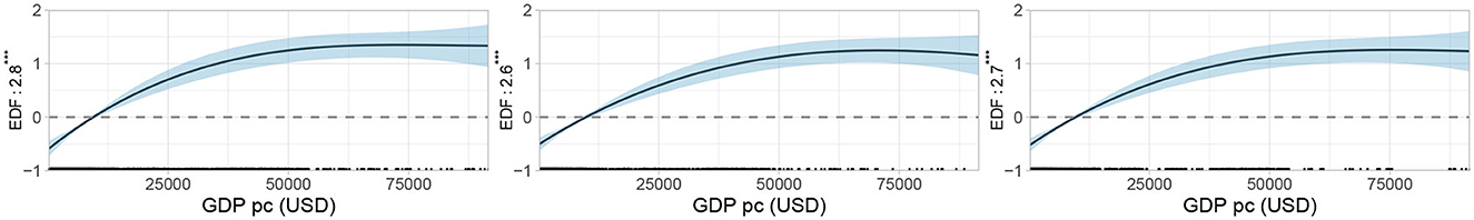
Figure 2. The estimate ĥ_{GDP pc (USD)}[GDP pc (USD)] results from the winning model M_6,1 specified under (2) and (12). The corresponding EDFs are reported along the y-axis. The ticks on the x-axis indicate the ranges of strong (dense ticks) and weak (sparse ticks) data support of the GDP pc (USD) variable.

5.1.2 Institutions

In all cases models with credit growth are more relevant than the models with M2 growth. GDP growth does better than GDP pc in 10 out of 12 cases. The freedom status variable bears also empirical relevance. However, these results are derived from a reduced sample size of 26 countries and a period from 2000 to 2012. The winning model is M_{16, 2} which features civil liberties next to credit growth and GDP pc. Due to the full-sample availability of civil liberties, we refitted the winning model on the full sample. The results are as follows: In the winning model all variables show evidence of a weak linear relationship with log inflation. In particular, credit growth (Figure 3) affects log inflation in a linear way. However, after the GFC, as indicated by missing asterisks of the EDFs, it cannot be told if the effect differs from zero. Estimated across the entire time span, the transition from no civil liberties to higher civil liberties is associated with an increasing impact on log inflation (0.01^* at most across levels). However, before the crisis, this effect was positive (0.12 at most) and turned negative afterwards (−0.2^* at most). GDP pc exerts a significant negative effect (−0.00001^***) across the entire period.

FIGURE 3

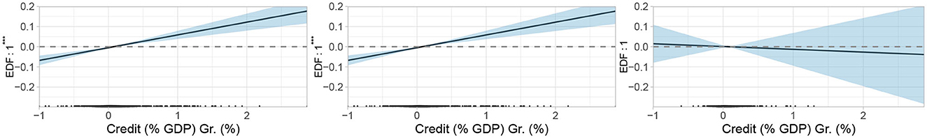
Figure 3. The estimate ĥ_{Credit (%GDP) Gr.(%)}[Credit (%GDP) Gr.(%)] results from the winning model M_16,2 specified under (2) and (12). The corresponding EDFs are reported along the y-axis. The ticks on the x-axis indicate the ranges of strong (dense ticks) and weak (sparse ticks) data support of the Credit (% GDP) Gr. (%) variable.

5.1.3 Monetary policy strategies

Models including exchange-rate arrangements (ERA) do better than those with inflation targeting. Credit growth and M2 growth do equally well in terms of empirical relevance, whereas GDP growth outperforms GDP pc in four out of four cases. M_{3, 3} is the winning model. According to it, ERA are important next to credit and GDP growth. The transition from a situation with no legal tender, actually a fixed-exchange-rate regime, to managed floating leads to a rise in log inflation (0.052^*). This effect is slightly weaker (0.031) for a transition to a crawling-peg and weakest for the transition to free-floating (0.002). No structural changes could be estimated for ERA due to singularities. Credit growth displays a positive linear relationship with log inflation (Figure 4). This holds before the crisis but vanishes after that, although estimated with high uncertainty. GDP growth also exhibits a linear effect (1.059^***), which has slightly strengthened after the crisis (1.439^***).

FIGURE 4

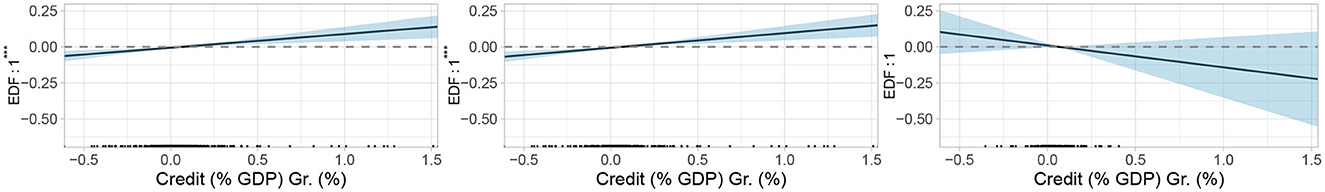
Figure 4. The estimate ĥ_{Credit (%GDP) Gr.(%)}[Credit (%GDP) Gr.(%)] results from the winning model M_3,3 specified under (2) and (12). The corresponding EDFs are reported along the y-axis. The ticks on the x-axis indicate the ranges of strong (dense ticks) and weak (sparse ticks) data support of the Credit (% GDP) Gr. (%) variable.

5.1.4 Public finance

Models with M2 growth do better than those with credit growth in seven out of eight comparisons. Models with GDP pc turn out to be better than the models that include GDP growth. Debt denomination [Denom. (%)] plays a dominant role while the maturity structure (Matur.) is less relevant. M_{14, 4} is the winner. Figure 5 summarizes the estimations which exhibit some non-linearities. It includes M2 growth, GDP pc and debt denomination. M2 growth exhibits a positive linear link with log inflation. In contrast, GDP pc (USD) reveals a clear non-linear link (Figure 5D). While the effect varies somehow below a threshold of 10,000 USD, it strongly increases beyond this income level. This pattern arises after the crisis (Figure 5F). Debt denomination exhibits a cubic association with log inflation over the entire period (Figure 5G). Beyond a share of public and publicly guaranteed external long-term debt denominated in a foreign currency of 20%, a further issuance reduces log inflation. The comparison between the pre-crisis period summarized in Figure 5H with the post-crisis period (Figure 5I), shows a clear break. Since then, increasing the share of foreign-currency debt linearly boosts log inflation. Due to data availability, this evidence is obtained for observations of low and middle-income countries where an effect may be more likely than in advanced countries. However, the results after the crisis contrast with theoretical predictions from the time-inconsistency literature. One possible explanation is that the more debt is issued in a form that protects investors from unexpected inflation, the higher the level of inflation required to reduce the inflation-sensitive part of the debt.

FIGURE 5

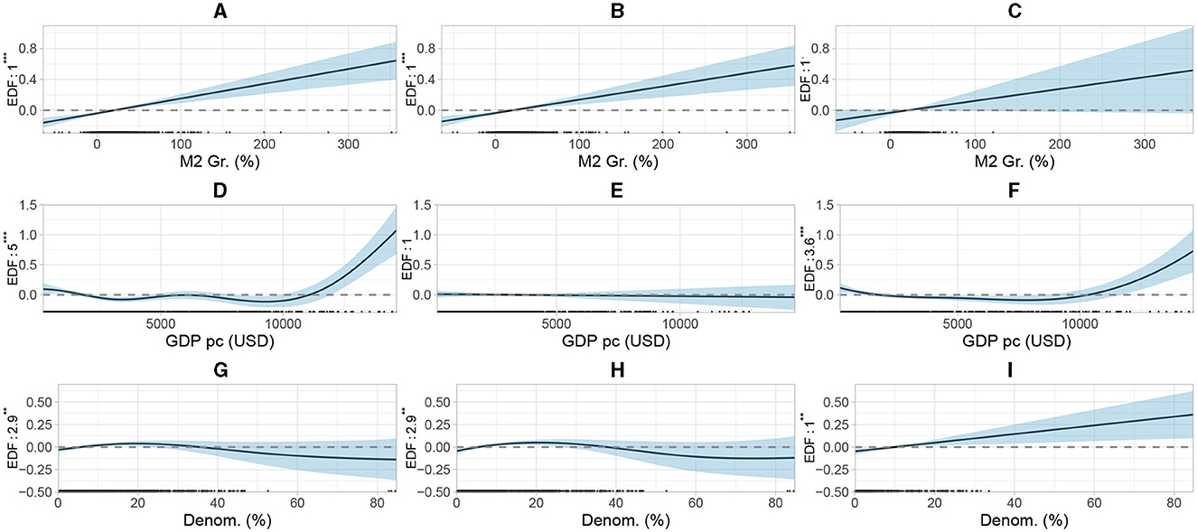
Figure 5. The three variables displayed result from the winning model M_{14, 4} specified under (2) and (12). The corresponding EDFs are reported along the y-axis. The ticks on the x-axis indicate the ranges of strong (dense ticks) and weak (sparse ticks) data support of the variables. ^*** indicates significance at the 0.1% level, ^** indicates significance at the 1% level, ^· indicates significance at the 10% level.

5.1.5 Globalization and technology

Models with GDP growth are superior to models that exhibit GDP pc in eight out of nine comparisons. Credit growth stands out in comparison with M2 growth in eight out of eight cases. The winning model is M_{20, 5} which features information and communication technology capital over the total capital stock (ICT Capital) next to credit and GDP growth. When ICT Capital is increased by one unit, log inflation rises by 4.088^*** c.p. on average (~4.1% increase in inflation). The effect weakens when separated into the pre-crisis (2.537^***) and the post-crisis (2.748^***) era. As illustrated in Figure 6 credit growth reveals a linear link with log inflation over the whole sample period and in the pre-crisis period but disappears subsequently. In contrast, while GDP growth hardly affected log inflation before the crisis (0.123), it has boosted inflation (1.581^***) thereafter, leading to an inflation rising relationship over the whole period (0.083^***).

FIGURE 6

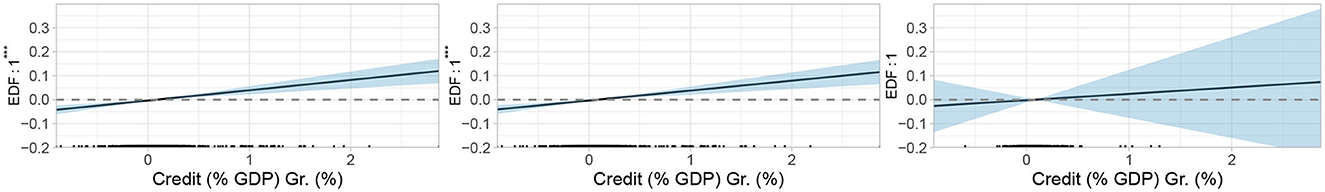
Figure 6. The estimate ĥ_{Credit (%GDP) Gr.(%)}[Credit (%GDP) Gr.(%)] results from the winning model M_{20, 5} specified under (2) and (12). The corresponding EDFs are reported along the y-axis. The ticks on the x-axis indicate the ranges of strong (dense ticks) and weak (sparse ticks) data support of the Credit (% GDP) Gr. (%) variable.

5.1.6 Demography

AMMs with credit growth fare better than those with M2 growth in three out of four cases. This also holds for the models featuring the share of the population older than or equal to 65 [Age 65 (%)] compared to those exhibiting the share of population older than or equal to 75. Models that include GDP pc are superior to the models with GDP growth in three out of four cases. M_{4, 6} exhibits the variable combination that best explains a relationship between demography and log inflation. It includes Age 65 (%) next to credit growth and GDP pc. Age 65 (%) exerts a significant (at all levels) negative effect on log inflation. If this share increases by 1% point, log inflation decreases on average by 0.039^***. This effect is of similar magnitude before the crisis (−0.032^***) but weakens afterwards (−0.022^***). From Figure 7 which displays the non-linear estimates of GDP pc, we can infer a similar non-linearity over the whole sample period as for GDP pc in the winning model M_{6, 1} illustrated in Figure 2. However, in contrast to M_{6, 1}, where the non-linearity holds up in all three (sub)periods, the effect changes from quadratic before the crisis to linear after the crisis. Note that we observe higher values of GDP pc after the crisis than before. Credit growth exhibits a positive linear association (0.023^*) across the whole sample. Before the crisis the effect is similar to the overall observation (0.025^***) but strengthens (0.085^***) after that.

FIGURE 7

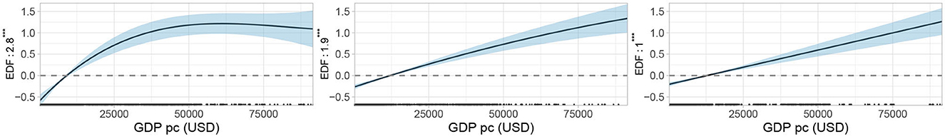
Figure 7. The estimate ĥ_{GDP pc (USD)}[GDP pc (USD)] results from the winning model M_{4, 6} specified under (2) and (12). The corresponding EDFs are reported along the y-axis. The ticks on the x-axis indicate the ranges of strong (dense ticks) and weak (sparse ticks) data support of the GDP pc (USD) variable.

5.1.7 Natural resources

In three out of four comparisons, AMMs that include credit growth instead of M2 growth yield a better result. Models with GDP pc are superior to those that contain GDP growth in two out of three cases. M_{12, 7} results as the winning model. It is composed of credit growth, GDP pc, and the interaction of energy prices with energy rents. From Figure 8 we can infer non-linear relationships. An acceleration in credit growth in the range between 0 and 150% (Figure 8A) pushes log inflation non-linearly. The effect is positive and linear before the crisis (Figure 8B) but becomes negative and non-linear in the post-crisis period (Figure 8C). Turning to GDP pc (Figures 8D–F), the relationship with log inflation is again similar to Figure 2. It is cubic throughout. Figures 8G–I illustrate the bivariate interaction effects between energy prices and energy rents using contour plots. They show the joint relationship between energy prices on the x-axis, energy rents on the y-axis, and log inflation. The passage from a blue to a red area denotes mounting inflationary pressure. Conversely, the passage from a red to a blue area indicates a decrease in inflation. The black contour (iso-effect value) lines indicate the strength of the effects which can only be interpreted on a relative scale, as discussed at the beginning of this section. Along the same iso-effect line the interaction effect does not change. From Figure 8G, a non-linear interaction effect between energy prices and rents can be inferred. When energy prices are below 75 USD while rents are high (above 25), the strongest impact on log inflation arises from an increase in energy prices. The effect from rising energy prices beyond 75 USD is still positive but weakens sharply. When energy rents hover below 25, an energy price increase still boosts log inflation, but by a much smaller magnitude than when rents are high. In the pre-crisis period, the relationship remains non-linear (Figure 8H). The post-crisis still exhibits a non-linear interaction as long as energy prices are below 50 USD, but disappears beyond this level. While an increase in energy prices still leads to more log inflation, a change in energy rents leaves log inflation unaffected for any value of energy prices above 50 USD (c.p.).

FIGURE 8

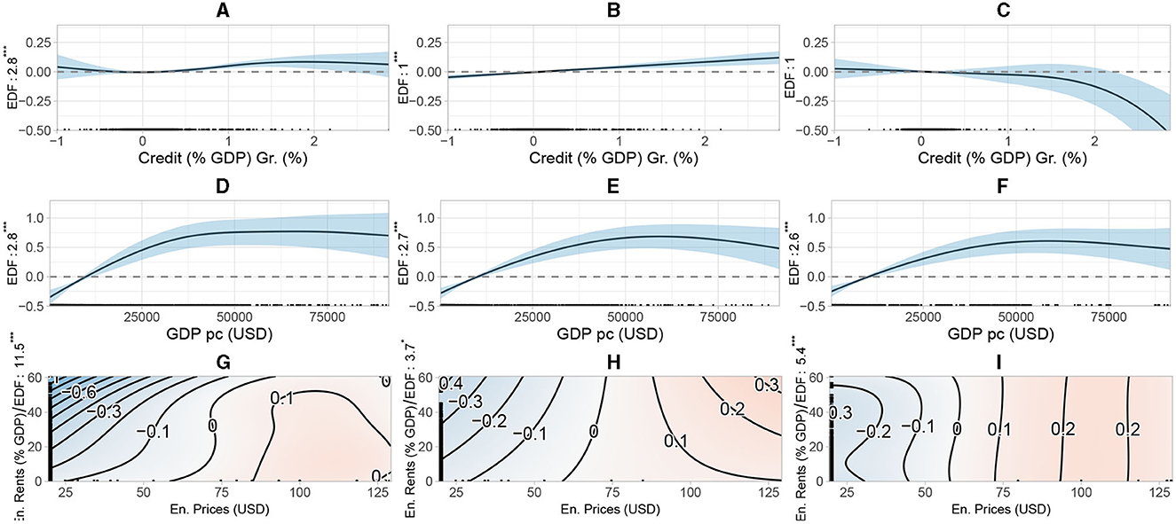
Figure 8. The three variables displayed result from the winning model M_{12, 7} specified under (2) and (12). The corresponding EDFs are reported along the y-axis. The ticks on the x-axis indicate the ranges of strong (dense ticks) and weak (sparse ticks) data support of the variables.

5.1.8 Past inflation

AMMs that feature M2 growth strictly outperform AMMs that exhibit credit growth. No clear picture emerges from the comparison of AMMs that include GDP pc with models that include GDP growth. The winning model is M_{2, 8} and includes past inflation together with M2 growth and GDP pc. There is evidence of a positive linear effect (0.001^***) from past inflation estimated over the whole sample period. While the relationship did not change, the strength of the effect increased somewhat since the crisis (0.011^***) compared with the preceding period (0.001^***). As seen in the left panel of Figure 9, there is a quadratic relationship between M2 growth and log inflation in the whole sample, but with evidence for a linear relationship in the region with the most data support. The uneven distribution of the data should limit the interpretation of the effects in areas without any data support. An acceleration of M2 growth below a level of 100% raises inflation. Beyond 100%, the impact becomes highly uncertain. In contrast, before the crisis the center panel suggests that M2 Gr.(%) impacted log inflation linearly. After the crisis, the effect strengthened slightly. In contrast, GDP pc exhibits a positive and linear effect over the whole period (0.00002^***), before (0.00002^***) and after the crisis (0.00002^***).

FIGURE 9

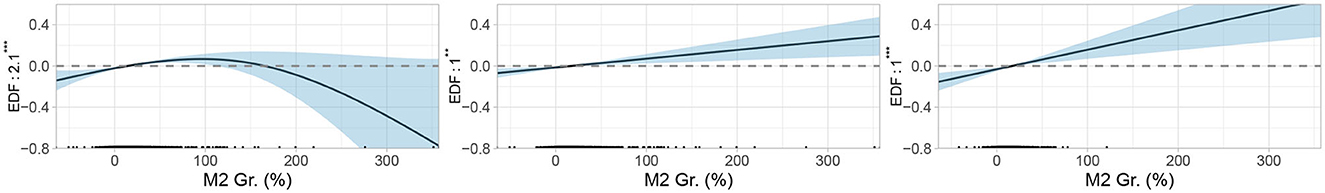
Figure 9. The estimate ĥ_{M2 Gr. (%)}[M2 Gr. (%)] results from the winning model M_{2, 8} specified under (2) and (12). The corresponding EDFs are reported along the y-axis. The ticks on the x-axis indicate the ranges of strong (dense ticks) and weak (sparse ticks) data support of the M2 Gr. (%) variable. ^*** indicates significance at the 0.1% level, ^** indicates significance at the 1% level.

We do not explicitly examine how people form their inflation expectations. However, the importance of past inflation suggests the existence of (at least a share of) “adaptive expectations users” in practice.

5.2 Second stage selection

In ${\mathcal{S}}_{fir}$, discussed in Section 5.1, we derived the winning model for each economic theory. In this subsection, we discuss the derivation of the overall winning model, M^**. This required a second stage selection because the winning model of the first stage for four of the theories examined was obtained from a lower number of countries and a reduced period. This applies to theories associated with institutions, monetary policy strategies, public finance, and globalization and technology (${\mathcal{M}}_2$, ${\mathcal{M}}_3$,${\mathcal{M}}_4$ and ${\mathcal{M}}_5$). Their Likelihood and thus their cAICs cannot be directly compared with the AMMs from the other theories—${\mathcal{M}}_1$, ${\mathcal{M}}_6$, ${\mathcal{M}}_7$, ${\mathcal{M}}_8$—and the AMM selected by the boosting algorithm, M_B. However, since some AMMs comprised by ${\mathcal{M}}_2$, ${\mathcal{M}}_3$, ${\mathcal{M}}_4$ and ${\mathcal{M}}_5$ contain M_{j, l} associated with predictor sets A_{j, l} that are also available for the full sample, these M_{j, l} can be refitted on the full sample, in case they were selected during ${\mathcal{S}}_{fir}$. This is the case for ${\mathcal{M}}_2^{*}$. As a result, ${\mathcal{M}}_2^{*}$ has been refitted on the full sample and was added to the comparison of the AMMs that were already estimated during the first stage comparison (i.e., M_{6, 1}, M_{20, 5}, M_{4, 6} and M_{12, 7}). We next present M_B and compare its cAIC against the cAIC of the first-stage winners.

5.2.1 AMM selected by the boosting algorithm

The boosting algorithm selected the set of predictors A_B which can be inferred from the last subsection of Table A2 exhibited in the Appendix. This subsection also includes separating all selected predictors into disjoint subsets, informing which predictors were modeled (non-)linearly and/or through a bivariate interaction. For the boosting algorithm we added more predictors to those exhibited in the AMMs presented in Section 5.1. These additional variables are domestic credit level by the financial sector in percent of GDP [Credit Fin. (% GDP)] and its growth rate [Credit Fin. (% GDP) Gr. (%)]. The remaining additional variables are M2 (% GDP), Credit (% GDP), Debt (% GDP), En. Price Gr. (%), En. Rents Gr. (%), GDP (USD) and GDP pc Gr. (%).

Figures 10–12 present the non-linear effect estimates included in M_B. Past inflation (Figures 10A–C) suggests such a pattern across the whole sample but with high uncertainty when assessed over the whole sample period. However, in the range where most observations lie (< 250%), the relationship is linear with a positive slope. The same observation holds for the pre- and post-crisis period. The bivariate interaction of energy prices and rents (Figure 10D) confirms the results from the estimation of M_12;7 illustrated in Figure 8, at least over the entire sample. In the pre-crisis period the interplay between energy prices and rents weakens (Figure 10E). An increase in energy prices beyond 75 USD would lower log inflation, irrespective of the value of energy rents. Below energy prices of 75 USD a rise in energy prices would increase log inflation and still for any level of energy rents. On the other hand, if energy rents rise, there is hardly any effect on log inflation, regardless of the level of energy prices. Finally, in the post-crisis era (Figure 10F), the impact of the interaction of energy prices and rents vanishes completely. When interpreting these results it has to be kept in mind that M_B estimates the univariate effects of energy prices and rents in contrast to M_{12, 7} which estimates their interaction.

FIGURE 10

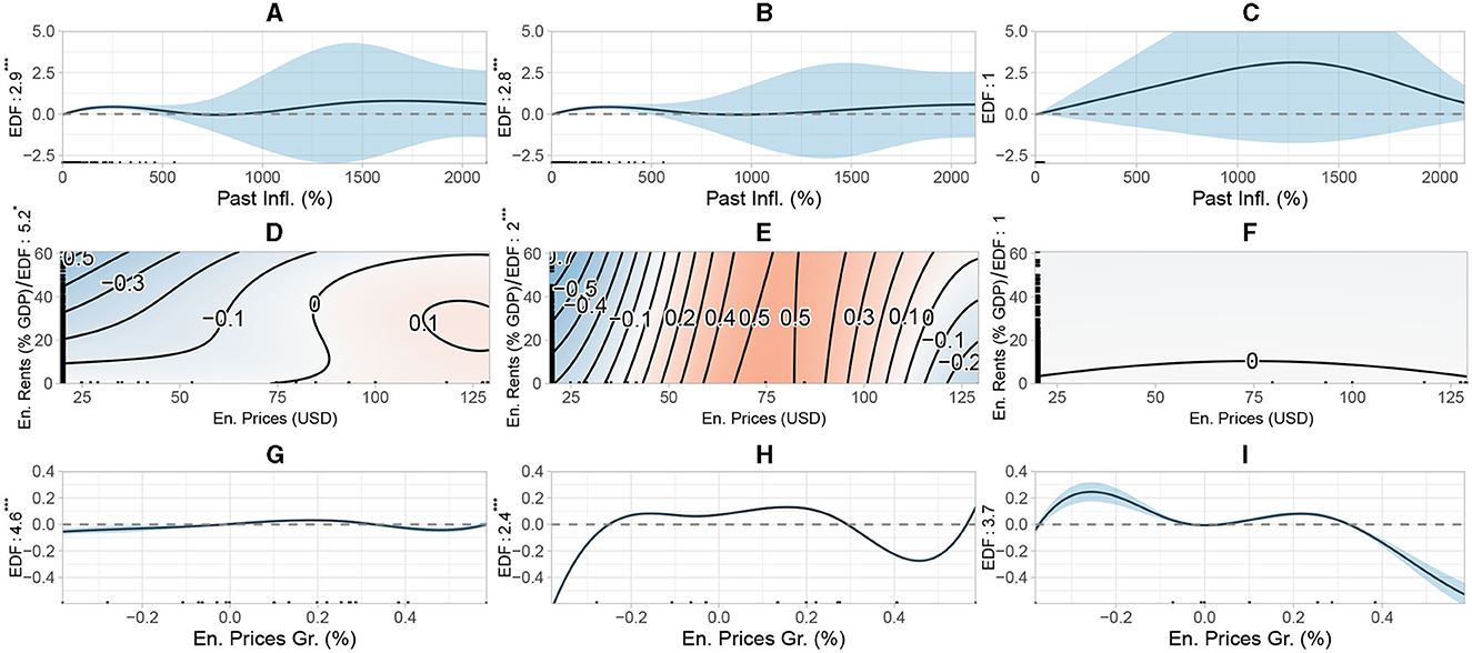
Figure 10. The first out of three plots that displays the estimated non-linear effects from M_B.

Figures 10G–I display the results of energy price growth. Over the whole sample, the relationship is highly non-linear (Figure 10G). For a growth rate of energy prices below 20% a rise in the growth rate increases log inflation. Beyond a growth rate of 20% a further energy price rise has an inflation abating effect, followed again by an acceleration above 50%. The evidence for the pre-crisis period can be seen in Figure 10H and in the post-crisis period in Figure 10I. Note that the variation for the energy price variable (and its growth) results exclusively from the time variation and not from the cross-country variation, as we have identical energy prices for each country in the estimation. The resulting uneven distribution of the data weakens the reliability of the effects in areas without any data support.

Figure 11 summarizes the results of financial openness, energy prices and credit. As long as values of financial openness hover below 0.6, an increase in openness lowers log inflation but increases it beyond this threshold (Figure 11A). This pattern also holds before the crisis (Figure 11B) but turns linear (Figure 11C) after the crisis. Energy prices show again a strong non-linear relationship (Figure 11D). Below 80 USD, a rise in energy prices is conducive to inflation, although subject to high uncertainty. Afterward, the effect turns negative. The evidence preceding the crisis (Figure 11E) suggests that energy prices were associated with lower inflation, especially beyond 80 USD. However, this changed dramatically after the crisis (Figure 11F) where energy price boosts below 80 USD are linked with continuously higher log inflation and stagnation afterward. For credit the relationship is also non-linear but positive and strong for values below 50 over the whole sample (Figure 11G). When separating into the pre- (Figure 11H) and the post-crisis period (Figure 11I), the effect does not differ from zero.

FIGURE 11

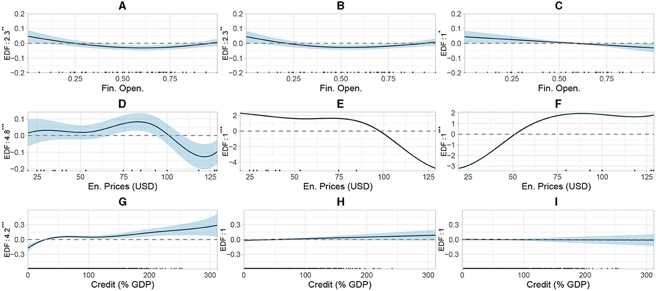
Figure 11. The second out of three plots that displays the estimated non-linear effects from M_B.

The last non-linear effects comprised by M_B are shown in Figure 12 and relate to the output gap whose pattern suggests a cubic relationship with log inflation. Log inflation is boosted by a widening gap between −5 and 20% and followed by a negative effect (although subject to increasing uncertainty). This pattern holds over the whole sample and in the period preceding the crisis. However, after the crisis, the relationship has changed, becoming negative for output gap values below −5% and positive after that.

FIGURE 12

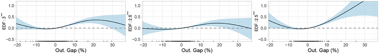
Figure 12. The third out of three plots that displays the estimated non-linear effects from M_B.

Finally, all linearly estimated effects of M_B are insignificant at the 10% level. One exception is M2 growth (0.0005^*) whose impact weakens before the crisis (0.0004) but turns stronger (0.003^***) after the crisis. The second exception is trade openness which exhibits a negative impact on log inflation (−0.001^*) across the whole sample but turns insignificant when separated into a pre- and post-crisis effect.

5.2.2 Overall winner

As seen in Tables A1, A2 the comparison among theory-based winning models yields M_{12, 7} as the best model.

The estimation equation for M_{12, 7} is given by

$\begin{array}{ll}{y}_{i,t}={\beta }_0+{\eta }_{i,t}+Z_{i,t}{b}_i+{ϵ}_{i,t},& (13)\end{array}$

where

$\begin{array}{ll}{\eta }_{i,t}=h_{Credit}(Credit)+h_{GDPpc}(GDPpc)+f_{(Credit,GDPpc)}(Credit,GDPpc)& (14)\end{array}$

and b_i is a vector of fixed country effects. Table 1 summarizes the results of this model. Its predictor η_{i, t} consists of three non-linear terms only which motivates conducting three F-tests, one for each non-linear term. Each test is significant at all common significance levels.

TABLE 1

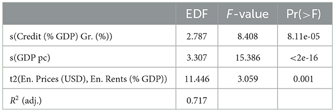
Table 1. Summary of the estimates of the spline function of the theory-based winning model M_{12, 7}.

However, the lowest cAIC overall is exhibited by M_B. Since both AMMs feature variables associated with natural resources, we conclude that these variables play a key role in the inflation (disinflation) process. In particular, the interaction of prices and rents of natural resources exhibited in M_B and M_{12, 7} seems to have particularly high explanatory power. The empirical relevance is higher when energy rents and prices interact than when they enter as two separate univariate terms. Moreover, their interacting effects are highly non-linear. The boosting algorithm supports this interaction and shows the importance of energy prices and their growth rate as additional univariate drivers of inflation. Finally, we computed the cAIC for models that do not contain any economic variable at all (that is, they exhibit no effects other than for time and country-level) and found a substantially higher cAIC for these models compared to every other model included in the first and second stage selection. Consequently, it can be inferred that model compilation based on economic theory significantly improves the goodness-of-fit.

Summarizing the evidence of the pairwise comparisons on a meta-level yields that credit growth outperforms M2 growth and GDP pc outperforms GDP growth.

6 Conclusions

We contribute to the literature on what determines inflation and how by estimating a large quantity of macro, institutional and political models in a sample of 122 countries at different stages of development from 1997 to 2015.

From among the eight theories, the winning model includes energy prices whose importance has already been highlighted in previous work. However, we find that the most compelling determinant of inflation are not energy prices alone but their interplay with energy rents which exhibits a strong non-linear association with inflation. The atheoretical boosting algorithm confirms the importance of the interplay of energy prices with energy rents. It outperforms all theoretically motivated models in terms of explanatory power and suggests, in line with previous analyses, a particular role for energy prices. Energy rents by themselves do not seem to be as important.

The results have a bearing on monetary policy. The empirical importance of energy prices (and rents) has implications for when and how central banks need to respond to oil price shocks. Another challenge to monetary policy-making arises from the link between past and current inflation in a low-inflation environment. One way to lift inflation has been the stimulus of credit creation. However, there is little evidence that this policy was successful. It cannot be excluded that it even backfired. A promising tool to boost inflation is higher GDP per capita level. This suggests that economic policies geared toward growth should be more promising than monetary policies aimed at enhancing credit growth. Another result relates to the output gap. While in monetary theory and policy it is considered a key variable in the determination of inflation, it plays a minor role compared to GDP per capita.

We used AMMs to represent inflation rates. AMMs proved to be an effective technique for this purpose for a variety of reasons. First, they allow for a smooth integration of model complexities, making it easier to model non-linearities, which represents one focal objective of this paper. Second, AMMs allow for a straightforward “ceteris paribus” interpretation, which is beneficial to the analysis of the relationship between predictors and inflation. Third, AMMs enable researchers to make model comparisons using information criteria, simplifying the model selection process.

Data availability statement

The original contributions presented in the study are included in the article/Supplementary material, further inquiries can be directed to the corresponding author.

Author contributions

PB: idea, data collection and processing, development and implementation of the statistical strategy, model estimation, coding, writing of the methodology and results section, and figures and tables. ER: idea, macroeconomic interpretation, writing of the economic theory sections, and proof reading. AV: idea, data collection and processing, development of the statistical strategy, and proof reading. All authors contributed to the article and approved the submitted version.

Funding

Open access funding provided by ETH Zurich.

Acknowledgments

We thank all participating referees, Jan-Egbert Sturm, David Rügamer, and the participants of the Swiss National Bank Brown Bag Workshop for their helpful comments and suggestions.

Conflict of interest

The authors declare that the research was conducted in the absence of any commercial or financial relationships that could be construed as a potential conflict of interest.

Publisher's note

All claims expressed in this article are solely those of the authors and do not necessarily represent those of their affiliated organizations, or those of the publisher, the editors and the reviewers. Any product that may be evaluated in this article, or claim that may be made by its manufacturer, is not guaranteed or endorsed by the publisher.

Author disclaimer

The views expressed in this article are those of the author(s) and do not necessarily reflect those of the Swiss National Bank. A preprint of this paper appeared on Arxiv and in the SNB Working Paper Series.

Supplementary material

The Supplementary Material for this article can be found online at: https://www.frontiersin.org/articles/10.3389/fams.2023.1070857/full#supplementary-material

Footnotes

1. ^Blanchard [1] and Borio [2] have even put into question economists' knowledge of its process.

2. ^See Baumann et al. [6] for details.

3. ^See, e.g., Degruttola et al. [8] and Pearson et al. [9].

4. ^See Saefken et al. [17] and Greven and Kneib [20].

5. ^When x corresponds to the EDF or the linear effect, x^*** corresponds to significance at the 0.1% level, x^** at the 1% level, x^* at the 5% level, x^· at the 10% level and no asterisks indicates no significance at the 10% level.

References

1. Blanchard OJ. The US Phillips Curve: Back to the 60s? Tech. Rep. PB16-1. Washington, DC: Peterson Institute for International Economics (2016).

Google Scholar

2. Borio C. Through the Looking Glass. London: Bank for International Settlements; OMFIF City Lecture (2017).

Google Scholar

3. Rogoff KS. Globalization and Global Disinflation. Jackson Hole, WY: Federal Reserve Bank of Kansas City Economic Review (2003). p. 45–78.

Google Scholar

4. Baumann PFM, Rossi E, Volkmann A. What Drives Inflation and How? Evidence from Additive Mixed Models Selected by cAIC. In: Swiss National Bank Working Paper Series. Zurich: Swiss National Bank (2021) p. 12

Google Scholar

5. Honaker J, King G, Blackwell M. Amelia II: a program for missing data. J Stat Softw. (2011) 45:1–47. doi: 10.18637/jss.v045.i07

CrossRef Full Text | Google Scholar

6. Baumann PFM, Schomaker M, Rossi E. Estimating the effect of central bank independence on inflation using longitudinal targeted maximum likelihood estimation. J Caus Infer. (2021) 9:109–46. doi: 10.1515/jci-2020-0016

CrossRef Full Text | Google Scholar

7. Hastie T, Tibshirani R. Varying-coefficient models. J R Stat Soc Ser B. (1993) 55:757–79. doi: 10.1111/j.2517-6161.1993.tb01939.x

CrossRef Full Text | Google Scholar

8. Degruttola V, Lange N, Dafni U. Modeling the progression of HIV infection. J Am Stat Assoc. (1991) 86:569–77. doi: 10.1080/01621459.1991.10475081

CrossRef Full Text | Google Scholar

9. Pearson JD, Morrell CH, Landis PK, Carter HB, Brant LJ. Mixed-effects regression models for studying the natural history of prostate disease. Stat Med. (1994) 13:587–601. doi: 10.1002/sim.4780130520

PubMed Abstract | CrossRef Full Text | Google Scholar

10. Mundlak Y. On the pooling of time series and cross section data. Econometrica. (1978) 46:69–85. doi: 10.2307/1913646

CrossRef Full Text | Google Scholar

11. Eilers PH, Marx BD. Flexible smoothing with B-splines and penalties. Stat Sci. (1996) 11:89–102. doi: 10.1214/ss/1038425655

CrossRef Full Text | Google Scholar

12. Wood SN. Fast stable restricted maximum likelihood and marginal likelihood estimation of semiparametric generalized linear models. J R Stat Soc B. (2011) 73:3–36. doi: 10.1111/j.1467-9868.2010.00749.x

CrossRef Full Text | Google Scholar

13. Wood S, Scheipl F. gamm4: Generalized Additive Mixed Models Using ‘mgcv' and ‘lme4'. R package version 0.2-5 (2017). Available online at: https://CRAN.R-project.org/package=gamm4

Google Scholar

14. R Core Team. R: A Language and Environment for Statistical Computing. Vienna (2020).

Google Scholar

15. Karlsson S, Mazur S, Nguyen H. Vector autoregression models with skewness and heavy tails. J Econ Dyn Control. (2023) 146:104580. doi: 10.1016/j.jedc.2022.104580

CrossRef Full Text | Google Scholar

16. Akaike H. Information theory and an extension of the maximum likelihood principle. In:Petrov BN, Csaki F, editors. Selected Papers of Hirotugu Akaike. Springer Series in Statistics. New York, NY: Springer (1973).

Google Scholar

17. Säfken B, Rügamer D, Kneib T, Greven S. Conditional model selection in mixed-effects models with cAIC4. J Stat Softw. (2021) 99:1–30. doi: 10.18637/jss.v099.i08

CrossRef Full Text | Google Scholar

18. Vaida F, Blanchard S. Conditional Akaike information for mixed-effects models. Biometrika. (2005) 92:351–70. doi: 10.1093/biomet/92.2.351

CrossRef Full Text | Google Scholar

19. Liang H, Wu H, Zou G. A note on conditional AIC for linear mixed-effects models. Biometrika. (2008) 95:773–8. doi: 10.1093/biomet/asn023

PubMed Abstract | CrossRef Full Text | Google Scholar

20. Greven S, Kneib T. On the behaviour of marginal and conditional AIC in linear mixed models. Biometrika. (2010) 97:773–89. doi: 10.1093/biomet/asq042

CrossRef Full Text | Google Scholar

21. Saefken B, Ruegamer D, Sonja G, Kneib T. cAIC4: Conditional Akaike Information Criterion for lme4. Foundation for Open Access Statistics (2018).

Google Scholar

22. Bates D, Mächler M, Bolker B, Walker S. Fitting linear mixed-effects models using lme4. J Stat Softw. (2015) 67:1–48. doi: 10.18637/jss.v067.i01

CrossRef Full Text | Google Scholar

23. Overholser R, Xu R. Effective degrees of freedom and its application to conditional AIC for linear mixed-effects models with correlated error structures. J Multivar Anal. (2014) 132:160–70. doi: 10.1016/j.jmva.2014.08.004

PubMed Abstract | CrossRef Full Text | Google Scholar

24. Verbyla AP, Cullis BR, Kenward MG, Welham SJ. The analysis of designed experiments and longitudinal data by using smoothing splines. J R Stat Soc Ser C. (1999) 48:269–311. doi: 10.1111/1467-9876.00154

CrossRef Full Text | Google Scholar

25. Eilers PHC, Brian DM, Maria D. Twenty years of P-splines. Stat Operat Res Transact. (2015) 39:149–86.

Google Scholar

26. Currie ID, Durban M, Eilers PHC. Generalized linear array models with applications to multidimensional smoothing. J R Stat Soc Ser B. (2006) 68:259–80. doi: 10.1111/j.1467-9868.2006.00543.x

CrossRef Full Text | Google Scholar

27. Bühlmann P, Hothorn T. Boosting algorithms: regularization, prediction and model fitting. Stat Sci. (2007) 22:477–505. doi: 10.1214/07-STS242

CrossRef Full Text | Google Scholar

28. Hofner B, Mayr A, Robinzonov N, Schmid M. Model-based boosting in R: a hands-on tutorial using the R package mboost. Comput Stat. (2014) 29:3–35. doi: 10.1007/s00180-012-0382-5

CrossRef Full Text | Google Scholar

29. Hothorn T, Buehlmann P, Kneib T, Schmid M, Hofner B. mboost: Model-Based Boosting. R package version 2.9-1 (2018). Available online at: https://CRAN.R-project.org/package=mboost

Google Scholar

30. Wood SN. On p-values for smooth components of an extended generalized additive model. Biometrika. (2013) 100: 221–8. doi: 10.1093/biomet/ass048

CrossRef Full Text | Google Scholar

31. Wood SN. Generalized Additive Models: An Introduction With R. 2nd ed. Boca Raton, FL: Chapman and Hall/CRC (2017).

Google Scholar