 Anthony O'Hare
94% of researchers rate our articles as excellent or good
Learn more about the work of our research integrity team to safeguard the quality of each article we publish.
Find out more
METHODS article
Front. Appl. Math. Stat. , 02 February 2023
Sec. Mathematical Biology
Volume 9 - 2023 | https://doi.org/10.3389/fams.2023.1058273
This article is part of the Research Topic Insights in Mathematical Biology 2022 View all 4 articles
The drive to maximize food production in a sustainable manner is a paramount concern for farmers and governments. The aim of food producers is to maximize their production yield employing actions such as application of fertilizer or pesticide they believe help to achieve this aim. However, farms do not exist in isolation, but rather share a landscape with neighbors forming networks where any action taken by any one farmer affects their neighbors who are forced to take mitigating actions creating a complicated set of interactions. Understanding these [non-]cooperative interactions and their effect on the shared ecosystem is important to develop food security strategies while protecting the environment and allowing farmers to make a living. We introduce a simple competitive agent based model in which agents produce food that is sold at a fixed price (we ignore market dynamics and do not include explicit punishment on any agent). We analyzed agent's profits in several simple scenarios allowing us to identify the most advantageous set of actions for maximizing the yield (and thus profit) for each farmer. We show that the effect of the structure of the network on each farm has implications on the actions taken by agents. These results have implications for the understanding of the effects of farming practices on the environment and how different levels of cooperation between farmers, taking into account the local terrain, can be used to incentivise producers to minimise the effects on the environment while maximizing yields.
With an ever increasing global population, the need to maximize food production in a sustainable manner is a paramount driver for producers throughout the world. The global food system is complex with many interconnected and interdependent parts. Much research is being done in individual aspects of this complex system [1] but this assumes that each facet of the food system can be separated into individual isolated units with less research on how these facets interact [2].
The economic goal of any food producer is to either maximize their crop yield or minimise the growing time so as to get their produce to market as quickly as possible, thereby gaining a premium. However, farms share a landscape with neighbors forming complex dynamic interactions where the actions of any one farmer affects their neighbors who are compelled to take mitigating actions of their own creating a complicated set of interactions that have an impact on the landscape and ecosystem [3].
To reduce the impact of agricultural land use on the landscape, ecosystem, and biodiversity requires modeling of the interdependencies of farmers, wildlife, climate, soil at the landscape scale and the decisions humans make within this system [4]. Several research programs exists that attempt to address these complex interactions at the landscape level [5–9] and there are many review papers [10–12] on the research on land use and its impact on climate change [13–15], health [16], diversity [17, 18], the impact of different management policies on food production and biodiversity [19–21], and the impact of externalities [22] but relatively fewer at the farm level where decisions on land use and management are made [2]. A further complication in modeling landscapes is that the landscape interaction is highly correlated with any resident population or farmer-industrialist occupation [23–25].
Agent Based Models (ABM) are a computational framework that models autonomous individuals and their interactions and are routinely used in land use and land cover models [26–29]. They can easily accommodate game theory in accounting for decision making of the agents in a flexible manner [30] and are suitable for studying complex socio-ecological systems [30–33].
Traditional economic models assumes that agents have complete and perfect information on the other agents in the system. Current models incorporate the notion of bounded rationality, that rational decision makers may make sub-optimal decisions in some circumstances [34]. Humans do not complete a cost-benefit analysis to calculate their optimal position but make decisions that produce a satisfactory solution, a process known as satisficing. Satisficing has been implemented in ABMs [35].
A mathematical analysis of the effects of different management actions that may be employed on farms is required at a regional level to understand the possible feedback mechanisms that exist. A shared landscape provides a mechanism for the actions of a farmer to affect (positively or negatively) their neighbors. Systems such are these are dynamical in nature as each farmer can modify the set of actions they choose to make at any time during (or between) a growing season to maximize their crop yields. In reality, there are limits to what farmers are permitted to do in terms of application of pesticides etc. but other management strategies make the system dynamic. Understanding these [non-]cooperative actions available to farmers and their affect on the shared ecosystem is important to develop food security strategies while protecting the environment and allowing farmers to make a living.
In this paper we look at the effect of competitive behavior between individual food producers (farmers) based on simple economic principles in an agent-based framework that incorporates an agents' actions for maximizing their crop yield and the subsequent effects on their neighbors. The assumption is that farms are well established and are not able to change the produce they grow due to local conditions or topology. Traditional land use models mainly focus on dynamic decisions on how to use land rather than on the effect of long established land use patterns.
We model two types of farms in a very simplistic manner, 1) simple sigmoidal crop growth where farmers only harvest (realize a profit) at the end of the season, mimicking the production of cereal crops, and 2) a continuous growth model, mimicking the growth of animals that may be sold to realize profit at any time. We model farm inputs as being beneficial to similar farms, for example a crop farmer may use pesticides or fertilizers that are taken into the environment and shared at an ecosystem or regional level and prove beneficial to other crop farms. However, without modeling the exact mechanisms we assume that the input is detrimental to different farms, for example any wind blown excess from a crop farmer using pesticides would prove detrimental to farms such as fruit farms which require pollinating insects. Furthermore, we assume that the benefit or detriment decays with distance so the further apart farms are the less their effect on each other. This simplistic approach is enough to demonstrate the importance landscape plays in farming systems.
We create a toy model that incorporates the basics of food production and how farms producing different crops interact. The goal is illustrate how a system of food production behaves at a landscape level without specific detail of crops grown and how they interact.
Let us consider a system of food producers (in the language of ABM they are called agents or actors but we will refer to them here as farmers) growing food in a locally closed environment, i.e., there are no interactions with farms outside the system so we can ignore boundary effects. For simplicity, we will refer to the food produced as a crop (even if the farm rears animals for food). In such a closed system is reasonable to expect the crop management on one farm can impact on neighbors, for example, one can imagine that fertilizer or pesticide sprayed on one farm may be carried by the wind, or can runoff into watercourses to neighboring farms. The impact on neighboring farms can be either positive (for example, if both farms grow the same crop and windblown pesticides provide an, albeit small, positive benefit) or negative (reducing a neighbors ability to grow their crop, if, for example, pesticide use on one farm reduces fruit pollinator population).
The growth of each farmer's crop can be described as a function of the management actions employed by all farmers in the system, ui, j(t), as ψi(t, ui, j(t)). The subscript i refers to each farmer and j their neighbor; we note that ui = j(t) is the strategy employed by i to increase the yield of their crop and ui≠j(t) is the effect from a neighboring farm j. Profit can be realized by selling the crop at a unit price of pi(t), allowing each farmer to have a different conversion factor which may be realized by selling in different markets etc. In this paper we will have a constant p(t) for each crop type and further simplify this by setting p(t) = 1. The total turnover that a farmer can realize is thus given by the expression
where th is the harvest date and δth(t) is the Heaviside step function which is evaluated as 0 if t < th and 1 if t ≥ th so that a farmer cannot realize any profit until the crop is harvested. A farmer can monitor the growth of their crop throughout its growing season and so can decide to take an action to either increase growth or negate detrimental effects of their neighbors strategies at any time (subject to local laws etc).
The cost can be split into 2 parts; fixed costs such as the initial start-up cost (buying brood stock or seed) and the cost of managing the crop, for example the daily running costs of the farm and the costs of any management strategies employed. The running cost to each farmer i of producing their crop as
The profit for each farmer can now be defined as
We can clearly see that a farmer will obtain a profit if , i.e., they can sell their crop for more than it costs to produce. In this simple model, the ability of each farmer to produce food is a competition between the growth of their crops, ψi(t), and the strategies employed by their neighbors, uj(t).
We will ignore market forces for the remainder of this paper, assuming that the food produced is limited only by the environment on which they produce their food that the demand is such that we can make the simplifying assumption of pi(t) = 1 regardless of the crop grown.
Two simple growth models will be employed in this analysis; a linear model that may describe the growth of food production animals, particularly in the fattening stage, and a logistic model as it broadly describes the characteristic of little or no growth until a ‘harvestable' future time and thus no income can be derived until the crop is harvested. The implicit assumption here is that the crop doesn't spoil and can be stored until it is sold.
In the linear model case, the growth of the crop, planted or born at t0, at some time t > t0 is given by
Where α, β are the parameters of the linear equation and the summation term sums the interactions from the other farms integrated over the whole growing season from when the strategy was employed.
For the logistic growth model, the food production on farm i at time t is given by
Where the first term is simply a logistic growth model with a maximum output L, steepness k, and th when the crop is ready for harvesting, and the summation term describes the interactions with the other farms. The assumption is that the crop has little to no value until it is harvested and the time to harvest is short compared to its growing season. We also assume that the crop doesn't spoil once harvested.
We will use the following simple interaction term (over time and space) to define the effect of the jth farm on the ith as
Where Iij is the effect of the action employed on farm j on farm i, γ and ϕ scale the decay rates of the action over space and time respectively, τ is the time since the action was employed, rij is the distance between farms. To avoid multiplying by zero in the case when there is no interaction between farms (i.e., no farmer has performed any action) we add 1 to μij. This means a farmer may implement an action to increase their yield such as apply a pesticide or fertilizer and the effect will decay over time, while also affecting their neighbors positively, if they grow the same crop, or negatively, if they grow a different crop but the effect decays both in time and distance. We implicitly assume that the effect extends radially and uniformly from the source farm and do not include any directionality due to, for example, wind.
To solve our model (Equation 3) we will use two different types of farms, one using a crop that is described by a linear growth model with parameters α = 0.028 and β = 0.02 and another by a logistic growth model with parameters L = 5.8, k = 0.7, th = 150. We assume is that the crop has little to no value until it is harvested and the time to harvest is short compared to its growing season, thus the sharp curve from an almost zero saleable value to a significant one (decreasing this value, so that the harvest period is longer, doesn't appreciably change the output).
We give each farm containing a linear growth crop a an initial cost of 0.25 to model the purchase of seed or stock, and a daily fixed cost of 0.001 to model the continuous monitoring and management of the farm and an initial cost of 0.15 with a daily cost of 0.001 for a logistic growth crop. These costs are in units of local currency.
Farms that grow crops with a linear model apply some treatment on day 10 with a cost of 0.35 and farms that grow a logistic crop apply treatments on days 50 and 100 each with a cost of 0.25. We set the interaction between farms to ±0.3 which decay at a rate of and γ = 0.07, ϕ = 0.008 again in arbitrary units since the goal is to observe a general pattern rather than model a specific location. We do not impose any restrictions on the range of the interactions between farms allowing farms on either end of the network to interact, albeit with limited effect.
The model is run on three different farm networks on a square grid; circular, and linear with each farm equidistant from their nearest neighbor; and randomly.
We solve the model Equation 3 by calculating the growth of the crop (Equations 4, 5) each day over a period of 240 days. What we calculate is the profit a farmer would realize if they harvested and sold their crop on a particular day and a farmer may harvest and sell early to realize a profit sooner or to avoid potential losses due to negative interactions due to their neighbors management. We largely ignore this level of economics here and simply calculate the profit as a time-series.
When each farm within the model grows the same crop, farmers apply the same action and since the mutual interactions are all positive the strength of each farmer's action can be reduced with no loss of production value, and since each action has a cost, a saving can be made. In this case, a Nash equilibrium exists from the mutually beneficial interactions between farms and farmers cannot gain extra savings from an alternative strategy or alternative crop.
In a circular network where each farm is equidistant from their nearest neighbor, a symmetry exists when every farm produces the same crop. Here the sum of the inter-farm interactions of each farm are the same and so everyone gains the same profit. This symmetry is removed when there is a heterogeneity in the crops produced by each farm (the heterogeneity here is due to a new class of crop representative of livestock added to the network). The physical layout and profit are shown in Supplementary Figures S1, S2 where a distribution of profit can be seen due, solely, to the imbalance of the neighboring strategies.
No such symmetry exists when farms are laid out in a linear network. Some farms, particularly those in the center, have an equal number of neighbors on each side so gain more positive benefit in a homogeneous crop landscape and so have a greater crop and profit as a result.
In a heterogeneous crop landscape each farm's profit is a result of this lack of symmetry in the network and also the effects of different crop farms in the network. In this case, farms producing different crops will have a negative impact on each other but this can be reduced at larger distances if there are similar farms closer to due the beneficial interaction of similar cropping farms. This shielding is a common in these systems where there are competing interactions.
We plot a linear system of farms in Supplementary Figures S3, S4. We can see the shielding effects here as farms 0, 1, 23, and 24 are shielded by their neighbors producing the same crop from the negative impact of the more distant neighbors with different crops while also benefiting from being at the edge of the network and having fewer negative interactions. Similarly, farm 16 in the interior is surrounded by farms with similar crops and the subsequent shielding means they have the highest profit of the blue star farms.
We randomly distribute 25 farms on a 250 × 250 grid to mimic a more realistic layout of farms, Figure 1A. In a homogeneous landscape, each farm benefits from the positive interaction with their neighbors so the differences in their profit is due solely to their place in the network and the relative difference of these beneficial interactions (Supplementary Figure S5).
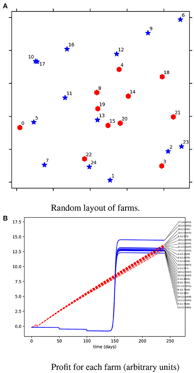
Figure 1. The profit generated (B) for a set of farms (A) randomly arranged on a 250 × 250 grid. Farms produce a crop that grows as a linear model (α = 0.028, β = 0.02), red hexagons, or as a logistic model (L = 5.8, k = 0.7, t0 = 150), blue stars. Red hexagon farms have an initial outlay of 0.25 and apply a treatment on day 10 with a cost of 0.35 and incur a daily uniform cost of 0.001 while blue star farms have an initial outlay of 0.15 and apply treatments on days 50 and 100 each with a cost of 0.25 and incur a daily uniform cost of 0.001. The positive interaction (on and between farms) is 0.3 and the negative interaction is -0.3 which decay with a spatial and temporal rate of γ = 0.07, ϕ = 0.008 respectively.
When farms produce different crops, the heterogeneity in the landscape drives differences in each farms profit. In Figure 1A we see that farm 10 and 17 produce a similar crop and are sufficiently close that they mutually benefit from each others treatment of their crops and so have the highest profit amongst the blue stars. Farm 13 has the lowest profit as they are surrounded by red hexagons, negatively impacting their crop while farms 16 and 22 are shielded from these negative impacts by farms 12 and 2 respectively. Similar shielding effects are observed by farm 14 and 20, which being closer to farms producing similar crops and simultaneously being shielded has the largest profit of all the red hexagons.
When we connect some farms, e.g., by a road or river, a mechanism for greater interaction with their neighbors exists. Modeling the effect of these connections (e.g., contaminants being unwittingly transported on vehicles, wildlife migrating between farms etc.) is complex and unique to each circumstance. In this toy model we make the simplification that connected farms are closer to each other so that the spatial decay of the interaction is decreased. In the results shown here we half the distance between connected farms. In Figure 2A we connect 0, 5, 13, 20, and 21 and observe the difference in their profit due to the increased interaction with distant more neighbors. We can see a decrease in profit for farm 20 due to the diminished shielding effects from farm 5, Figure 2B. Farm 21 benefits from the increase interaction with farm 20 while farm 0 is most affected due to lack of any shielding effects (suffering a decrease in profit after 240 days compared to farm 5 that only suffered a smalleer drop due to the increased interaction with farm 13).
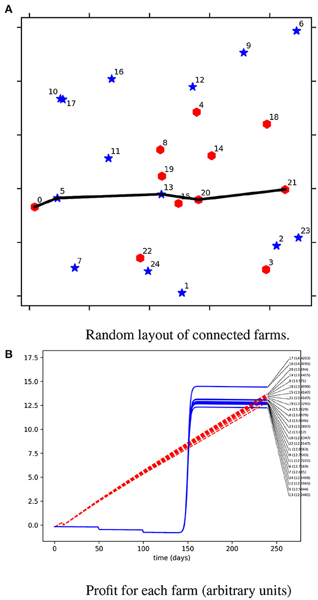
Figure 2. A similar random layout of farms as Figure 1 but where some farms are connected, e.g., by a road or river, that provides a mechanism for greater interaction with their neighbors. We model the interaction as a halving of the distance between connected farms. We can see that the shielding effects from neighboring farms is diminished leading to lower profit for farm 20, and that the presence of a connection decreases the profit for both farm 0 and 5 but the later's decrease is compensated by the neighboring similar farms. (A) Random layout of connected farms. (B) Profit for each farm (arbitrary units).
We can divide our landscape into a grid and calculate the level of contamination in the landscape at each point from every farmer's actions by calculating the distance from a farm and time an action was applied to the grid point. The contamination is calculated as the impact from each farm observed at each grid point using Equation (6). We plot this pollution for both types of farms in Figure 3 on day 240, the last day we calculate the profits in Figures 1B, 2B. The range of the interactions can be seen after 230 days for red hexagons and 140 days for blue stars. For earlier times, the effect will be stronger.
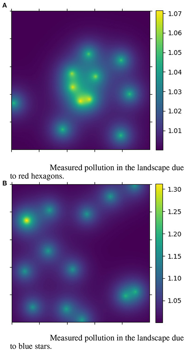
Figure 3. Measuring the effect of the actions on each farm after 240 days and the long lasting effects seen in the landscape. In each picture, the interactions between farms are positive and it is particularly clear in the case of red hexagons the beneficial effect of being close to neighbors that manage their farm in the same way. Actions were performed on day 10 in (A) and days 50 and 100 in (B).
We have introduced a toy model of food producing farms in a closed landscape that interact through the actions they perform on their farm. Despite the simplicity of the model a number of interesting and important results are obtained.
Firstly, the location of the farm within the network or landscape impacts on their ability to grow crops and produce a profit. We have seen that those on the edge of the network can receive less beneficial feedback than those in the interior. This is further compounded if they are neighbored by farms producing a different crop whose actions negatively impact the profit of the farm on the edge of the network. It is difficult to compare different network structures.
Secondly, there is an element of being shielded from the negative impacts of farms producing a different crop if you are surrounded by similar farms. This means that the optimal system of farms is a monoculture as it produces savings in fertilizer, pesticide, or other actions a farmer may use on their farm. In each of our networks, the monoculture gave better results than a mixed system though one particular farm in a circular network managed to have the same profit due to the shielding effects of its neighbors emphasing the importance of the location of a farm in the network. We have not included the effect on biodiversity in our simple model which would be impacted by a monoculture food production system.
Models like this make it easy to predict the level of pollutants (chemicals added on a farm that are measured outside the farm) in a landscape. In this simple model, we assume that impacts are relatively short ranged, and radially uniform but even with these simplifications we can see cooperative effects in the form of beneficial interactions with neighbors and shielding from detrimental effects. Modifications to any of these distributions are easy to implement for specific landscape conditions. Differences in the landscape terrain may influence wind patterns affecting the network of interactions between farms. Of course, the results of such a simple model may not be easily visible in reality where the interactions are more complicated and the landscape isn't smooth like we assume here.
Only very simple economic assumptions were made in creating this model and we do not consider this toy model to be an accurate representation of reality but it does show that at a broad level interactions between farms can affect the ability to grow food and modeling these interactions require specific focus and may not always be as simple as we have produced here. For example, cotton or apricot producers may obtain a mutual benefit from everyone using the same pesticide to control common pests (producing a positive interaction between farms) but also require a large amount of water and if not shared fairly can result in negative interactions, particularly in areas of water stress which is more complicated than the case considered here. Nevertheless, the competitive nature of these systems display similar patterns of mutual benefit and shielding.
The source code for the simulations can be found at: https://github.com/anthonyohare/ToyModelOfFoodProduction.
AO'H contrived and designed the model, performed the calculations and analysis, and wrote the manuscript.
The author declares that the research was conducted in the absence of any commercial or financial relationships that could be construed as a potential conflict of interest.
All claims expressed in this article are solely those of the authors and do not necessarily represent those of their affiliated organizations, or those of the publisher, the editors and the reviewers. Any product that may be evaluated in this article, or claim that may be made by its manufacturer, is not guaranteed or endorsed by the publisher.
The Supplementary Material for this article can be found online at: https://www.frontiersin.org/articles/10.3389/fams.2023.1058273/full#supplementary-material
1. Jones JW, Antle JM, Basso B, Boote KJ, Conant RT, Foster I, et al. Brief history of agricultural systems modeling. Agric Syst. (2017) 155:240–54. doi: 10.1016/j.agsy.2016.05.014
2. Reidsma P, Janssen S, Jansen J, van Ittersum MK. On the development and use of farm models for policy impact assessment in the European Union-a review. Agric Syst. (2018) 159:111–25. doi: 10.1016/j.agsy.2017.10.012
3. Porter J, Xie L, Challinor A, Cochrane K, Howden S, Iqbal M, et al. Chapter 7: food security and food production systems. In: Food security and food production systems. Climate Change 2014: Impacts, Adaptation, and Vulnerability. Part A: Global and Sectoral Aspects. Contribution of Working Group II to the Fifth Assessment Report of the Intergovernmental Panel on Climate Chan. Cambridge: Cambridge University Press (2014). p. 485–533. Available online at: https://eprints.whiterose.ac.uk/110945/
4. Nendel C, Zander P. Landscape Models to Support Sustainable Intensification of Agroecological Systems. Cambridge, UK: Burleigh Dodds Science Publishing Limited (2019). p. 321–54.
5. Rosenzweig C, Elliott J, Deryng D, Ruane AC, Müller C, Arneth A, et al. Assessing agricultural risks of climate change in the 21st century in a global gridded crop model intercomparison. Proc Natl Acad Sci USA. (2014) 111:3268–73. doi: 10.1073/pnas.1222463110
6. Keating B, Carberry PS, Hammer GL, Probert ME, Robertson MJ, Holzworth D, et al. An overview of APSIM, a model designed for farming systems simulation. Eur J Agron. (2003) 18: 267–88. doi: 10.1016/S1161-0301(02)00108-9
7. European Joint Programming Initiative for Agriculture Food Security Climate Change (FACCE JPI). Modelling Agriculture With Climate Change for Food Security–MACSUR (2022). Available online at: https://www.macsur.eu
8. Agricultural Model Intercomparison Improvement Project (AgMIP) community of experts. Agricultural Model Intercomparison and Improvement Project (2022). Available online at: https://agmip.org
9. University of Nebraska-Lincoln Wageningen University & Research. Global Yield Gap Atlas (2022). Available online at: https://www.yieldgap.org
10. Rindfuss RR, Entwisle B, Walsh SJ, An L, Badenoch N, Brown DG, et al. Land use change: complexity and comparisons. J Land Use Sci. (2008) 3:1–10. doi: 10.1080/17474230802047955
11. Parker DC, Manson SM, Janssen MA, Hoffmann MJ, Hoffmann MJ, Deadman P. Multi-agent systems for the simulation of land-use and land-cover change: a review. Ann Assoc Am Geograph. (2003) 92:314–37. doi: 10.1111/1467-8306.9302004
12. Noszczyk T. A review of approaches to land use changes modeling. Hum Ecol Risk Assess. (2019) 25:1377–405. doi: 10.1080/10807039.2018.1468994
13. Houghton RA, House JI, Pongratz J, van der Werf GR, DeFries RS, Hansen MC, et al. Carbon emissions from land use and land-cover change. Biogeosciences. (2012) 9:5125–42. doi: 10.5194/bg-9-5125-2012
14. Nguyen TTH, Doreau M, Eugène M, Corson MS, Garcia-Launay F, Chesneau G, et al. Effect of farming practices for greenhouse gas mitigation and subsequent alternative land use on environmental impacts of beef cattle production systems. Animal. (2013) 7:860–9. doi: 10.1017/S1751731112002200
15. Nelson GC, Valin H, Sands RD, Havlik P, Ahammad H, Deryng D, et al. Climate change effects on agriculture: economic responses to biophysical shocks. Proc Natl Acad Sci USA. (2014) 111:3274–9. doi: 10.1073/pnas.1222465110
16. Patz JA, Norris DE. Land use change and human health. In:DeFries RS, Asner GP, Houghton RA, , editors. Geophysical Monograph Series. vol. 153. Washington, D C: American Geophysical Union (2004). p. 159–67.
17. Jacques P, Jacques JR. Monocropping cultures into ruin: the loss of food varieties and cultural diversity. Sustainability. (2012) 4:2970–97. doi: 10.3390/su4112970
18. Crist E, Mora C, Engelman R. The interaction of human population, food production, and biodiversity protection. Science. (2017) 356:260–4. doi: 10.1126/science.aal2011
19. Guillem EE, Murray-Rust D, Robinson DT, Barnes A, Rounsevell M. Modelling farmer decision-making to anticipate tradeoffs between provisioning ecosystem services and biodiversity. Agric Syst. (2015) 137:12–23. doi: 10.1016/j.agsy.2015.03.006
20. Antle JM, Basso B, Conant RT, Godfray HCJ, Jones JW, Herrero M, et al. Towards a new generation of agricultural system data, models and knowledge products: design and improvement. Agric Syst. (2017) 155:255–68. doi: 10.1016/j.agsy.2016.10.002
21. Viana CM, Freire D, Abrantes P, Rocha J, Pereira P. Agricultural land systems importance for supporting food security and sustainable development goals: a systematic review. Sci Total Environ. (2022) 806:150718. doi: 10.1016/j.scitotenv.2021.150718
22. Parker DC, Meretsky VJ. Measuring pattern outcomes in an agent-based model of edge-effect externalities using spatial metrics. Agric Ecosyst Environ. (2004) 101:233–50. doi: 10.1016/j.agee.2003.09.007
23. Prskawetz A, Feichtinger G, Luptacik M, Milik A, Wirl F, Hof F, et al. Endogenous growth of population and income depending on resource and knowledge. Eur J Populat. (1998) 14:305–31. doi: 10.1007/BF02863319
24. Verma BK, Pushpavanam S. Population interaction based on occupation: agriculturists and industrialists. In: 2016 AIChE Annual Meeting. (2016). Available online at: https://aiche.confex.com/aiche/2016/webprogram/Paper463759.html
25. Tamura R. Human capital and the switch from agriculture to industry. J Econ Dyn Control. (2002) 27:207–42. doi: 10.1016/S0165-1889(01)00032-X
26. Matthews R, Gilbert N, Roach A, Polhill JG, Gotts NM. Agent-based land-use models: a review of applications. Landscape Ecol. (2007) 22:1447–59. doi: 10.1007/s10980-007-9135-1
27. Rounsevell MDA, Arneth A, Alexander P, Brown DG, de Noblet-Ducoudré N, Ellis E, et al. Towards decision-based global land use models for improved understanding of the Earth system. Earth Syst Dyn. (2014) 5:117–37. doi: 10.5194/esd-5-117-2014
28. Groeneveld J, Mller B, Buchmann CM, Dressler G, Guo C, Hase N, et al. Theoretical foundations of human decision-making in agent-based land use models a review. Environ Model Software. (2017) 87:39–48. doi: 10.1016/j.envsoft.2016.10.008
29. Ren Y, Lü Y, Comber A, Fu B, Harris P, Wu L. Spatially explicit simulation of land use/land cover changes: current coverage and future prospects. Earth Sci Rev. (2019) 190:398–415. doi: 10.1016/j.earscirev.2019.01.001
30. An L. Modelling human decisions in coupled human and natural systems: review of agent-based models. Ecol Model. (2012) 220:25–36. doi: 10.1016/j.ecolmodel.2011.07.010
31. Kelley H, Evans TP, Evans TP, Evans T. The relative influences of land-owner and landscape heterogeneity in an agent-based model of land-use. Ecol Econ. (2011) 70:1075–87. doi: 10.1016/j.ecolecon.2010.12.009
32. Smajgl A, Brown DG, Valbuena D, Huigen M. Empirical characterisation of agent behaviours in socio-ecological systems. Environ Model Software. (2011) 26: 837–44. doi: 10.1016/j.envsoft.2011.02.011
33. Filatova T, Verburg PH, Parker DC, Stannard CA. Spatial agent-based models for socio-ecological systems: challenges and prospects. Environ ModelSoftware. (2013) 45:1–7. doi: 10.1016/j.envsoft.2013.03.017
34. Nolan J, Parker DC, van Kooten GC, van Kooten GC, Berger T. An overview of computational modelling in agricultural and resource economics. Can J Agric Econ. (2009) 57:417–29. doi: 10.1111/j.1744-7976.2009.01163.x
Keywords: competition, cooperation, agent-based modeling, agricultural system model, food production model
Citation: O'Hare A (2023) A toy model of food production in a connected landscape. Front. Appl. Math. Stat. 9:1058273. doi: 10.3389/fams.2023.1058273
Received: 30 September 2022; Accepted: 16 January 2023;
Published: 02 February 2023.
Edited by:
Raluca Eftimie, University of Franche-Comté, FranceReviewed by:
Babita K. Verma, Johns Hopkins University, United StatesCopyright © 2023 O'Hare. This is an open-access article distributed under the terms of the Creative Commons Attribution License (CC BY). The use, distribution or reproduction in other forums is permitted, provided the original author(s) and the copyright owner(s) are credited and that the original publication in this journal is cited, in accordance with accepted academic practice. No use, distribution or reproduction is permitted which does not comply with these terms.
*Correspondence: Anthony O'Hare,  YW50aG9ueS5vaGFyZUBzdGlyLmFjLnVr
Disclaimer: All claims expressed in this article are solely those of the authors and do not necessarily represent those of their affiliated organizations, or those of the publisher, the editors and the reviewers. Any product that may be evaluated in this article or claim that may be made by its manufacturer is not guaranteed or endorsed by the publisher.
Research integrity at Frontiers
Learn more about the work of our research integrity team to safeguard the quality of each article we publish.