Vaccination and variants: A COVID-19 multi-strain model evolution for the Philippines

Coronavirus disease 2019 (COVID-19) management and response is a challenging task due to the uncertainty and complexity of the nature surrounding the virus. In particular, the emergence of new variants and the polarizing response from the populace complicate government efforts to control the pandemic. In this study, we developed a compartmental model that includes (1) a vaccinated compartment, (2) reinfection after a particular time, and (3) COVID-19 variants dominant in the Philippines. Furthermore, we incorporated stochastic terms to capture uncertainty brought about by the further evolution of the new variants and changing control measures via parametric perturbation. Results show the importance of booster shots that increase the vaccine-induced immunity duration. Without booster shots, simulations showed that the dominant strain would still cause significant infection until 31 December 2023. Moreover, our stochastic model output showed significant variability in this case, implying greater uncertainty with future predictions. All these adverse effects, fortunately, can be effectively countered by increasing the vaccine-induced immunity duration that can be done through booster shots.

1. Introduction

Since the emergence of coronavirus disease 2019 (COVID-19) in Wuhan, its causative agent, severe acute respiratory syndrome coronavirus 2 (SARS-CoV-2), has been rapidly evolving into new variants [1]. This emergence is expected as, like any virus, SARS-CoV-2 continues to mutate from time to time. So far, the World Health Organization (WHO) has identified five variants of concern, namely, Alpha, Beta, Gamma, Delta, and Omicron. These are the variants considered the most transmissible and dominant that are circulating the world [2]. While vaccine has been available, the campaign has suffered a series of setbacks and there are many issues leading to vaccine hesitancy [3, 4]. In the Philippines, the slow vaccine rollout, limited testing capacity, weak genomics surveillance, a fragile healthcare system, and a large informal economy contributed more to the many issues related to COVID-19. The latter is a social cost as few people can afford not to work but are forced to stay home in overcrowded housing. These factors exacerbated the situation as they gave the virus a perfect environment to mutate, feeding through a continuous supply of susceptibles.

Hence, a question of much importance is how to reduce COVID-19 transmission. In doing so, an approach of balancing the efforts on the vaccination campaign (booster shots amidst reinfection because of mutating variants and waning immunity), and preparedness of the healthcare system coupled with public health and social measures is a must. While the government is trying to strike a balance, the race between vaccination and fast mutating variants remains the biggest challenge.

Many computational modeling studies have investigated COVID-19 dynamics in the Philippines. For instance, in Arcede et al. [5], an SEIR-type model is constructed whose infected can either be symptomatic or not. The result shows that treating symptomatic alone does not reduce the spread. However, managing the number of susceptible does, which containment and vaccines have a significant impact role to play. Later, the same model was used to investigate the implemented non-pharmaceutical interventions (NPI) in the country [6]. Here, NPIs include lockdown, social distancing, mass testing, and strengthening the healthcare system. The study provided a choice for the government to implement the control by indicating economic cost (low, high) given no vaccine availability. In Bock et al. [7], an agent-based SIR model was used to investigate the prevalence of COVID-19 in two neighboring cities in Northern Mindanao, particularly in Iligan and Cagayan de Oro. The result shows that social distancing and age-specific quarantine can effectively slow down contagion. Furthermore, social distancing combined with an effective testing strategy can keep the epidemic at bay and prevent it from becoming a critical epidemic. In Arcede et al. [8], a regional COVID-19 model has been constructed in the cities mentioned earlier and in the Northern Mindanao region as a whole. The model is tailored to fit early transmission; hence appropriate models are suggested when laboratory-based disease reports are available. In [9], Mammeri et al. extended their SEIR-type model to account the spatial movement of individuals. Given five main islands and five main airports in the Philippines as nodes with index case assumed to start from Manila airport on day 1, their simulation show remarkably close similarity to what happened in the Philippines during its first 140 days. Studies mentioned do not deal with vaccination control. However, recent articles deal with vaccination strategies in the Philippine context. For instance, in [10], optimal control was used to investigate existing policy interventions, including vaccination rollouts, community quarantines, and simulated virus outbreaks. They found that early and effective implementation of precautionary measures such as community quarantines are crucial for containing outbreaks. They also found that even if vaccinations do not suffice, expanding the vaccine supply reduces the need for more resource-intensive interventions. Moreover, in Caga-anan et al. [11], a model with a delay on the vaccination compartment was constructed to study the impact of vaccination efforts on disease progression and herd immunity. The result shows that timely vaccination is preferred to maximize impact. They also assessed the performance of different vaccine brands in the model, showing Pfizer-BioNTech with the best results. Finally, some models were proposed for allocating resources. For instance, optimizing the location of vaccination sites implemented in San Juan Philippines [12] and distribution of COVID-19 testing kits in DOH-accredited testing centers in the country [13]. All studies mentioned earlier do not account explicitly for COVID-19 variants and randomness.

In this study, we evaluate the impact of vaccination and its waning induced immunity, as well as the uncertainties related to future mitigation policies and the further evolution of the virus, given the three variants that are circulating dominantly in the country.

2. Model formulation

2.1. Deterministic model

In this study, we divided the population into eight compartments, namely, susceptible (S), vaccinated (V), infected by the original strain (I₁), infected by the Delta variant (I₂), infected by the Omicron variant (I₃), confirmed (C), recovered (R), and dead (D). Figure 1 shows the dynamics of the model. The model considers the following facts. First, vaccines do not provide lasting immunity. Hence, vaccinated people will be back to being susceptible after some time. Second, reported confirmed cases do not show the full extent of the infection. Third, estimates of unreported cases are not being accounted for. Finally, recovered individuals (from natural infection) also do not have lasting immunity against the virus; hence, both vaccinated and recovered individuals may return to the susceptible population after some time. In the model, we assume density-dependent transmission rates.

FIGURE 1

Figure 1. Model dynamics of COVID-19 with three strains.

An infected individual by any of the variants can infect people in compartment S. We assume that vaccinated people in V are immune to any of the variants. The parameter β_i denotes the transmission rate of the disease caused by the ith strain. The parameter α represents the level of control measures implemented to limit the transmission. The parameter ν denotes the vaccination rate of susceptible people. The parameters λ₁ and λ₂ denote the vaccine immunity waning rate and natural immunity waning rate, respectively. The parameter ϵ denotes the proportion of infections detected and confirmed through testing also known as detection rate. We also have the removal rate from C given by δ. Finally, the recovery rate from unconfirmed infections caused by the ith strain is denoted as γ_i and the probability to recover from the infection is denoted as ρ. The parameters are summarized in Table 1.

TABLE 1

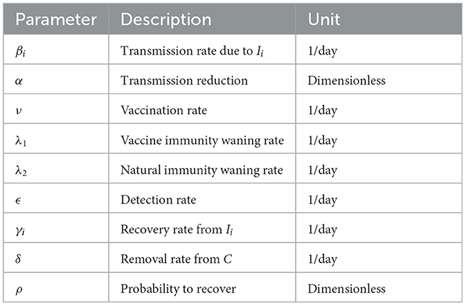
Table 1. Parameters of the model.

In this study, we adapted a closed population model, i.e., we did not consider natural birth and death rates. We denote by N₀ the total number of population at the start. The dynamics of our model is governed by the following system of ordinary differential equations (ODE):

$\begin{array}{ll}\frac{dS}{dt}=-\alpha ({\beta }_1{I}_1+{\beta }_2{I}_2+{\beta }_3{I}_3)\frac{S}{N_0}-\nu S+{\lambda }_{1}V+{\lambda }_{2}R& (1)\end{array}$

$\begin{array}{ll}\frac{dV}{dt}=\nu S-{\lambda }_{1}V& (2)\end{array}$

$\begin{array}{ll}\frac{d{I}_1}{dt}=\alpha {\beta }_1{I}_1\frac{S}{N_0}-({\gamma }_1+ϵ)I_1& (3)\end{array}$

$\begin{array}{ll}\frac{d{I}_2}{dt}=\alpha {\beta }_2{I}_2\frac{S}{N_0}-({\gamma }_2+ϵ)I_2& (4)\end{array}$

$\begin{array}{ll}\frac{d{I}_3}{dt}=\alpha {\beta }_3{I}_3\frac{S}{N_0}-({\gamma }_3+ϵ)I_3& (5)\end{array}$

$\begin{array}{ll}\frac{dC}{dt}=ϵI_1+ϵI_2+ϵI_3-\delta C& (6)\end{array}$

$\begin{array}{ll}\frac{dR}{dt}={\gamma }_1{I}_1+{\gamma }_2{I}_2+{\gamma }_3{I}_3+\delta \rho C-{\lambda }_{2}R& (7)\end{array}$

$\begin{array}{ll}\frac{dD}{dt}=\delta (1-\rho )C.& (8)\end{array}$

2.2. Stochastic model

As will be seen in Section 5, the third strain will become dominant as time goes on. We acknowledge that we need to accommodate future uncertainties in our simulation. Hence, we modify our ODE model to add stochasticity. We apply parametric perturbation to the reduced transmission rate αβ₃. The resulting system with stochastic differential equations (SDE) is as follows:

$\begin{array}{l}dS=\left[-\alpha ({\beta }_1{I}_1+{\beta }_2{I}_2+{\beta }_3{I}_3)\frac{S}{N_0}-\nu S+{\lambda }_{1}V+{\lambda }_{2}R\right]dt\\ -\sigma I_3\frac{S}{N_0}dB\\ dV=\left[\nu S-{\lambda }_{1}V\right]dt\\ d{I}_1=\left[\alpha {\beta }_1{I}_1\frac{S}{N_0}-({\gamma }_1+ϵ)I_1\right]dt\end{array}$

$\begin{array}{ll}d{I}_2=\left[\alpha {\beta }_2{I}_2\frac{S}{N_0}-({\gamma }_2+ϵ)I_2\right]dt& (9)\end{array}$

$\begin{array}{l}d{I}_3=\left[\alpha {\beta }_3{I}_3\frac{S}{N_0}-({\gamma }_3+ϵ)I_3\right]dt+\sigma I_3\frac{S}{N_0}dB\\ dC=\left[ϵI_1+ϵI_2+ϵI_3-\delta C\right]dt\\ dR=\left[{\gamma }_1{I}_1+{\gamma }_2{I}_2+{\gamma }_3{I}_3+\delta \rho C-{\lambda }_{2}R\right]dt\\ dD=\left[\delta (1-\rho )C\right]dt,\end{array}$

where dB/dt is the white noise, i.e., the derivative of the standard Brownian motion B(t), and σ > 0 denotes the intensity of that noise.

3. Qualitative analysis of the ODE model

Since we have a close system and N₀ = S + V + I₁ + I₂ + I₃ + C + R + D, we may just consider the system (1)–(7), i.e., without D. To find the disease-free equilibrium (DFE) (a steady-state solution of an epidemic model with all infected variables equals to zero), we equate Equations (1)–(7) to zero and the infective compartments I₁, I₂, I₃, and C equal to 0. We obtain a solution, which is the DFE given by (S^*, V^*, 0, 0, 0, 0, 0), where $S^{*}=\frac{{\lambda }_1{V}^{*}}{\nu }$.

3.1. Reproduction number

By definition, the basic reproduction number ${{R}}_0$ denotes the average number of individuals directly infected by a single infected individual over the duration of its infectious period in a population without any deliberate intervention to stop its spread. We will compute ${{R}}_0$ using the next generation matrix method defined by Diekman et al. [14] and van den Driessche and Watmough [15]. Let X be the vector of the infected classes and Y be the vector of the other classes. Let ${F}(X,Y)$ be the vector of new infection rates (flows from Y to X) and let ${V}(X,Y)$ be the vector of all other rates (not new infections). Then, we have

$\begin{array}{l}{F}=\left[\begin{array}{c}\alpha {\beta }_1{I}_1\frac{S}{N_0}\\ \alpha {\beta }_2{I}_2\frac{S}{N_0}\\ \alpha {\beta }_3{I}_3\frac{S}{N_0}\\ ϵI_1+ϵI_2+ϵI_3\end{array}\right],{V}=\left[\begin{array}{c}({\gamma }_1+ϵ)I_1\\ ({\gamma }_2+ϵ)I_2\\ ({\gamma }_3+ϵ)I_3\\ \delta C\end{array}\right].\end{array}$

Evaluating the derivatives of ${F}$ and ${V}$ at the DFE, we are led to the following matrices

$F=\left[\begin{array}{cccc}\alpha {\beta }_1\frac{S^{*}}{N_0}& 0& 0& 0\\ 0& \alpha {\beta }_2\frac{S^{*}}{N_0}& 0& 0\\ 0& 0& \alpha {\beta }_3\frac{S^{*}}{N_0}& 0\\ ϵ& ϵ& ϵ& 0\end{array}\right],V=\left[\begin{array}{cccc}{\gamma }_1+ϵ& 0& 0& 0\\ 0& {\gamma }_2+ϵ& 0& 0\\ 0& 0& {\gamma }_3+ϵ& 0\\ 0& 0& 0& \delta \end{array}\right].$

Hence, the next generation matrix is given by

$\begin{array}{l}K=F{V}^{-1}=\left[\begin{array}{cccc}\left(\frac{\alpha {\beta }_1}{{\gamma }_1+ϵ}\right)\frac{S^{*}}{N_0}& 0& 0& 0\\ 0& \left(\frac{\alpha {\beta }_2}{{\gamma }_2+ϵ}\right)\frac{S^{*}}{N_0}& 0& 0\\ 0& 0& \left(\frac{\alpha {\beta }_3}{{\gamma }_3+ϵ}\right)\frac{S^{*}}{N_0}& 0\\ \frac{ϵ}{{\gamma }_1+ϵ}& \frac{ϵ}{{\gamma }_2+ϵ}& \frac{ϵ}{{\gamma }_3+ϵ}& 0\end{array}\right].\end{array}$

The eigenvalues of K are the following: ${\eta }_1=\left(\frac{\alpha {\beta }_1}{{\gamma }_1+ϵ}\right)\frac{S^{*}}{N_0}$, ${\eta }_2=\left(\frac{\alpha {\beta }_2}{{\gamma }_2+ϵ}\right)\frac{S^{*}}{N_0}$, ${\eta }_3=\left(\frac{\alpha {\beta }_3}{{\gamma }_3+ϵ}\right)\frac{S^{*}}{N_0}$, and η₄ = 0. The eigenvalue η₁ is associated with strain 1 and gives rise to the basic reproduction number ${{R}}_1=\left(\frac{{\lambda }_1\alpha {\beta }_1}{\nu \left({\gamma }_1+ϵ\right)}\right)\frac{V^{*}}{N_0}$. Similarly, eigenvalue η₂ associated with strain 2 corresponds to the basic reproduction number ${{R}}_2=\left(\frac{{\lambda }_1\alpha {\beta }_2}{\nu \left({\gamma }_2+ϵ\right)}\right)\frac{V^{*}}{N_0}$, and eigenvalue η₃ associated with strain 3 corresponds to ${{R}}_3=\left(\frac{{\lambda }_1\alpha {\beta }_3}{\nu \left({\gamma }_3+ϵ\right)}\right)\frac{V^{*}}{N_0}$. Finally, we take ${{R}}_0=max\left\{{{R}}_1,{{R}}_2,{{R}}_3\right\}.$

3.2. Stability analysis of the DFE

Theorem 3.1. The disease-free equilibrium $x_0=\left(S^{*},V^{*},0,0,0,0,0,D^{*}\right)$, where $S^{*}=\frac{{\lambda }_1{V}^{*}}{\nu }$ and $D^{*}=N_0-\left(S^{*}+V^{*}\right)$ of system (1)-(8) is globally asymptotically stable.

Proof. Consider that

$\begin{array}{ll}D\left(t\right)-D\left(0\right)={\displaystyle {\int }_0^t}\delta \left(1-\rho \right)C\left(s\right)ds& \left(10\right)\end{array}$

and

$\begin{array}{ll}{D}^{*}-D\left(0\right)={\displaystyle {\int }_0^{+\infty }}\delta \left(1-\rho \right)C\left(s\right)ds.& \left(11\right)\end{array}$

This is finite, since D is bounded. Hence, δ(1 − ρ)C(t) → 0 as t → +∞. Since δ(1 − ρ) > 0, we have C(t) → 0 as t → +∞. Using the same argument and noting that

$\begin{array}{ll}{C}^{*}-C\left(0\right)={\displaystyle {\int }_0^{+\infty }}ϵI_1\left(s\right)+ϵI_2\left(s\right)+ϵI_3\left(s\right)-\delta C\left(s\right)ds,& \left(12\right)\end{array}$

we also have I₁(t), I₂(t), I₃(t) → 0 as t → +∞. Similar deduction can be used to show that R(t) → 0 as t → +∞, using Equation (7). □

We may define the effective reproduction number associated with strain i by

$\begin{array}{ll}{{R}}_i^e\left(t\right)=\left(\frac{{\lambda }_1\alpha {\beta }_i}{\nu ({\gamma }_i+ϵ)}\right)\frac{V\left(t\right)}{N_0}.& \left(13\right)\end{array}$

Compared to the basic reproduction number ${{R}}_0$, the effective reproduction number ${{R}}_i^e\left(t\right)$ denotes the average number of new infections associated with strain i, at time t, caused by a single infected individual, considering that in the population at this time, there are already some individuals who are no longer susceptible.

4. Existence of solution for the SDE Model

Let $\left(\Omega ,{F},{\left\{{{F}}_t\right\}}_{t\ge 0},\mathbb{P}\right)$ be a complete probability space with filtration ${\left\{{{F}}_t\right\}}_{t\ge 0}$ satisfying the usual conditions (i.e., it is increasing and right continuous while ${{F}}_0$ contains all ℙ-null sets). Let ${ℝ}_{+}^8=\left\{x_i>0:i=1,2,...,8\right\}$. Let B(t) be a Brownian motion defined on the complete probability space Ω. Then, we have the following theorem showing that the stochastic system (9) has a unique non-negative global solution.

Theorem 4.1. For any given initial value $x_0\in {ℝ}_{+}^8$, there is a unique solution x(t) of system (9) on t ≥ 0, and the solution will remain in ${ℝ}_{+}^8$ with probability 1, namely, $x\left(t\right)\in {ℝ}_{+}^8$ for all t ≥ 0 almost surely.

Proof. Since the coefficients of system (9) satisfy the local Lipschitz condition, it implies that for any given initial value $x_0\in {ℝ}_{+}^8$, there is a unique local solution x(t) for every t ∈ [0, τ_e), where τ_e is the explosion time. To prove that the solution is global, we need to show that τ_e = ∞. To do so, we let s₀ ≥ 1 be sufficiently large so that all components of x₀ are contained in the interval [1/s₀, s₀]. For each integer s ≥ s₀, we define the stopping time by

${\tau }_s=inf\left\{t\in \left[0,{\tau }_e\right):\text{at least one of }S,V,I_1,I_2,I_3,C,R,\text{or}D\in \left(1/s,s\right)\right\}.$

Clearly, τ_s is increasing as s → ∞. Let ${\tau }_{\infty }=\underset{s\to \infty }{lim}{\tau }_s$, then τ_e ≥ τ_∞ almost surely. If we can show that τ_∞ = ∞ a.s., then τ_e = ∞ and $x\left(t\right)\in {ℝ}_{+}^8$ a.s. for all t ≥ 0.

Suppose τ_∞ < ∞, then there exists T > 0 such that ℙ{τ_∞ ≤ T} > ϵ for all ϵ ∈ (0, 1). Hence, there is an integer s₁ ≥ s₀ such that

$\begin{array}{ll}\mathbb{P}\left\{{\tau }_s\le T\right\}>ϵ,\text{for every }s\ge s_1.& \left(14\right)\end{array}$

Let a ${{C}}^2-$ function $U:{ℝ}_{+}^8\to {ℝ}_{+}^8$ be defined by

$\begin{array}{l}U\left(x\right)=S-1-ln\left(S\right)+V-1-ln\left(V\right)+I_1-1-ln\left(I_1\right)\\ +I_2-1-ln\left(I_2\right)\\ +I_3-1-ln\left(I_3\right)+C-1-ln\left(C\right)+R-1-ln\left(R\right)\\ +D-1-ln\left(D\right).& \left(15\right)\end{array}$

Using Itô formula on Equation (15), we have

$dU=LUdt+\sigma \frac{I_3}{N_0}dB-\sigma \frac{S}{N_0}dB,$

where

$\begin{array}{l}LU=\left(1-\frac{1}{S}\right)\left[-\alpha \left({\beta }_1{I}_1+{\beta }_2{I}_2+{\beta }_3{I}_3\right)\frac{S}{N_0}-\nu S+{\lambda }_{1}V+{\lambda }_{2}R\right]\\ +\frac{1}{2}{\sigma }^2\frac{I_3^2}{N_0^2}+\left(1-\frac{1}{V}\right)\left[\nu S-{\lambda }_{1}V\right]+\left(1-\frac{1}{I_1}\right)\\ \left[\alpha {\beta }_1{I}_1\frac{S}{N_0}-\left({\gamma }_1+ϵ\right)I_1\right]+\left(1-\frac{1}{I_2}\right)\\ \left[\alpha {\beta }_2{I}_2\frac{S}{N_0}-\left({\gamma }_2+ϵ\right)I_2\right]+\left(1-\frac{1}{I_3}\right)\\ \left[\alpha {\beta }_3{I}_3\frac{S}{N_0}-\left({\gamma }_3+ϵ\right)I_3\right]+\frac{1}{2}{\sigma }^2\frac{S^2}{N_0^2}+\left(1-\frac{1}{C}\right)\\ \left[ϵ\left(I_1+I_2+I_3\right)-\delta C\right]+\left(1-\frac{1}{R}\right)\\ \left[{\gamma }_1{I}_1+{\gamma }_2{I}_2+{\gamma }_3{I}_3+\delta \rho C-{\lambda }_{2}R\right]\\ +\left(1-\frac{1}{D}\right)\left[\delta \left(1-\rho \right)C\right]\le \nu +{\lambda }_1+\left({\gamma }_1+{\gamma }_2+{\gamma }_3\right)+3ϵ\\ +\delta +{\lambda }_2+\frac{1}{2}{\sigma }^2\frac{I_3^2}{N_0^2}+\frac{1}{2}{\sigma }^2\frac{S^2}{N_0^2}+\alpha {\beta }_1\frac{I_1}{N_0}+\alpha {\beta }_2\frac{I_2}{N_0}\\ +\alpha {\beta }_3\frac{I_3}{N_0}\le \nu +{\lambda }_1+\left({\gamma }_1+{\gamma }_2+{\gamma }_3\right)+3ϵ+\delta +{\lambda }_2\\ +{\sigma }^2\frac{N_0^2}{N_0^2}+\left[\alpha {\beta }_1+\alpha {\beta }_2+\alpha {\beta }_3\right]\frac{N_0}{N_0}\le \nu +{\lambda }_1\\ +\left({\gamma }_1+{\gamma }_2+{\gamma }_3\right)+3ϵ+\delta +{\lambda }_2+{\sigma }^2+\alpha {\beta }_1+\alpha {\beta }_2+\alpha {\beta }_3\\ :=K.\end{array}$

Note that K is a positive constant independent of the variables S, V, I₁,I₂, I₃, C, R, and D, and time t.

Thus,

$\begin{array}{ll}dU=Kdt+\sigma \frac{I_3}{N_0}dB-\sigma \frac{S}{N_0}dB.& \left(16\right)\end{array}$

Therefore, if t₁ ≤ T,

$\begin{array}{lll}{\displaystyle {\int }_0^{{\tau }_s\wedge t_1}}dU& \le {\displaystyle {\int }_0^{{\tau }_s\wedge t_1}}Kdt+{\displaystyle {\int }_0^{{\tau }_s\wedge t_1}}\frac{\sigma }{N_0}\left(I_3-S\right)dB\left(t\right),& \left(17\right)\end{array}$

where τ_s ∧ t₁ = min{τ_s, t₁}. Taking expectations to both sides of (17), we obtain

$\begin{array}{lll}𝔼\left[{\displaystyle {\int }_0^{{\tau }_s\wedge t_1}}dU\right]& \le 𝔼\left[{\displaystyle {\int }_0^{{\tau }_s\wedge t_1}}Kdt\right]+𝔼\left[{\displaystyle {\int }_0^{{\tau }_s\wedge t_1}}\frac{\sigma }{N_0}\left(I_3-S\right)dB\left(t\right)\right].& \left(18\right)\end{array}$

By properties of Itô integral, we have

$\begin{array}{ll}𝔼U\left(F\left({\tau }_s\wedge t_1\right),C\left({\tau }_s\wedge t_1\right),\rho \left({\tau }_s\wedge t_1\right)\right)\le U\left(F\left(0\right),C\left(0\right),\rho \left(0\right)\right)& \left(19\right)\end{array}$

$\begin{array}{l}+𝔼\left[{\displaystyle {\int }_0^{{\tau }_s\wedge t_1}}Kdt\right]\\ \le U_0+KT<\infty ,\end{array}$

where U₀ = U(x₀). By Gronwall's inequality,

$\begin{array}{ll}𝔼V\left(F\left({\tau }_s\wedge t_1\right),C\left({\tau }_s\wedge t_1\right),\rho \left({\tau }_s\wedge t_1\right)\right)\le U_0{e}^{KT}<\infty .& \left(20\right)\end{array}$

Let Ω_s = {τ_s ≤ T} for any s ≥ s₁. Then, by (14), we have ℙ(Ω_s) ≥ ϵ. Note that for every ω ∈ Ω_s, there is at least one of S(τ_s, ω), V(τ_s, ω), I₁(τ_s, ω), I₂(τ_s, ω), I₃(τ_s, ω), C(τ_s, ω), R(τ_s, ω), and D(τ_s, ω) that is equal to either s or 1/s. Consequently, U(x(τ_s, ω)) is no less than either

$s-1-ln\left(s\right)\text{or }\frac{1}{s}-1-ln\left(\frac{1}{s}\right)=\frac{1}{s}-1+ln\left(s\right).$

Thus,

$U\left(x\left({\tau }_s,\omega \right)\right)\ge \left[s-1-ln\left(s\right)\right]\wedge \left[\frac{1}{s}-1+ln\left(s\right)\right].$

It then follows from Equation (14) and Equation (21) that

$\begin{array}{l}{U}_0{e}^{KT}\ge 𝔼\left[1_{{\Omega }_s}\left(\omega \right)U\left(x\left({\tau }_s,\omega \right)\right)\right]\\ \ge ϵ\left[s-1-ln\left(s\right)\wedge \frac{1}{s}-1+ln\left(s\right)\right],\end{array}$

where 1_Ωs is an indicator function of Ω_s. Letting s → ∞, then we have

$\infty >U_0{e}^{KT}\ge \infty ,$

which yields the contradiction. Therefore, we must have τ_∞ = ∞, almost surely.□

5. Numerical simulations

Data on confirmed cases used in parameter calibration are from the COVID-19 Data Repository by the Center for Systems Science and Engineering (CSSE) at Johns Hopkins University (JHU) [16]. The data are publicly available and so ethical approval is not required. The data are from 1 January 2021 (Day 0) to 28 June 2022 (Day 543). Values of some parameters and initial conditions are taken or estimated from sources as indicated in Tables 2, 3. We note that the parameter α varies over time as controls implemented by the government also vary. Hence, we considered α as a piecewise constant function, as shown in Table 2, where the dates correspond to the noticeable changes in the control measures implemented by the government.

TABLE 2

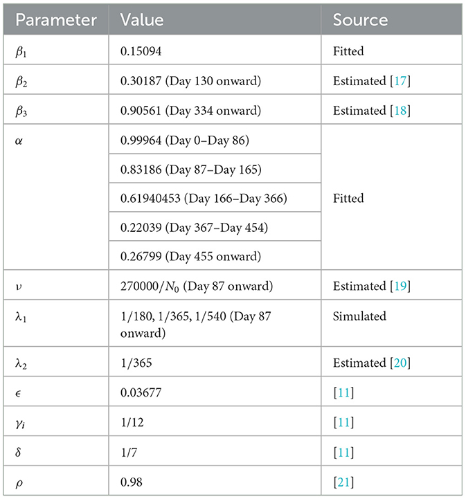
Table 2. Values of the parameters used in the simulations.

TABLE 3

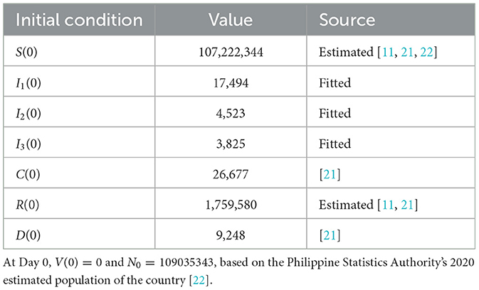
Table 3. Initial conditions used in the simulations.

To obtain the fitted values for the parameters β₁ and α, and the initial conditions I₁(0), I₂(0), and I₃(0), we minimized a non-linear least square function given by the sum of the square of the difference of the data and the model output. The optimization problem is solved using the approximate Bayesian computation approach combined with the Levenberg–Marquardt algorithm [23–25]. Visualization of the optimization result is given in Figure 2. In Figure 3, we plotted the evolution of the three variants based on the optimization result.

FIGURE 2

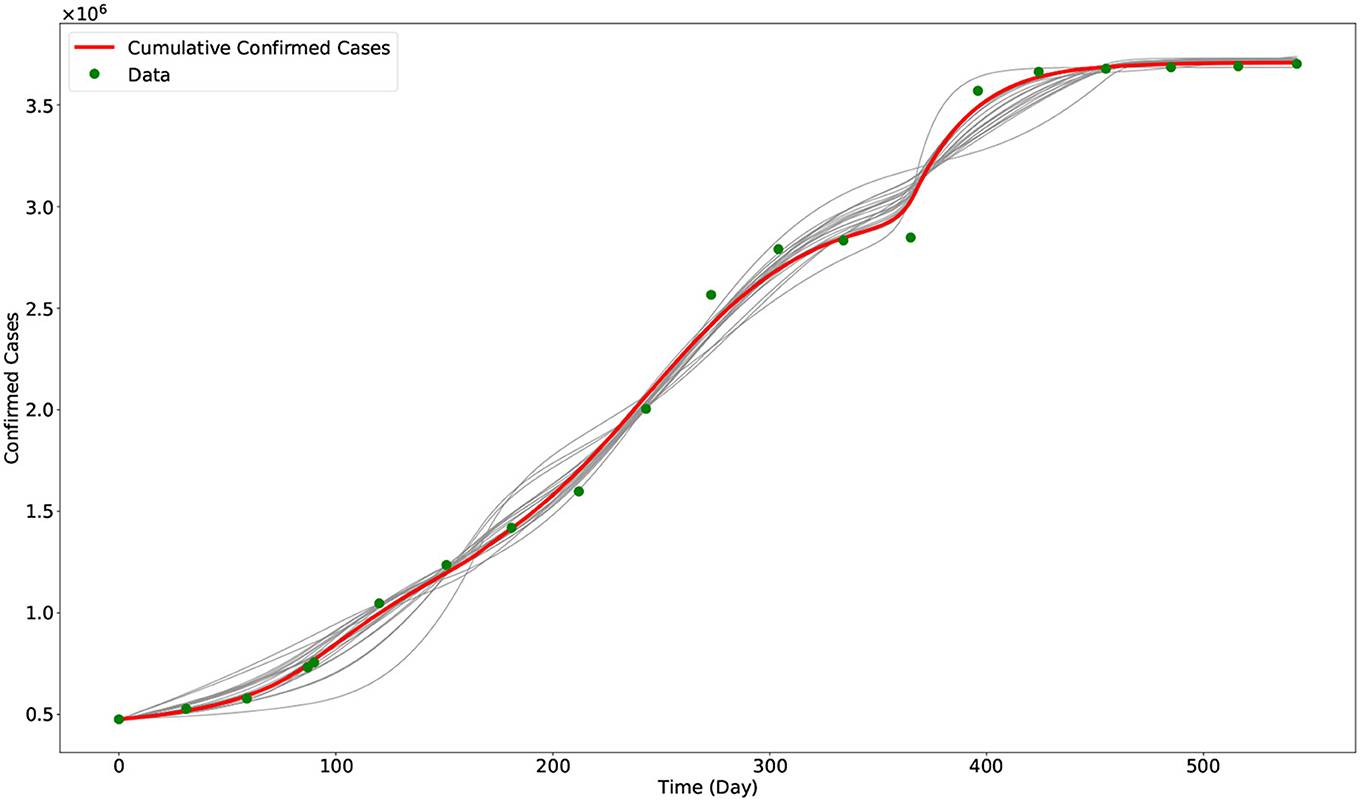
Figure 2. Output of the model with calibrated parameters compared with data. The gray curves represent the other outputs of the approximate Bayesian computation approach, while the red curve represents the best fit model output (i.e., using the parameters in Table 2). The green dots are the data from the COVID-19 data repository of JHU CSSE.

FIGURE 3

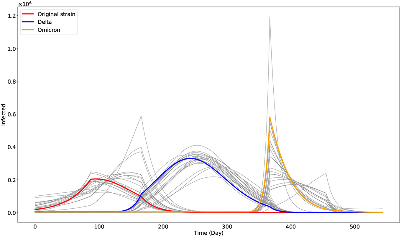
Figure 3. Plot of the three dominant COVID-19 variants in the Philippines as given by the model. The gray curves are the other outputs of the approximate Bayesian computation approach. The red, blue, and orange curves represent the best fit model output associated with the original strain (I₁), Delta (I₂), and Omicron (I₃) variants, respectively.

5.1. Deterministic simulations on waning vaccine-induced immunity

The Philippines started its vaccination campaign last 1 March 2021, with the two-dose Sinovac vaccine [26]. We estimated that it would need 4 weeks or 28 days to be fully protected from the vaccine [11], so we started the parameters ν and λ₁ by Day 87 (29 March 2021). It is estimated that the vaccine-induced immunity wanes after 6 months and that booster shots are recommended after that time interval [27]. Some people are unwilling to take booster shots due to vaccine hesitancy. Accounting for this social behavior in the model, we consider three different vaccine-induced immunity duration through the parameter λ₁ by setting it to 1/180 (6 months). This accounts for the case when the population only takes full vaccination but no booster shots. On the contrary, we set λ₁ = 1/365 (12 months) when the people finished taking the first booster shot, while λ₁ = 1/540 (18 months) when they completed the second booster shot. We simulate up to 31 December 2023 (Day 1094). The result is shown in Figure 4.

FIGURE 4

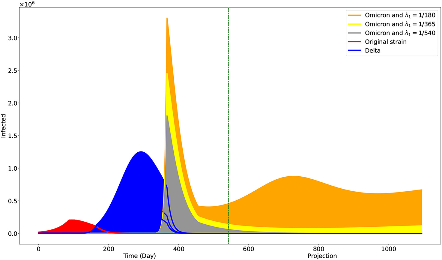
Figure 4. Projection on the effects of different levels of vaccine-induced immunity duration. The green vertical line is at Day 543, the end of the data used. One may interpret the case when λ₁ = 1/180 to be the case when individuals only opt to be fully vaccinated. The cases λ₁ = 1/365 and λ₁ = 1/540 may correspond to the cases when individuals are also getting first and second booster shots, respectively.

5.2. Stochastic simulations on the dominant transmission rate

As shown in Figure 4, our simulation suggested that the original and Delta variants are to die out even with the minimum vaccine-induced immunity duration of 6 months. But it is not the case with regard to the Omicron variant. However, we acknowledge that much uncertainty can affect the reduced transmission rate αβ₃—for instance, the changing control measures of the government and the further evolution of the variant. Hence, we also want simulations incorporating noise on αβ₃. In Figure 5, we show the result of our stochastic simulations. The curves are for the confirmed compartment. The figure can be viewed as a 3 × 2 matrix where the rows correspond to the cases corresponding to the different vaccine-induced immunity duration, given by the value of λ₁. The columns show the results concerning different noise intensities, given by the value of σ. The stochastic simulations start after Day 543 and run up to 31 December 2023 (Day 1094). The numerical simulations are implemented using the Euler–Maruyama scheme [28].

FIGURE 5

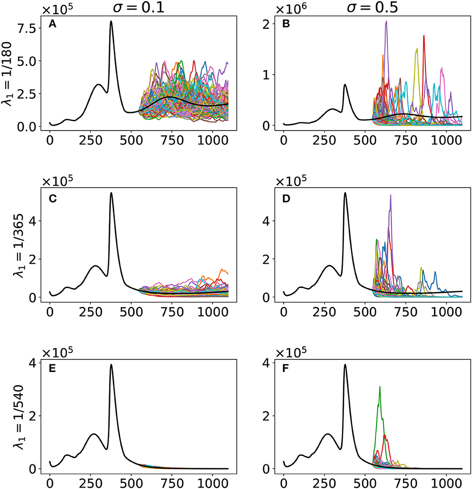
Figure 5. Stochastic simulations with respect to the vaccine-induced immunity duration λ₁ and noise intensity σ. The curves are for the confirmed compartment. The black curve is the deterministic model output, while the colored curves are the realizations of the 100 runs of the stochastic model. The cases are as follows: (A) λ₁ = 1/180, σ = 0.1; (B) λ₁ = 1/180, σ = 0.5; (C) λ₁ = 1/365, σ = 0.1; (D) λ₁ = 1/365, σ = 0.5; (E) λ₁ = 1/540, σ = 0.1; (F) λ₁ = 1/540, σ = 0.5.

6. Discussion

With our deterministic model, we have obtained parameters fitting observed data on confirmed cases in the Philippines. Our model has the added value that it could estimate the progression of the three main variants circulating the Philippines. Our simulations showed that the Omicron variant would be the dominant variant as we advance and the other variants die out (Figure 4). Moreover, it showed the significantly faster transmission of the Omicron variant compared with the other two, as reported [29] and validated by some studies [30, 31]. Our population is a closed model, and Theorem 3.1 showed that the Omicron variant would eventually die out. However, the time of its realization depends on the vaccine-induced immunity duration. With a duration of approximately 6 months, the simulation shows a noticeable presence of the Omicron variant by 31 December 2023. However, this presence is reduced significantly with vaccine-induced immunity durations of 12–18 months. We note that these vaccine-induced immunity durations can be achieved with booster shots in the population. Looking at the effective reproduction number given in (13), by Day 543 and vaccine-induced immunity duration of 6 months, we have ${{R}}_1^e=0.1731$, ${{R}}_2^e=0.3463$, and ${{R}}_3^e=1.0390$. By Day 5000, we only have ${{R}}_3^e=0.9998$. However, with a vaccine-induced immunity duration of 12 months and at Day 543, we already have ${{R}}_3^e=0.5124$.

We acknowledge that a lot of changes can happen in the future. For instance, the ongoing evolution of the virus and the ever-changing control measures being implemented by the government. Hence, incorporating these uncertainties in our simulations can prove beneficial. Our stochastic simulations (Figure 5) reveal that uncertainties, represented as noise in our model, can significantly affect future outcomes when vaccine-induced immunity duration is only 6 months, as seen in the spread of the stochastic model output. An increase in vaccine-induced immunity duration means a decrease in the variability of our model output and hence better projection. The government can then use better projection to design more robust and refined intervention strategies to control the virus effectively.

Data availability statement

Publicly available datasets were analyzed in this study. This data can be found here: https://github.com/CSSEGISandData/COVID-19.

Author contributions

RC-a and JA conceptualized the paper and drafted the manuscript. HC, MR, and RC-a did the mathematical analysis. JM did the biological part. RC-a performed the simulations. All authors contributed to manuscript revision, read, and approved the submitted version.

Funding

This project was funded by the Philippines' Department of Science and Technology – Philippine Council for Health Research and Development, MSU – Iligan Institute of Technology's Office of the Vice-Chancellor for Research and Extension through the Premier Research Institute of Science and Mathematics, and the Caraga State University Mathematical, Statistical & Computing Research Center.

Conflict of interest

The authors declare that the research was conducted in the absence of any commercial or financial relationships that could be construed as a potential conflict of interest.

Publisher's note

All claims expressed in this article are solely those of the authors and do not necessarily represent those of their affiliated organizations, or those of the publisher, the editors and the reviewers. Any product that may be evaluated in this article, or claim that may be made by its manufacturer, is not guaranteed or endorsed by the publisher.

References

1. Zhu N, Zhang D, Wang W, Li X, Yang B, Song J, et al. A novel coronavirus from patients with pneumonia in China, 2019. N Engl J Med. (2020) 382:727–33. doi: 10.1056/NEJMoa2001017

PubMed Abstract | CrossRef Full Text | Google Scholar

2. World Health Organization. Tracking SARS-CoV-2 Variants (2022). Retrieved from: https://www.who.int/activities/tracking-SARS-CoV-2-variants

3. The World Bank. Reducing Vaccine Hesitancy in the Philippines: Findings from a Survey Experiment (2021). Retrieved from: https://thedocs.worldbank.org/en/doc/9b206c064482a4fbb880ee23d6081d52-0070062021/original/Vaccine-Hesitancy-World-Bank-Policy-Note-September-2021.pdf

Google Scholar

4. World Health Organization. Donors Making a Difference: Knocking Down Obstacles to COVID-19 Vaccination (2022). Retrieved from: https://www.who.int/news-room/feature-stories/detail/donors-making-a-difference-knocking-down-obstacles-to-covid-19-vaccination

5. Arcede JP, Caga-anan RL, Mentuda CQ, Mammeri Y. Accounting for symptomatic and asymptomatic in a SEIR-type model of COVID-19. Math Modell Nat Phenomena. (2020) 15:34. doi: 10.1051/mmnp/2020021

CrossRef Full Text | Google Scholar

6. Macalisang JM, Caay ML, Arcede JP, Caga-anan RL. Optimal control for a COVID-19 model accounting for symptomatic and asymptomatic. Comput Math Biophys. (2020) 8:168–79. doi: 10.1515/cmb-2020-0109

PubMed Abstract | CrossRef Full Text | Google Scholar

7. Bock W, Bornales JB, Burgard JP, Babiera JE, Caga-anan RL, Carmen DJS, et al. Testing, social distancing and age specific quarantine for COVID-19: case studies in Iligan City and Cagayan de Oro City, Philippines. In: AIP Conference Proceedings. AIP Publishing LLC (2020). doi: 10.1063/5.0029818

CrossRef Full Text | Google Scholar

8. Arcede JP, Caga-anan RL, Mammeri Y, Namoco RA, Gonzales ICA, Lachica ZP, et al. A modeling strategy for novel pandemics using monitoring data: the case of early COVID-19 pandemic in Northern Mindanao, Philippines. SciEnggJ. (2022) 15, 35–46.

Google Scholar

9. Arcede JP, Basañez RC, Mammeri Y. Hybrid modeling of COVID-19 spatial propagation over an Island Country. In: Advances in Computational Modeling and Simulation. Singapore: Springer (2022). p. 75–83.

Google Scholar

10. Estadilla CDS, Uyheng J, de Lara-Tuprio EP, Teng TR, Macalalag JMR, Estuar MRJE. Impact of vaccine supplies and delays on optimal control of the COVID-19 pandemic: mapping interventions for the Philippines. Infect Dis Poverty. (2021) 10:46–59. doi: 10.1186/s40249-021-00886-5

PubMed Abstract | CrossRef Full Text | Google Scholar

11. Caga-anan RL, Raza MN, Labrador GSG, Metillo EB, del Castillo P, Mammeri Y. Effect of vaccination to COVID-19 disease progression and herd immunity. Comput Math Biophys. (2021) 9:262–72. doi: 10.1515/cmb-2020-0127

CrossRef Full Text | Google Scholar

12. Cabanilla KI, Enriquez EAT, Velasco AC, Mendoza VMP, Mendoza R. Optimal selection of COVID-19 vaccination sites in the Philippines at the municipal level. PeerJ. (2022) 10:e14151. doi: 10.7717/peerj.14151

PubMed Abstract | CrossRef Full Text | Google Scholar

13. Buhat CAH, Duero JCC, Felix EFO, Rabajante JF, Mamplata JB. Optimal allocation of COVID-19 test kits among accredited testing centers in the Philippines. J Healthcare Inform Res. (2021) 5:54–69. doi: 10.1007/s41666-020-00081-5

PubMed Abstract | CrossRef Full Text | Google Scholar

14. Diekmann O, Heesterbeek JAP, Metz JA. On the definition and the computation of the basic reproduction ratio R 0 in models for infectious diseases in heterogeneous populations. J Math Biol. (1990) 28:365–82. doi: 10.1007/BF00178324

PubMed Abstract | CrossRef Full Text | Google Scholar

15. Van den Driessche P, Watmough J. Reproduction numbers and sub-threshold endemic equilibria for compartmental models of disease transmission. Math Biosci. (2002) 180:29–48. doi: 10.1016/S0025-5564(02)00108-6

PubMed Abstract | CrossRef Full Text | Google Scholar

16. Dong E, Du H, Gardner L. An interactive web-based dashboard to track COVID-19 in real time. Lancet Inf Dis. (2020) 20:533–4. doi: 10.1016/S1473-3099(20)30120-1

PubMed Abstract | CrossRef Full Text | Google Scholar

17. American Society for Microbiology. How Dangerous Is the Delta Variant (B.1.617.2)? (2021). Retrieved from: https://asm.org/Articles/2021/July/How-Dangerous-is-the-Delta-Variant-B-1-617-2

18. Virginia Department of Health. Variants of the Virus that Causes COVID-19. Retrieved from: https://www.vdh.virginia.gov/coronavirus/get-the-facts/variants-of-covid

Google Scholar

19. DOH. National COVID-19 Vaccination Dashboard (2022). Retrieved from: https://doh.gov.ph/covid19-vaccination-dashboard

20. Shrestha NK, Burke PC, Nowacki AS, Terpeluk P, Gordon SM. Necessity of coronavirus disease 2019 (covid-19) vaccination in persons who have already had COVID-19. Clin Infect Dis. (2022) 75:e662–71. doi: 10.1093/cid/ciac022

PubMed Abstract | CrossRef Full Text | Google Scholar

21. DOH. COVID-19 Bulletin # 293 (2022). Retrieved from: https://doh.gov.ph/covid19casebulletin293

22. Philippine Statistics Authority. Retrieved from: https://psa.gov.ph/content/2020-census-population-and-housing-2020-cph-population-counts-declared-official-president

23. Csilléry K, Blum MG, Gaggiotti OE, Francois O. Approximate Bayesian computation (ABC) in practice. Trends Ecol Evol. (2010) 25:410–8. doi: 10.1016/j.tree.2010.04.001

PubMed Abstract | CrossRef Full Text | Google Scholar

24. Levenberg K. A method for the solution of certain non-linear problems in least squares. Q Appl Math. (1944) 2:164–8. doi: 10.1090/qam/10666

CrossRef Full Text | Google Scholar

25. Marquardt DW. An algorithm for least-squares estimation of nonlinear parameters. J Soc Indus Appl Math. (1963) 11:431–41. doi: 10.1137/0111030

CrossRef Full Text | Google Scholar

26. Parrocha A. PH Kick-Starts COVID-19 Vaccination Drive with CoronaVac. Philippine News Agency (2021). Retrieved from: https://www.pna.gov.ph/articles/1132127

27. World Health Organization. Interim Statement on the Use of Additional Booster Doses of Emergency Use Listed mRNA Vaccines Against COVID-19 (2022). Retrieved from: https://www.who.int/news/item/17-05-2022-interim-statement-on-the-use-of-additional-booster-doses-of-emergency-use-listed-mrna-vaccines-against-covid-19

28. Kloeden PE, Platen E. Stochastic differential equations. In: Numerical Solution of Stochastic Differential Equations. Berlin; Heidelberg: Springer (1992). p. 103–60 doi: 10.1007/978-3-662-12616-5_4

CrossRef Full Text | Google Scholar

29. World Health Organization. One Year Since the Emergence of COVID-19 Virus Variant Omicron (2022). Retrieved from: https://www.who.int/news-room/feature-stories/detail/one-year-since-the-emergence-of-omicron

30. Ren SY, Wang WB, Gao RD, Zhou AM. Omicron variant (B. 1.1. 529) of SARS-CoV-2: mutation, infectivity, transmission, and vaccine resistance. World J Clin Cases. (2022) 10:1. doi: 10.12998/wjcc.v10.i1.1

PubMed Abstract | CrossRef Full Text | Google Scholar

31. Vitiello A, Ferrara F, Auti AM, Di Domenico M, Boccellino M. Advances in the omicron variant development. J Intern Med. (2022) 292:81–90. doi: 10.1111/joim.13478

PubMed Abstract | CrossRef Full Text | Google Scholar