 Sylvie Diane Djiomba Njankou
 Farai Nyabadza
- 1Department of Mathematics, University of Buea, Buea, Cameroon
- 2Department of Mathematics and Applied Mathematics, University of Johannesburg, Johannesburg, South Africa
Introduction: The good health of the economy of developed countries is an attracting factor for economic migrants from poorer countries whose movements can be associated with the spread of diseases such as the Ebola virus disease.
Methods: In this paper, we formulate a model of Ebola virus disease that considers two patches with different economic statuses represented by the respective gross-national incomes of the two patches. First, we consider a one-directional movement from a poorer patch to a rich patch. Second, we consider a two-way migration model where people move between patches.
Results: The steady states of the model are determined and analyzed. The analysis shows also that the disease free and the endemic equilibrium points are locally stable. The analysis also shows that a unique endemic equilibrium point exists in the poor patch when the reproduction number in this patch is greater than one and multiple endemic equilibria exist in the rich patch when the reproduction number in the poor patch is less than one. The model dynamics of the rich patch present a backward bifurcation which does not facilitate easy Ebola virus disease control. Sensitivity analysis is carried out to determine the most sensitive parameters that must be carefully estimated for the successful control of the Ebola virus disease.
Discussion: Numerical simulations indicate a decrease in the number of infected individuals in the rich patch when movements of populations are limited through the improvement of the economy in the poor patch. So, the improvement of the economy of poorer countries may be critical in avoiding potential outbreaks of Ebola virus disease.
1. Introduction
Ebola virus disease (EVD) is a serious hemorrhagic fever that is highly infectious and characterized by a high case fatality rate [1]. EVD has flu-like symptoms on its onset and progresses to vomiting, diarrhea, rash, and internal and external bleeding accompanied by impaired kidney and liver functions, which leads to death [2, 3]. The 2014-2016 EVD outbreak in West Africa saw 28,616 cases of EVD and 11,310 deaths in Guinea, Liberia, and Sierra Leone. The epidemic spread beyond the borders of the three countries with an additional 36 cases and 15 deaths occurring [4]. The most recent outbreaks were declared in the Democratic Republic of Congo (DRC), between 8 October to 16 December 2021 and 20 September 2022 in Uganda. There were 11 cases (eight confirmed, three probable) and the overall case fatality ratio (CFR) was 82% among total cases and 75% among confirmed cases in the DRC [5]. A total of 23 deaths, including five among confirmed patients (CFR among confirmed cases 28%), have been recorded from the districts of Mubende, Kyegegwa, and Kassanda as of September 25, 2022. There have also been a total of 18 confirmed cases and 18 probable cases reported [6].
Economic migration within the African continent is a reality, and it is more intense in West Africa in particular since the Economic Community of West African States effectively facilitates the free movement of people and goods (ECOWAS) [7]. Among the West African countries affected by EVD in 2013 − 2016, those with a higher GNI, as represented in Figure 1, are assumed to be economically more attractive. Meliandou is a village in Guinea considered as ground zero of EVD outbreak of 2013 − 2016. It is a triangular-shaped forested area where the borders of Guinea, Liberia and Sierra Leone converge [9]. Many unemployed people's search for employment causes population migrations to be erratic across borders that are incredibly permeable, which encourages the spread of a highly contagious illness like Ebola [9]. According to the WHO assessment, a factor that eventually developed into a significant driving force as the EVD outbreak spread was a very rapid movement of persons from communities across the border [9]. In addition, viruses can spread over great distances, and researchers assert that demographic changes made it difficult to manage EVD in West Africa [10, 11]. West African countries affected by the 2013 − 2016, EVD outbreak are classified as low income countries and are among the poorest in the world [8]. In Guinea, Liberia and Sierra Leone, the economic activity practiced by the majority of the population is informal whereas qualified jobs are practiced by few people [12–14]. Therefore, the transmission of the disease during the EVD pandemic was aided by population movements brought on by poverty.
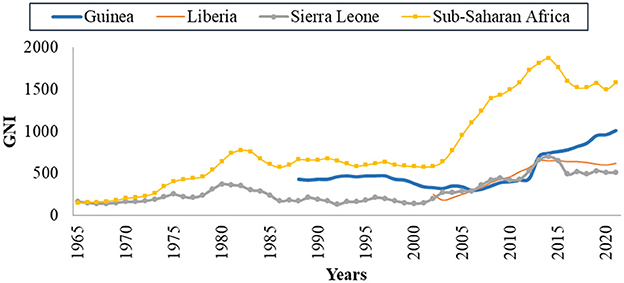
Figure 1. Annual per capita GNI in Africa, source [8].
2. Methods
Several mathematical models of EVD dynamics evaluate the impact of interventions on the disease dynamics or the spatial spread of the disease [7, 15–20]. Currently, there is no mathematical model linking EVD dynamics and the economic migration of populations, to the best of our knowledge. Countries affected by the outbreak of 2013 − 2016 are among the poorest in Africa as their per capita gross-national incomes GNI is very low when compared to the average on the continent [21]. Among the different tools used to measure the health of the economy of a country, such as the GDP (the Gross Domestic Product) and the GNI, we choose to use the GNI because it relates more to the income per individual in a country. It is also used to evaluate the impact of the economy on infectious diseases spread [22–24]. We observe in Figure 1 that the GNI in 2012 was increasing before the rise of EVD outbreak in the West African countries affected and started to decline after EVD hit these countries [25]. Data used to draw the graphs in Figure 1 were taken from World Bank [8] and data missing in the source are represented by empty spaces.
Movements between different socio-economic classes can result in the spread of an infectious disease such as EVD and the spatial spread of the disease is the immediate consequence of population mobility. Kiskowski and Chowell [26] modeled household and community transmission of EVD by employing a stochastic individual-level model. They assumed that control measures or behavior change could explain sub-exponential growth of EVD and concluded that greater epidemic control plus limited community mixing decrease the size of an infectious wave [26]. However, none of these models associated the economic status of the affected countries with the spatial spread of EVD, and our work is uniquely posed to address such an important observation.
The word income refers to the per capita GNI in this work. We consider that movements of individuals between two patches, from patch 2 to patch 1, are due to a lower income in patch 2 and a higher income in patch 1. We consider that when the income is close to zero in at least one patch, there is no movement of individuals. In fact, if the income in patch 2 is zero, people cannot afford to migrate since migration has a minimum cost, related to transport for example. If the income in patch 1 is zero, then the patch is not attractive economically. So, assuming that income decreases when the number of EVD infected individuals increases and based on the equation in Pluciński et al. [23] that links disease and income, we model the rate of change of income as
Where Mi is the per capita income in patch i, πi is the maximum income earned in the absence of EVD and ϵi is the half-saturation constant in patch i. We define ri (ri > 0) as the income growth rate per unit currency invested.
In this paper, we assume that the increasing number of EVD cases highly affected the economies of these countries and contributed to a decrease in income in general, see also African Union [12]. So, we choose to focus on the interaction between income and EVD and we study how they have impacted each other through human mobility. We first focus on a model for one-way economic migration and then we consider a two-way migration where migrants return to their country of origin for non-economic reasons. We aim to model the effect of low income on EVD dynamics through a one-way economic migration of populations, by assuming that the increasing number of EVD cases contributes to a decrease in the GNI of the affected countries. We also model a two-way migration model with the aim of evaluating the effects of the different scenarios on EVD dynamics in the two patches.
The work presented in this paper is arranged as follows: we first analyse the one-way migration model that is presented in Section 3. The two-way migration model is presented and analyzed in Section 4 and numerical simulations are presented in Section 5. The paper is concluded in Section 6.
3. One way migration model
The SEIRD Susceptible-Exposed-Infected-Recovered-Deceased model framework is used to model the economic migration of populations from a low-income country represented by patch 2 to a higher-income country represented by patch 1 and vice versa. Let i∈{1, 2} be the index of each considered patch. Susceptible individuals in patch i (Si), recruited at a rate Λi, get in contact with individuals infected by EVD (Ii) in the same patch and become exposed individuals (Ei). EVD transmission rate in patch i is βi which is the product of the number of contacts an individual in patch i can have multiplied by the probability for the contact to be infectious. After the incubation period in patch i, exposed individuals progress at a rate δi to become infected and are assumed not to recover or die from EVD at this stage. Infected individuals can either recover at a rate αi and join the recovered class Reci or may die because of the disease at a rate ϕi and join the compartment of the deceased Di. Bodies of the deceased are assumed to be infectious and buried at a rate ρi. Assuming that the income in patch 1 is higher than the one in patch 2, we assume that susceptible and recovered individuals move from patch 2 to patch 1 at a rate θ12 in order to earn more income and improve their living standards. Exposed individuals move from patch 2 to patch 1 at a rate σ12 which is different from θ12 with σ12 ≤ θ12. The difference is due to the disease status of the exposed that influences their probability of migrating. We also assume that visitors from patch 2 do not leave patch 1 during the modeling time. We also assume that in the total absence of income (M2 = M1 = 0), there is no movement of individuals between the patches (θ12 = σ12 = 0). In this case, the model in each patch is similar to the model developed and analyzed in Weitz et al. [27]. In this work, the force of infection in patch i is given by
Where βi is the transmission rate in patch i. The transmission rate is the product of the probability that contact can lead to EVD transmission and the number of contacts that an individual can have in a given patch.
The income-ratio m or GNI-ratio is the ratio of the income in patch 2 to the income in patch 1 M2/M1. During EVD outbreak of 2013 − 2016, which corresponds to the modeling time in this chapter, Sierra Leone and Guinea had the highest GNI among the three West African countries affected and represented then the most attractive countries economically.
We noted that the GNI-ratio did not vary that much during EVD outbreak of 2013 − 2016 as shown in Figure 2, plotted with data from World Bank [8]. So, we consider m as a constant during the modeling time with, 0 < m ≤ 1, since the income in patch 1 is assumed to be higher than the income in patch 2. The constant m may be viewed as the economic gap between the considered economies. Low values of m (close to zero) indicate two distant economies while higher values (close to one) indicate very close economies in terms of their GNI. Diseases or natural catastrophes that tend to impact the economy of a country affect the value of m. All the parameters used in the model and their descriptions are given in Table 1.
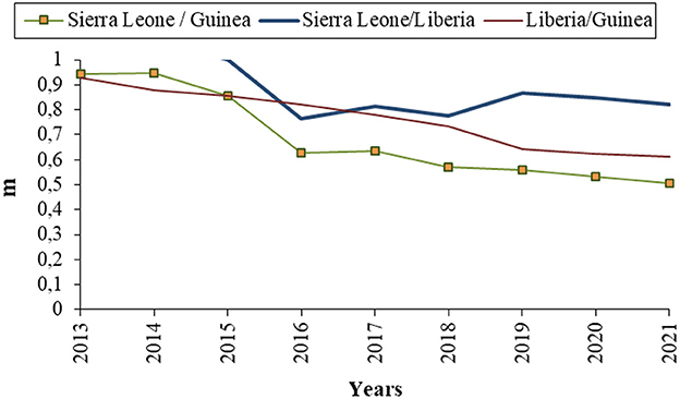
Figure 2. GNI-ratio of the countries affected by EVD in 2013 − 2016.
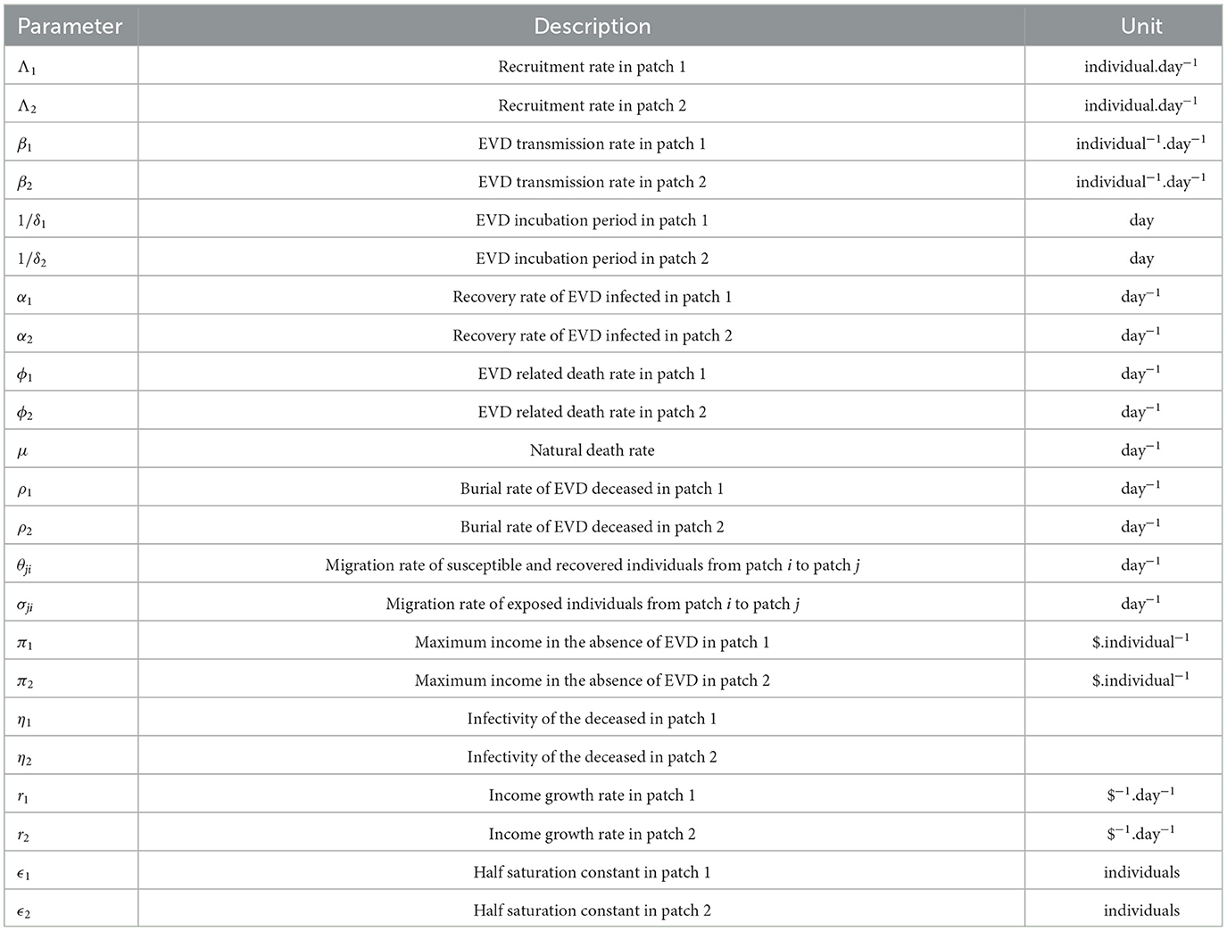
Table 1. Parameters' description for EVD economic migration model.
The one-way flow of individuals in the model is represented by Figure 3 and by the system of differential Equations (1)–(10).
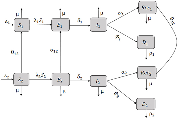
Figure 3. Flow chart diagram of EVD economic migration model.
Where Q1 = μ + δ1, Q2 = μ + δ2, Q3 = μ + α1 + ϕ1 and Q4 = μ + α2 + ϕ2. The initial conditions are:
Since the recovered individuals do not contribute to EVD transmission, their dynamics are decoupled from other variables in the closed system and their equation omitted.
3.1. Existence and positivity of solutions
Theorem 3.1. The invariant region is given by
where ,
,
Proof. We set H(t) = S(t) + E(t) + I(t). Adding Equations (1)–(6) yields
Using Gronwall inequality and integrating (Equation 11), we have
If , then the upper bound of H(t) is when t → ∞. If , then H(t) decreases to when t → ∞.
Then we obtain at infinity, .
Since for i = 1, 2, we obtain, respectively from Equations (7), (8)
resulting in the solutions and .
Since
from Equations (9), (10) we have
Solving the differential equations corresponding to Equations (15), (16) and applying Gronwall inequality yields
Theorem 3.2. All the solutions of the system (Equations 1–10) are non-negative for non-negative initial conditions.
Proof. Using Equation (1) and setting A1(t) = λ1(t) + μ, we obtain
Solving Equation (17) for all t ≥ 0 yields
So, S1(t) > 0 since S1(0) > 0. Similarly, we set A2(t) = λ2(t) + μ + θ12(1−m) and from Equation (2) we obtain
Equations (9), (10) imply
since for i = 1, 2.
Applying Gronwall inequality to Equations (18), (19) yields and . So, M1 and M2 are positive provided M1(0) and M2(0) are positive.
System Equation (3)–(8) can be rewritten as where
with
Since all the off-diagonal elements of T are non-negative, T is a Metzler matrix and G is monotone and positive, see Bokharaie [28]. So, is invariant under and G(t) is non-negative.
Finally, E1, E2, I1, I2, D1, D2 are non-negative and we can conclude that all the solutions of the system (Equation 1–10) are non-negative.
3.2. Disease free equilibrium
The disease free equilibrium (DFE) is given by where
By using the next generation matrix method to compute the reproduction number R0 of the system Equations (1)–(10), we obtain
where
R1 is the reproduction number in patch 1 and R2 is the reproduction number in patch 2. The stability of the DFE for a multi-city compartmental model is extensively discussed by Van Den Driessche and Arino in Arino and Van Den Driessche [29] so that we have the following result
Theorem 3.3. The DFE of system (Equations 1–10) is locally asymptotically stable whenever R0 < 1 and unstable otherwise.
3.3. Endemic equilibrium
The endemic equilibrium is given by:
where
is a positive solution of the polynomial (Equation 2). By replacing all the state variables in Equation (1) by their expressions at equilibrium from system (Equation 20), we obtain,
Where
where
,
Theorem 3.4. Polynomial (Equation 21) admits:
(i) One positive root if R2 > 1,
(ii) Zero or two positive roots if R2 < 1.
Proof. Descartes' Law of signs helps to determine the number of positive roots of polynomial (Equation 21). We count the number of sign changes of the coefficients of the polynomial and the value obtained is the maximum number of positive roots of the polynomial. The coefficient a0 is always positive. The coefficient a2 is positive when R2 < 1 and negative when R2 > 1. The maximum number of sign changes of the coefficients of the polynomial (Equation 21) is 2 if a1 < 0 and zero if a1 > 0 when R2 < 1. When R2 > 1, the maximum number of sign changes of the polynomial (Equation 21) is one.
From Equation 21, we can say that R2 > 1 guarantees the existence of a unique endemic equilibrium point in patch 2 so that and co-exist in this case. When R2 < 1 there is no endemic equilibrium point in patch 2 whereas up to two positive values of can exist. In this case, controlling EVD in patch 1 is then more complex as multiple endemic equilibria could exist. So, the existence of positive values of relies more on values of R2 and not on values of R1 as we could have expected. In fact, movements of exposed individuals from patch 2 to patch 1 continuously feed patch 1 with exposed individuals that later become infectious. So, whether there are secondary infections in patch 1 or not, movements of exposed individuals into this patch guarantees always the existence of an endemic equilibrium. EVD control in patch 1 should then first target immigration's control and its consequences.
We notice that in the absence of movements of exposed individuals (σ12 = 0), polynomial (21) becomes
and admits a unique positive root with
Theorem 3.5. The endemic equilibrium E* exists when R2 > 1 and is locally asymptotically stable.
Proof. The jacobian matrix of system (Equations 1–10) at the endemic equilibrium is given by
where
0i×j is the zero matrix of order i, j with
From Equations (9), (10), we obtain at equilibrium
Using Equations (22), (23) to simplify ψ7 and ψ9 yields
and
Since is a block triangular matrix, its diagonal entries are its eigenvalues. Since all the diagonal entries of the matrix are negative, we can conclude that all the eigenvalues of are negative and the endemic equilibrium E* is locally asymptotically stable.
3.4. Bifurcation analysis
A change of the topological structure of a system is called bifurcation [30] which is discussed in Ogunmilovo and Idowu [31]. A bifurcation driven by R2 is illustrated in Figure 4.
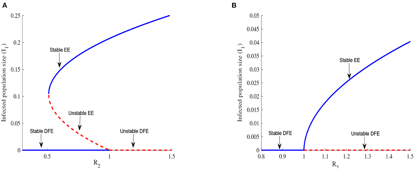
Figure 4. Backward bifurcation in (A) for Λ1 = 6270, Λ2 = 5370, β1 = 0.525, β2 = 0.385, α1 = 0.283, α2 = 0.394, ϕ1 = 0.304, ϕ2 = 0.373, ρ1 = 0.738, ρ2 = 0.637, η1 = 2.78, η2 = 2.81, , , μ = 0.048, θ12 = 0.277, σ12 = 0.637, m = 0.7. Forward bifurcation in (B) for m = 0.982.
Figures 4A, B illustrate the possible number of positive roots of the polynomial (Equation 21) when R2 is varied. A backward bifurcation is observed in Figure 4A when R2 < 1 and a forward bifurcation is observed in Figure 4B when R2 > 1. The complexity of the system of Equations (1)–(10) makes it difficult to prove the existence of The backward bifurcation but we can observe it thanks to numerical simulations.
The backward bifurcation shows a locally stable DFE and an unstable EE. In any disease control, reaching a globally stable DFE is the main target, but this is more difficult to realize in the case of a backward bifurcation since the DFE is globally stable only below a threshold , whose value might be far from 1. The expression of Rt is obtained by setting to zero the discriminant of the polynomial (Equation 21). The forward bifurcation represented in Figure 4B offers an easier possibility because reducing R2 to values less than one is enough in this case to reach a globally stable DFE and is then the preferable scenario for EVD control.
The income ratio describes the gap between two economies and this gap is considered the main driving factor of migration in this work. We observe in Figure 4 that a backward bifurcation is changed into a forward bifurcation for the chosen parameter values when the value of m is increased. Increasing the value of m corresponds to bringing closer the two economies considered and this can be done by increasing the per capita income in patch 2 for example. This increase in income certainly improves the living condition of people in this patch and reduces their chances of migrating. EVD control becomes easier in this case as exposed individuals can be easily tracked and isolated in both patches. Improving the economy of poor countries exposed to EVD in order to stop or limit the migration of individuals exposed to the disease is a useful measure to be implemented by all governments, especially governments of rich countries because the migration of infected individuals might cause an EVD outbreak in their countries.
4. Two way migration
Some economic migrants return for some time to their home countries. These returns are sometimes due to one of the following reasons: the migrants couldn't find a job in the host country, they have simply realized that the reality of the host country does not meet their initial expectations or they return to visit their families. Migrants transfer savings, education, and skills to their home country when they return after a stay in a more developed country [32]. We assume in this case a two-way migration of populations for which susceptible migrants from patch 1 return to patch 2 at the rate θ21 and exposed migrants return at a rate σ21 after a stay in patch 1. The flow chart diagram representing the two ways migration is given in Figure 5.
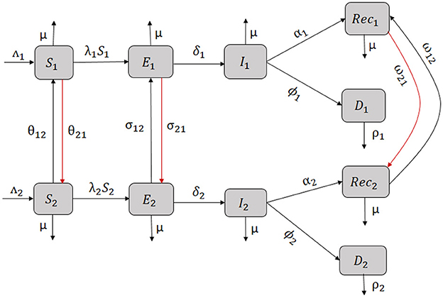
Figure 5. Flow chart diagram of the two-way migration model.
Solutions of the system (Equations 24–33) exist and are positive and the proof follows the proof of Theorem 3.1.
At DFE, where
The next generation matrix method [33] is used to compute the reproduction number which is the largest eigenvalue of the product where Fg is the renewal matrix and Vg is the transfer matrix.
We set where aij = 0 ∀i, j∈{1, …, 6}, except
where and .
The reproduction number in this case is
where with
Since aij ≥ 0 ∀i, j, and the reproduction number is .
The endemic equilibrium is given by
where
and are the positive solutions of the system of Equation 35 obtained by substituting the values of the state variables from system (Equations 24, 25, 34).
where
The complexity of the resolution of system (Equation 35) does not enable us to give explicit expressions for and and this does not facilitate the study of the stability of equilibria. However, the use of the next generation matrix method to compute the reproduction number guarantees at least the local stability of [33]. We now resort to numerical simulations to study the system further.
5. Numerical simulations
We simulate a scenario where susceptible and exposed individuals from a given community in Liberia move to Sierra Leone, based on the fact that since 1990, the GNI of Sierra Leone has always been larger than that of Liberia. The values of the parameters we use are either from the literature or estimated (deduced from the disease epidemiology and information on population mouvements) and are given in Tables 2, 3.
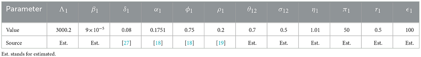
Table 2. Parameters with index 1 are for Sierra Leone.
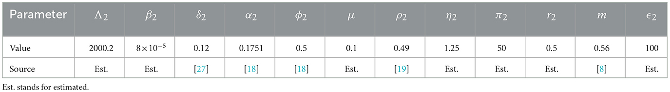
Table 3. Parameters with index 2 are for Liberia.
5.1. Sensitivity analysis
Some parameters are more influential than others and can be estimated through sensitivity analysis. Among all the existing techniques of sensitivity analysis, the Latin Hypercube Sampling (LHS) and Partial Rank Correlation Coefficient (PRCC), LHS/PRCC sensitivity analysis presents the advantage of sampling the parameters independently of one another [34]. The objective of the LHS/PRCC sensitivity analysis is to determine and rank important parameters whose uncertainties increase prediction imprecision. For a given parameter, the LHS procedure consists of dividing the parameter values range into equally probable intervals and assigning a probability distribution to each parameter [34]. The PRCC that describes the linear relationship between the LHS parameters and the outcome measure is a statistical technique used to measure the strength of the relationship between the outcome measures and the parameters in a model [34].
EVD dynamics is well described by the variation in the number of infected individuals. But, since some of the parameter values used are estimated, there is some uncertainty in the results obtained and we use LHS/PRCC sensitivity analysis to identify key parameters that increase imprecision in the results obtained from system (Equations 1–10).
The reproduction number of system (Equations 1–10) is the largest of the two reproduction numbers in the two patches. Figure 6 represents the type and importance of the correlation between each reproduction number and the parameters of the model. We observe in Figure 6A that β1, ϕ1, η1 and σ12 have a positive correlation to R1 whereas α1, μ, ρ1 and m have a negative correlation to R1. β1, ϕ1, η1 are the components of EVD force of infection in patch 1. Therefore, they drive EVD spread in patch 1 and then have a positive correlation with R1. σ12 describes movements of exposed individuals into patch 1 who become later infectious, increasing then the number of infected individuals into the patch and this explains the positive correlation with R1. The natural death rate, recovery rate, and safe burials rate (considered as dead bodies disposal rate) respectively represented by α1, μ, ρ1 in patch 1, reduce the number of individuals susceptible to EVD and therefore reduce R1. This explains the negative correlation between these parameters and R1. Increasing the value of m corresponds to reducing the economy of patch 1. In the case of a poor economy in patch 1, fewer people will move to patch 1, limiting the number of people susceptible to EVD in patch 1 and this will then decrease R1. This explains the negative correlation between m and R1. Similarly, the results observed in Figure 6B represent the sensitivity analysis in patch 2, with the difference being that m has a positive correlation to R2 and σ12 has a negative correlation to R2. In fact, the movement of infected individuals from patch 2 reduces the infected population size and as a consequence, the reproduction number R2 is reduced as well. m has a positive correlation to R2 because increasing the value of m in patch 2 corresponds to improving the economy in this patch which results in fewer people leaving the patch. This increases the size of the population susceptible to contract EVD in patch 2 and as a consequence, the reproduction number R2 is increased. Key parameters whose uncertainty in the estimation of their values, might lead to imprecision in the results of the model analysis are then identified and represent a very important reserve of information for EVD control in this case. The estimation of these parameter values must then be carefully done during the formulation and implementation of control measures against EVD spread.
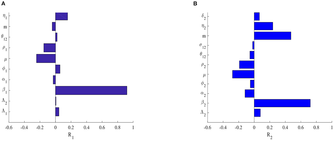
Figure 6. Sensitivity plots of the reproduction number in patch 1 in (A) and in patch 2 in (B) for the one-way migration model.
5.2. Dynamics of the infected individuals
The evolution of the number of infected individuals is represented in Figure 7.
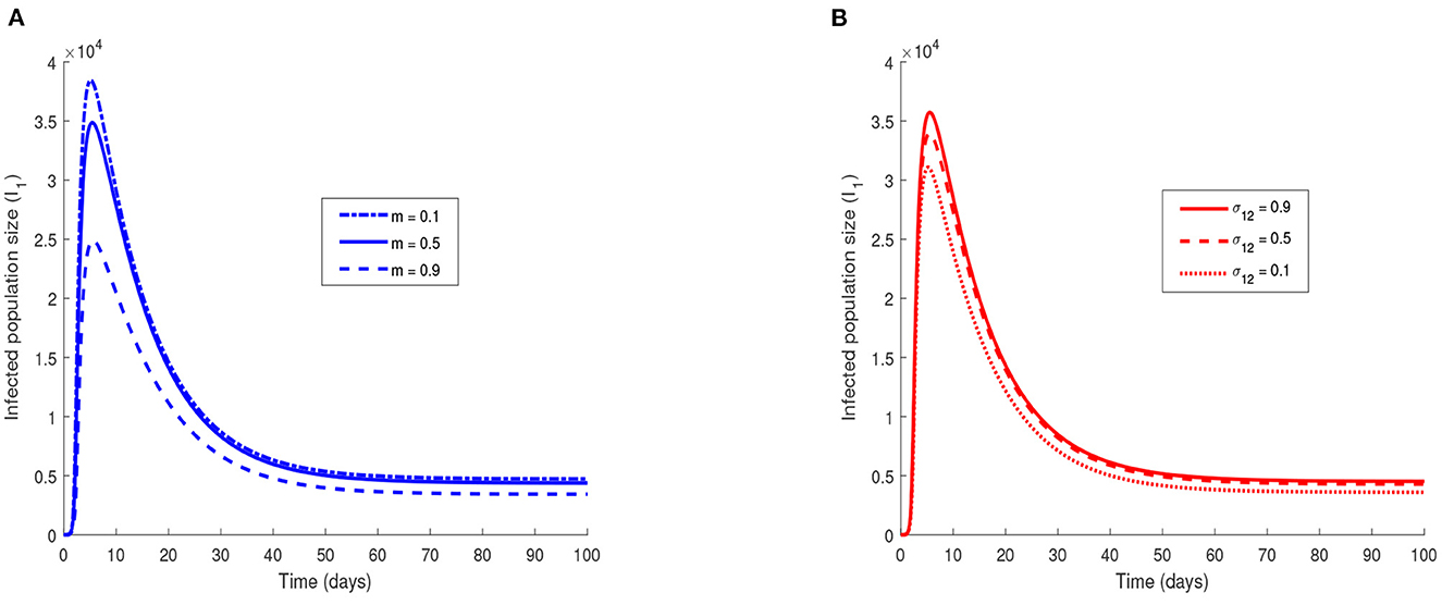
Figure 7. Effect of migration of infected individuals on EVD dynamics for the one-way migration model. Effect of migration of infected individuals on EVD dynamics in the case of a two-way migration. In (A) the income ratio is varied and in (B) the migration rate of exposed individuals is varied. The value of the parameters used are in Tables 2, 3. The initial conditions are S1(0) = S2(0) = 2, 000, I1(0) = I2(0) = 2.
Figure 7A shows an increase in the number of infected individuals in patch 1 when the value of m is decreased. A reduction of the income ratio m corresponds to an increase in the gap between the economies of the two considered patches or communities. This decrease can either be due to an increase of the GNI in patch 1 or a decrease of the GNI in patch 2. In both cases, the immediate consequence is that more individuals leave patch 2 for patch 1 either because the economy of their residing country is worse or because there are better opportunities elsewhere. Figure 7B confirms this hypothesis since we observe an increase in the number of infected individuals in patch 1 when the value of σ12 is increased. The economies of countries that can be potentially affected by EVD must then be very close in order to avoid the movements of individuals toward the rich countries. This economic migration in fact can import the Ebola virus into a country and can potentially cause an outbreak.
In the case of a two-way migration, we notice in Figure 8 that the size of the infected population is smaller when compared to Figure 7B where migration is only one way. Migration of populations from rich countries returning to their country of origin helps in EVD control in the rich country as it limits the number of EVD-infected individuals. Although these returns are not motivated by the improvement of the economic situation of the country of origin, it represents a better scenario for the rich country. It affirms the necessity for rich countries to facilitate more returning residents by providing those who want to return with entrepreneurial skills and funds to start their own businesses as they arrive at their country of origin for example. It might also be viewed as a call to facilitate the flow between countries through easy visa procedures for example.
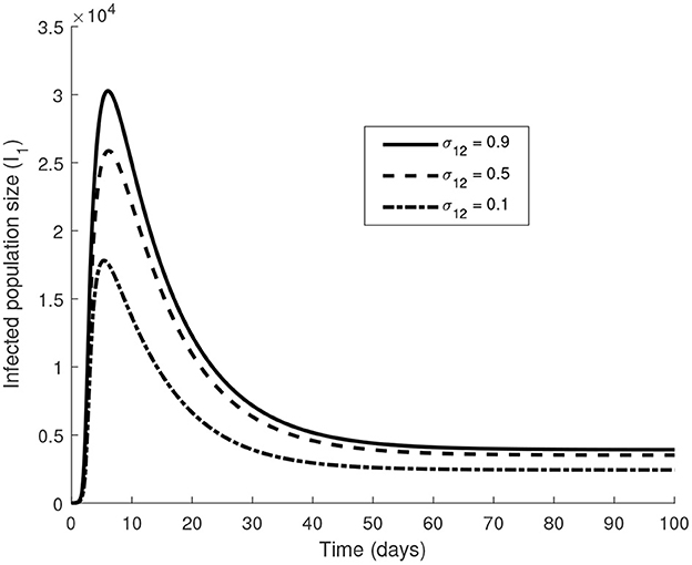
Figure 8. The value of the parameters used are in Tables 2, 3 with θ21 = 0.7 and σ21 = 0.5 The initial conditions are S1(0) = S2(0) = 2, 000, I1(0) = I2(0) = 2.
6. Conclusion
Economic migration has always been a way of improving some people's living conditions. Migration from Africa to Europe is the most advertised route for economic migrants, who sometimes illegally enter Europe through Italy [35]. Intra-African economic migration is less advertised, although free movements of persons and goods that facilitate such type of migration is a reality in some regions of the continent [7]. The health status of migrants is often unknown or not well documented and they can, therefore, possibly transport a virus to different geographical locations [36]. We formulated in this chapter, a model of EVD with two patches, that first considers the economic migration of individuals from patch 2 to patch 1, whose economy is assumed to be better, and second, we also consider the returning of migrants to patch 2. We chose the GNI to represent the economy in each patch and we used the income ratio, which is the ratio of the lowest economy to the highest economy, to represent the gap between two economies.
First, we proved that the one-way migration model makes biological sense in an invariant set. We found that the reproduction number of the system is the largest reproduction number of the two patches and the disease free equilibrium of the system is locally stable when the reproduction number is less than one. We found that there exists a unique endemic equilibrium point in patch 2 when R2 > 1 and there is a possibility of having multiple endemic equilibria in patch 1. The multiplicity of equilibrium points characterizes a bifurcation which, in this case, is backward when R2 < 1 and forward when R2 > 1. We found from the bifurcation analysis that improving the economy in patch 2 limits the movements of infected individuals and facilitates EVD control Second, we considered that migrants also return to their countries of departure and this changed the first model into a two-way migration model which presented a locally stable disease free equilibrium.
We simulated a scenario where individuals from a community in Liberia move to Sierra Leone whose economy is better as an example of the one-way migration model. We found the most sensitive parameters of the model by using LHS/PRCC sensitivity analysis and results from the numerical simulations show that limiting the migration of infected individuals into patch 1 by improving the economy of patch 2 contributes to a reduction of the number of EVD cases in patch 1. Rich countries are then not completely in the shadow of EVD since the good health of their economy attracts individuals from poorer countries, who might bring with them the Ebola virus. Since the scenario of all migrants at the borders of a country is very difficult to achieve, we suggest that poor countries improve the living conditions of their populations, for example by abolishing corruption that deprives its population of their wealth. We also suggest that developed countries contribute to the development of the poorest countries in order to avoid an invasion of EVD on their soils through economic migration. Simulations of the two-way model showed that fewer individuals are infected in the rich patch when some move to the poorer patch. The work presented in this chapter describes a scenario where EVD spread through economic migration, but it is not without shortcomings since other factors, other than economic conditions, motivate the migration of people. In fact, in the twenty-first century, political instability is a major cause of migration. People fleeing from conflict areas, which may be affected by infectious diseases, enter new areas of the terrestrial globe with a chance of spreading infectious diseases on their arrival. It will then be of great interest to assess the impact of such movements on the health of countries receiving refugees so as to raise awareness against war and other forms of conflict that are often the drivers of migration. The income ratio m is constant in this paper, but this value is also time-dependent and can therefore be modeled as m(t) in the future.
Data availability statement
The original contributions presented in the study are included in the article/supplementary material, further inquiries can be directed to the corresponding author.
Author contributions
FN supervised SN for her doctoral studies. Both formulated the model, SN analyzed and did simulations for the models. All authors reviewed the manuscript and contributed to the article and approved the submitted version.
Funding
This research was supported by the University of Johannesburg and the OWSD. The authors acknowledge the support of their respective institutions and OWSD in the production of the manuscript.
Acknowledgments
The authors also acknowledge that this paper is extracted from a dissertation [37].
Conflict of interest
The authors declare that the research was conducted in the absence of any commercial or financial relationships that could be construed as a potential conflict of interest.
Publisher's note
All claims expressed in this article are solely those of the authors and do not necessarily represent those of their affiliated organizations, or those of the publisher, the editors and the reviewers. Any product that may be evaluated in this article, or claim that may be made by its manufacturer, is not guaranteed or endorsed by the publisher.
References
1. WHO. Ebola Virus Disease (2022). Available online at: https://www.afro.who.int/health-topics/ebola-virus-disease (accessed on September 18, 2022).
2. Birmingham K, Cooney S. Ebola: small, but real progress. Nat Med. (2002) 8:313. doi: 10.1038/nm0402-313
3. WHO. Ebola Virus Disease (2022). Available online at: https://www.who.int/health-topics/ebola#tab=tab_1 (accessed on September 18, 2022).
4. CDC. 2014–2016 Ebola Outbreak in West Africa (2022). Available online at: https://www.cdc.gov/vhf/ebola/history/2014-2016-outbreak/index.html#:~:text=The%20impact%20this%20epidemic%20had,outside%20of%20these%20three%20countries (accessed on September 18, 2022).
5. DRC. Disease Outbreak News: Ebola virus Disease-Democratic Republic of the Congo (2021). Available online at: https://reliefweb.int/report/democratic-republic-congo/disease-outbreak-news-ebola-virus-disease-democratic-republic-3?gclid=Cj0KCQjw1bqZBhDXARIsANTjCPLt3AWIce8ihpUBmeQaqI-kMCuXpiTGq5hB3BTkX0y2qRk4jjWC5rykaAvNHEALw_wcB (accessed on September 18, 2022).
6. WHO. Ebola Disease caused by Sudan Virus-Uganda (2022). Available online at: https://www.who.int/emergencies/disease-outbreak-news/item/2022-DON410 (accessed on October 26, 2022).
7. Campbell L. Learning From the Ebola Response in cities: Population Movement (2022). Available online at: https://www.alnap.org/help-library/learning-from-the-ebola-response-in-cities-population-movement (accessed on October 15, 2022).
8. World Bank. Data (2022). Available online at: https://data.worldbank.org/indicator/NY.GNP.PCAP.CD (accessed on October 27, 2022).
9. WHO. Emergencies Preparedness, Response, Ebola at Six Months (2017). Available online at: http://www.who.int/csr/disease/ebola/ebola-6-months/guinea/en/ (accessed on November 1, 2017).
10. Shaw W. Migration in Africa : A Review of the Economic Literature on International Migration in 10 Countries (English). Washington, DC: World Bank Group (2022). Available online atL http://documents.worldbank.org/curated/en/248611468212384547/Migration-in-Africa-a-review-of-the-economic-literature-on-international-migration-in-10-countries (accessed on October 10, 2022).
11. Roos R. Migrations in West Africa Seen as Challenge to Stopping Ebola. CIDRAP News (2014). Available online at: cidrap.umn.edu/news-perspective/2014/11/migrations-west-africa-seen-challenge-stopping-ebola (accessed on December 15, 2016).
12. African Union. The Social Impact of Ebola in Particular the Nature of the Social Protection Interventions Required (2022). Available online at: https://au.int/sites/default/files/newsevents/workingdocuments/28072-wd-the_social_impact_of_ebola_-english.pdf (accessed on October 26, 2022).
13. Margolis D, Rosas N, Turay A, Turay S. Findings from the 2014 Labor Force Survey in Sierra Leone. World Bank (2016). doi: 10.1596/978-1-4648-0742-8
14. IMF Country Report No. 12/45. Liberia: Poverty Reduction Strategy Paper-Annual Progress Report (2012). Available online at: http://www.imf.org (accessed on October 27, 2022).
15. Bhunu CP, Mushayabasa S, Smith RJ. Assessing the effects of poverty in tuberculosis transmission dynamics. Appl Math Model. (2012) 36:4173–85. doi: 10.1016/j.apm.2011.11.046
16. Mushayabasa S, Bhunu CP, Webb C, Dhlamini C. A mathematical model for assessing the impact of poverty on yaws eradication. Appl Math Model. (2012) 36:1653–67. doi: 10.1016/j.apm.2011.09.022
17. Pedro SA, Tchuenche JM. HIV/AIDS dynamics: impact of economic classes with transmission from poor clinical settings. J Theor Biol. (2010) 267:471–85. doi: 10.1016/j.jtbi.2010.09.019
18. Upadhyay RK, Roy R. Deciphering dynamics of recent epidemic spread and outbreak in West Africa: the case of Ebola virus. Int J Bifurcat Chaos. (2016) 26:1630024. doi: 10.1142/S021812741630024X
19. Rivers CM, Lofgren ET, Marathe M, Eubank S, Lewis BL. Modelling the impact of interventions on an epidemic of Ebola in Sierra Leone and Liberia. PLoS Curr. (2014) 6:ecurrents.outbreaks.4d41fe5d6c05e9df30ddce33c66d084c. doi: 10.1371/2Fcurrents.outbreaks.4d41fe5d6c05e9df30ddce33c66d084c
20. Djiomba SD, Nyabadza F. An optimal control model for Ebola virus disease. J Biol Syst. (2016) 24:29–49. doi: 10.1142/S0218339016500029
21. The World Bank. Data, Sub-saharan Africa (2017). Available online at: http://data.worldbank.org/region/sub-saharan-africa (access on August 23, 2017).
22. IMF Country Report No. 13/191. Guinea: Poverty Reduction Strategy Paper (2018). Available online at: https://www.imf.org/en/Publications/CR/Issues/2016/12/31/Guinea-Poverty-Reduction-Strategy-Paper-40732 (accessed on December 10, 2018).
23. Pluciński MM, Ngonghala CN, Bonds MH. Health safety nets can break cycles of poverty and disease: a stochastic ecological model. J R Soc Interface. (2011) 8:1796–803. doi: 10.1098/2Frsif.2011.0153
24. Pluciński MM, Ngonghala CN, Getz WM, Bonds MH. Bonds. Clusters of poverty and disease emerge from feedbacks on an epidemiological network. J R Soc Interface. (2012) 10:20120656. doi: 10.1098/rsif.2012.0656
25. World Bank. The Economic Impact of the 2014 Ebola epidemic: Short and Medium-Term Estimates for West Africa (2014). Available online at: https://www.worldbank.org/en/region/afr/publication/the-economic-impact-of-the-2014-ebola-epidemic-short-and-medium-term-estimates-for-west-africa#:~:text=In%20the%20%E2%80%9CLow%20Ebola%E2%80%9D%20scenario,and%20%2425.2%20billion%20in%202015
26. Kiskowski M, Chowell G. Modelling household and community transmission of Ebola virus disease: epidemic growth, spatial dynamics and insights for epidemic control. Virulence. (2016) 7:163–173. doi: 10.1080/21505594.2015.1076613
27. Weitz JS, Dushoff J. Modeling post-death transmission of Ebola: challenges for inference and opportunities for control. Sci Rep. (2015) 5:8751. doi: 10.1038/srep08751
28. Bokharaie VS. Stability Analysis of Positive Systems With Application to Epidemiology. Sunnyvale, CA: LAP LAMBERT Academic Publishing (2012).
29. Arino J, Van Den Driessche P. The basic reproduction number in a multi-city compartmental epidemic model. In:Benvenuti L, De Santis A, Farina L, , editors. Positive systems. Lecture Notes in Control and Information Science, Vol. 294. Berlin; Heidelberg: Springer (2004). p. 135–42.
31. Ogunmilovo OM, Idowu AS. Bifurcation, sensitivity, and optimal control analysis of onchocerciasis disease transmission model with two groups of infectives and saturated treatment function. Math Methods Appl Sci. (2022) 2022:1–25. doi: 10.1002/mma.8317
32. Wahba J. Who benefits from return migration to developing countries? IZA World Labor (2021) 2021:123. doi: 10.15185/izawol.123.v2
33. Van Den Driessche P, Watmough J. Reproduction numbers and sub-threshold endemic equilibria for compartmental models of disease transmission. Math Biosci. (2002) 180:29–48. doi: 10.1016/S0025-5564(02)00108-6
34. Gomero B. Latin Hypercube Sampling Partial Rank Coefficient analysis applied to an optimal control problem (Master's thesis). University of Tennessee (2012). Available online at: https://trace.tennessee.edu/utk_gradthes/1278
35. Flahaux ML, De Haas H. African migration: trends, patterns, drivers. Comput Migr Stud. (2016) 4:1. doi: 10.1186/2Fs40878-015-0015-6
36. Rechel B. Migration and Health in the European Union. New York, NY: Open University Press; McGraw-Hill Education (2011).
Keywords: economic migration, Ebola, stability, reproduction number, bifurcation analysis, simulations
Citation: Diane Djiomba Njankou S and Nyabadza F (2023) Modeling the potential influence of economic migration on Ebola virus disease transmission dynamics. Front. Appl. Math. Stat. 9:1024571. doi: 10.3389/fams.2023.1024571
Received: 21 August 2022; Accepted: 13 February 2023;
Published: 28 February 2023.
Edited by:
Aurelio A. de los Reyes V, University of the Philippines Diliman, PhilippinesReviewed by:
Oluwatayo Michael Ogunmiloro, Ekiti State University, NigeriaVictoria May Mendoza, University of the Philippines Diliman, Philippines
Copyright © 2023 Diane Djiomba Njankou and Nyabadza. This is an open-access article distributed under the terms of the Creative Commons Attribution License (CC BY). The use, distribution or reproduction in other forums is permitted, provided the original author(s) and the copyright owner(s) are credited and that the original publication in this journal is cited, in accordance with accepted academic practice. No use, distribution or reproduction is permitted which does not comply with these terms.
*Correspondence: Sylvie Diane Djiomba Njankou,  c3lsdmllQGFpbXMtc2VuZWdhbC5vcmc=