Numerical solution of density-driven groundwater flows using a generalized finite difference method defined by an unweighted least-squares problem

Density-driven groundwater flows are described by nonlinear coupled differential equations. Due to its importance in engineering and earth science, several linearizations and semi-linearization schemes for approximating their solution have been proposed. Among the more efficient are the combinations of Newtonian iterations for the spatially discretized system obtained by either scalar homotopy methods, fictitious time methods, or meshless generalized finite difference method, with several implicit methods for the time integration. However, when these methods are used, some parameters need to be determined, in some cases, even manually. To overcome this problem, this paper presents a novel generalized finite differences scheme combined with an adaptive step-size method, which can be applied for solving the governing equations of interest on non-rectangular structured and unstructured grids. The proposed method is tested on the Henry and the Elder problems to verify the accuracy and the stability of the proposed numerical scheme.

1. Introduction

The study of density-driven groundwater flows is of special interest in groundwater hydraulics. That interest comes from the intrinsic relation that exists between density-driven groundwater problems, saltwater intrusion, and geothermal processes. Groundwater is used in many regions as the main available source to supply freshwater to their citizens and has become an increasingly valuable resource. Nowadays, seawater intrusion problems are crucial issues to pay more attention to, especially in coastal areas.

There are two important benchmark problems to test numerical methods in the resolution of density-driven groundwater flow problems, these are the Henry problem [1–7] and the Elder problem [4–6, 8]. The Henry problem is commonly used for describing salt concentration transport into a freshwater aquifer where the transport mechanism is because of fluid, while the Elder problem is frequently employed for describing natural geothermal convection problems.

Since both problems are coupled and highly nonlinear, the development of efficient, accurate, reliable, and simple numerical schemes developed to solve them remains a challenging task.

The Henry problem is named after Henry [1], who was studying salt concentration problems. He considered a vertical rectangular slice of a confined coast aquifer from which he obtained the boundary conditions (Figure 1) and developed a semi-analytical solution for the steady-state problem. He assumed a double Fourier series solution, which, after substitution into the governing equations and integration over the entire domain relative to ad hoc weight functions, gives rise to an infinite system of algebraic equations. Truncation of this system and solving for Fourier coefficients leads to the semi-analytical solution of the problem. A similar approach was presented in [9], where the Henry semi-analytical solution was obtained by considering reduced dispersion.

FIGURE 1

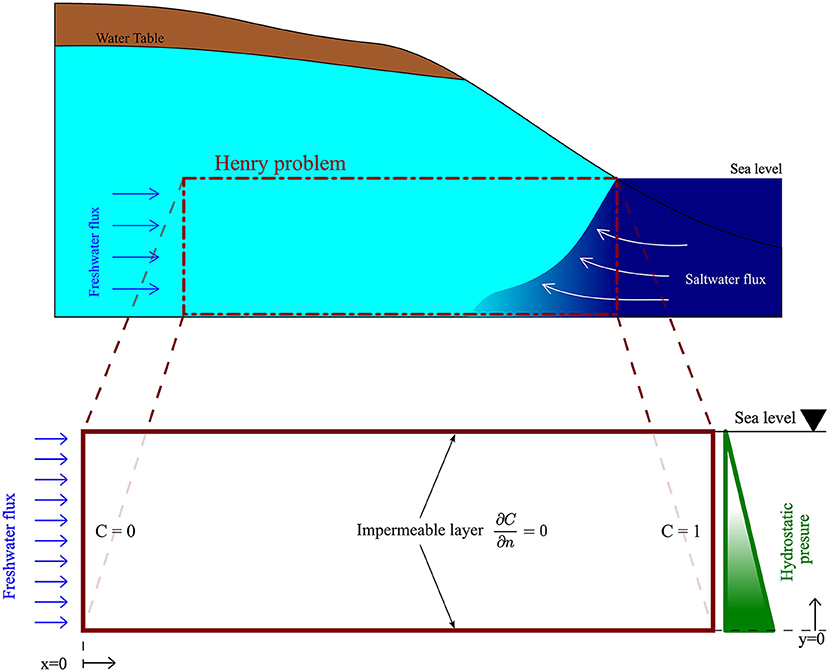
Figure 1. Henry problem computational domain.

Pinder and Cooper [2] obtained a semi-analytical solution for the transient formulation of the Henry problem using the method of characteristics, then considered two different initial conditions. In the first one, the aquifer was assumed to be fulfilled initially with fresh water, in the second condition a sharp interface into the aquifer was assumed initially.

Segol et al. [3] used the Galerkin-finite element method to solve the Henry problem. They obtained two solutions using two different meshes, the first one with 108 nodal points and 88 elements using linear basis functions, the second with 107 nodal points and 28 elements using quadratic basis functions. Their results are similar to other approaches in the aquifer domain but differ in the zone near the right boundary where a boundary modification is required.

Simpson and Clement [10] solved the Henry problem using the assumption of a double Fourier series solution and considering a quadratic term involving a quadruple sum as a known quantity. One feature of their solution is an iterative change of a boundary condition at the right side of the domain, which is transformed from a mixed Dirichlet-Neumann boundary condition to a Dirichlet one. This was the key to getting the problem of interest at the end.

The Elder problem is named after J. W. [8]. He was investigating a natural convection phenomenon where the driven force was produced by a temperature gradient. Simpson and Clement [4] showed the value of the Elder problem as a benchmark for testing numerical results. They test the uncoupled Elder problem using an analytical solution for the uncoupled Elder problem. In this case, it becomes a diffusion problem, and fluid velocity is zero within the aquifer.

Meca et al. [5] obtained numerical solutions for both the Elder problem and the Henry problem using the network simulation method. They used a maximum of 1,800 rectangular volume elements for a half-domain model. Their results show a central upwelling flow in fine grids (at least 4,400 bilinear finite elements that correspond to 4,359 nodes), and a central downwelling flow in coarse grids.

An improved solution scheme is due to Li et al. [6], who calculated numerical solutions for both problems using a meshless form of the generalized finite difference method. For the Henry problem, they considered three versions: the original problem the Pinder version, and the modified version, which differ in the values of the coefficients. In their implementation, 3, 317 nodes in the domain and 16 support nodes (nodes in the star) were used.

In the software [11], an analysis of two versions of the Henry problem was made for the original version and the modified version using CTRAN/W. The latter is a finite element software product for modeling solute and gas transfer in porous media. The principal objective of their work is to demonstrate the reliability of GeoStudio for modeling density-dependent transport problems.

Fahs et al. [7] implemented the Fourier-Galerkin method (FG) and obtained a new semi-analytical solution for the Henry problem with velocity-dependent dispersion. The integral for the velocity-dependent dispersion term is evaluated numerically using an adaptive scheme.

Having in consideration the results obtained by Li et al., in this paper we propose to solve Elder and Henry problems using a simple version of the Generalized Finite Differences Method (GFDM), which uses a node selection based on a regular grid. The advantages of the finite difference method, which is thoroughly discussed, for instance, in [12, 13], are extended by the GFDM, which has been demonstrated to be robust for solving systems of partial differential equations. The generalization consists of a space discretization in which the nodes can be selected from a structured grid or an unstructured one, as well as from clouds of points.

GFDM has been widely applied for solving a collection of problems. Among several research works, we can mention the following: Cortés-Medina et al. [14] used GFDM for solving the Poisson equation over general and very irregular two-dimensional regions. Benito et al. [15] implemented GFDM with explicit methods for solving parabolic and hyperbolic equations, using irregular grids of points, this shows that GFDM can also be applied as a meshless method. Domínguez-Mota et al. [16] solved the unsteady heat equation by implementing GFDM and Crank-Nicolson scheme. Prieto et al. [17] obtained a solution for the advection-diffusion equation using GFDM and an explicit method. Chávez-Negrete et al. [18] solved the Richards equation on non-rectangular structured grids using a GFDM scheme and an adaptive step size Crank-Nicolson method. Rao et al. [19] and Rao [20] presented upwind meshless versions of the GFDM method for transport phenomena, and Rao [21] defined control node domains for flow problems. Li et al. [22] used GFDM combined with Newton-Raphson for solving the steady-state double-diffusive natural convection problem.

As mentioned before, in the following sections we address the numerical solution of the Elder problem and the Henry problem through a version of the Generalized Finite Differences Method (GFDM), which uses a node selection based on a regular grid. This paper is organized as follows: the governing equations of the problem are presented in Section 2. The fundamentals of the generalized finite difference method are shown in Section 3. Sections 4 and 5 discuss the numerical results and the conclusions, respectively.

2. Governing equations

The problems mentioned above, due to Henry and Elder, provide benchmark scenarios for studying density-driven groundwater flows. These problems differ from each other in the mechanism of salt transport. In the Henry problem, the principal concentration transport is due to fluid flow, whilst in the Elder problem, the primary transport mechanism is in consequence of the fluid density gradient.

2.1. Henry problem

The computational domain of the Henry problem arises from considering a rectangular vertical cross-section that belongs to an aquifer initially filled with fresh water which is in touch with seawater, as shown in Figure 1.

Governing equations for the Henry problem are derived from Darcy's law, mass conservation and salt transport equations, and the Boussinesq approximation:

$\begin{array}{lll}\frac{{\partial }^2\text{Ψ}}{\partial x^2}+\frac{{\partial }^2\text{Ψ}}{\partial y^2}& =\frac{1}{a}\frac{\partial C}{\partial x}& (1)\end{array}$

$\begin{array}{lll}\frac{{\partial }^{2}C}{\partial x^2}+\frac{{\partial }^{2}C}{\partial y^2}-\frac{1}{b}\left(\frac{\partial \text{Ψ}}{\partial y}\frac{\partial C}{\partial x}-\frac{\partial \text{Ψ}}{\partial x}\frac{\partial C}{\partial y}\right)& =\frac{\partial C}{\partial t}& (2)\end{array}$

where C(x, y, t) is the salt concentration and Ψ(x, y, t) is the stream function, a is the discharge parameter, b is the inverse of the seepage Peclet number, x and y are the spatial coordinates, and t is time. All these variables and parameters are dimensionless. Further details on the derivation of these equations can be found in [23]. Since the aquifer is initially filled with fresh water, the initial conditions for stream function and concentration are Ψ(x, y, 0) = 0 and C(x, y, 0) = 0. Top and bottom boundaries are impermeable. A constant inflow is imposed along the left boundary. The right-side boundary is assumed to be in contact with seawater, so the concentration is imposed to be C(x, y, t) = 1 along this boundary. A diagram showing the domain and boundary conditions for this problem can be seen in Figure 2A.

FIGURE 2

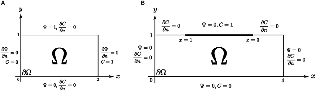
Figure 2. (A) Henry problem boundary conditions. (B) Elder problem boundary conditions.

2.2. Elder problem

The computational domain of the Elder problem is also a rectangular vertical cross-section that is filled with a homogeneous isotropic porous medium. Saltwater source is put along the middle of the top boundary. The bottom boundary is set at zero concentration. Governing equations for the Elder problem in dimensionless form can be expressed as in [5]:

$\begin{array}{lll}\frac{{\partial }^2\text{Ψ}}{\partial x^2}+\frac{{\partial }^2\text{Ψ}}{\partial y^2}& =Ra\frac{\partial C}{\partial x}& (3)\end{array}$

$\begin{array}{lll}\frac{{\partial }^{2}C}{\partial x^2}+\frac{{\partial }^{2}C}{\partial y^2}-\left(\frac{\partial \text{Ψ}}{\partial y}\frac{\partial C}{\partial x}-\frac{\partial \text{Ψ}}{\partial x}\frac{\partial C}{\partial y}\right)& =\frac{\partial C}{\partial t}& (4)\end{array}$

where Ra is the Rayleigh number which is a dimensionless parameter. Initial conditions are the same as in Henry problem, namely Ψ(x, y, 0) = 0 and C(x, y, 0) = 0. Boundary conditions for the stream function are zero on the four sides, which represents the fact that the velocity of the flow is zero along the boundary, and for that reason, there is no inflow on the boundaries. Further information for all boundary conditions is shown in the diagram in Figure 2B.

3. Proposed generalized finite difference scheme

The basic idea of the proposed generalized finite difference scheme, arises from considering the general second-order linear operator

$Lu=\lambda u_{xx}+\mu u_{xy}+\nu u_{yy}+\kappa u_x+\rho u_y+\sigma u$

where λ, μ, ν, κ, ρ, and σ are given functions of the spatial coordinates.

For an arbitrary star or distribution of nodes, for example, the one shown in Figure 3, the operator value at a central node p₀ = (x₀, y₀) could be approximated by using values of u at some neighbor nodes p_i = (x_i, y_i), i = 1, 2, …, q.

FIGURE 3

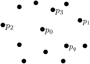
Figure 3. Arbitrary distribution of nodes.

A finite-difference scheme applied in p₀, can be seen as a linear combination

$L_{0}u={\Gamma }_{0}u(p_0)+{\Gamma }_{1}u(p_1)+\cdots +{\Gamma }_{q}u(p_q)={\displaystyle \sum _{i=0}^q}{\Gamma }_{i}u(p_i),$

where Γ₀, Γ₁, … , Γ_q are appropriate weights.

According to [12, 13], in order for a finite difference scheme, L₀, to be consistent with the linear operator L, it is required that the local truncation error τ satisfy

$\begin{array}{ll}\tau ={\left[Lu\right]}_{p_0}-{\left[L_{0}u\right]}_{p_0}\to 0& (5)\end{array}$

as p₁, p₂, … , p_q → p₀.

Expanding the consistency condition in the Taylor series,

$\begin{array}{l}{\left[Lu\right]}_{p_0}-{\left[L_{0}u\right]}_{p_0}\\ =\left(\sigma \left(p_0\right)-{\displaystyle \sum _{i=0}^q}{\Gamma }_i\right)u\left(p_0\right)+\left(\kappa \left(p_0\right)-{\displaystyle \sum _{i=1}^q}{\Gamma }_i\Delta x_i\right)u_x\left(p_0\right)\\ +\left(\rho \left(p_0\right)-{\displaystyle \sum _{i=1}^q}{\Gamma }_i\Delta y_i\right)u_y\left(p_0\right)+\left(\lambda \left(p_0\right)-{\displaystyle \sum _{i=1}^q}\frac{{\Gamma }_i{\left(\Delta x_i\right)}^2}{2}\right)u_{xx}\left(p_0\right)\\ +\left(\mu \left(p_0\right)-{\displaystyle \sum _{i=1}^q}{\Gamma }_i\Delta x_i\Delta y_i\right)u_{xy}\left(p_0\right)+\left(\nu \left(p_0\right)-{\displaystyle \sum _{i=1}^q}\frac{{\Gamma }_i{\left(\Delta y_i\right)}^2}{2}\right)\\ u_{yy}\left(p_0\right)+{O}{\left(max\left\{\Delta x_i,\Delta y_i\right\}\right)}^3\end{array}$

where Δx_i = x_i−x₀ and Δy_i = y_i−y₀.

To accomplish (5), each of the terms in brackets must vanish simultaneously; this is

$\begin{array}{l}\begin{array}{c}\lambda (p_0)-{\displaystyle \sum _{i=1}^q}\frac{{\Gamma }_i{(\Delta x_i)}^2}{2}=0,\\ \mu (p_0)-{\displaystyle \sum _{i=1}^q}{\Gamma }_i\Delta x_i\Delta y_i=0,\\ \nu (p_0)-{\displaystyle \sum _{i=1}^q}\frac{{\Gamma }_i{(\Delta y_i)}^2}{2}=0,\\ \end{array}\begin{array}{c}\kappa (p_0)-{\displaystyle \sum _{i=1}^q}{\Gamma }_i\Delta x_i=0,\\ \rho (p_0)-{\displaystyle \sum _{i=1}^q}{\Gamma }_i\Delta y_i=0,\\ \sigma (p_0)-{\displaystyle \sum _{i=0}^q}{\Gamma }_i=0.\\ \end{array}\end{array}$

This will define the linear system

$\begin{array}{ll}\left(\begin{array}{cccc}1& 1& \dots & 1\\ 0& \Delta x_1& \dots & \Delta x_q\\ 0& \Delta y_1& \dots & \Delta y_q\\ 0& {\left(\Delta x_1\right)}^2& \dots & {\left(\Delta x_q\right)}^2\\ 0& \Delta x_1\Delta y_1& \dots & \Delta x_q\Delta y_q\\ 0& {\left(\Delta y_1\right)}^2& \dots & {\left(\Delta y_q\right)}^2\\ \end{array}\right)\left(\begin{array}{c}{\Gamma }_0\\ {\Gamma }_1\\ {\Gamma }_2\\ .\hfill \\ .\hfill \\ .\hfill \\ {\Gamma }_q\\ \end{array}\right)=\left(\begin{array}{c}\sigma \left(p_0\right)\\ \kappa \left(p_0\right)\\ \rho \left(p_0\right)\\ 2\lambda \left(p_0\right)\\ \mu \left(p_0\right)\\ 2\nu \left(p_0\right)\\ \end{array}\right)& (6)\end{array}$

In order to solve this linear system, it is possible to separate the first equation of the system (6)

$\begin{array}{ll}{\displaystyle \sum _{i=0}^q}{\Gamma }_i-\sigma (p_0)=0& (7)\end{array}$

and then, the problem defined by

$\begin{array}{ll}\left(\begin{array}{lll}\Delta x_1& ...& \Delta x_q\\ \Delta y_1& ...& \Delta y_q\\ {\left(\Delta x_1\right)}^2& ...& {\left(\Delta x_q\right)}^2\\ \Delta x_1\Delta y_1& ...& \Delta x_q\Delta y_q\\ {\left(\Delta y_1\right)}^2& ...& {\left(\Delta y_q\right)}^2\\ \end{array}\right)\left(\begin{array}{c}{\Gamma }_1\\ {\Gamma }_2\hfill \\ .\hfill \\ .\hfill \\ .\hfill \\ {\Gamma }_q\\ \end{array}\right)=\left(\begin{array}{c}\kappa \left(p_0\right)\\ \rho \left(p_0\right)\\ 2\lambda \left(p_0\right)\\ \mu \left(p_0\right)\\ 2\nu \left(p_0\right)\\ \end{array}\right),& (8)\end{array}$

can be solved using the reduced Cholesky factorization of the normal equation for the full row rank matrix M, as in [24],

$M^{T}M\Gamma =M^T\beta ,$

where

$M=\left(\begin{array}{ccc}\Delta x_1& ...& \Delta x_q\\ \Delta y_1& ...& \Delta y_q\\ {\left(\Delta x_1\right)}^2& ...& {\left(\Delta x_q\right)}^2\\ \Delta x_1\Delta y_1& ...& \Delta x_q\Delta y_q\\ {\left(\Delta y_1\right)}^2& ...& {\left(\Delta y_q\right)}^2\\ \end{array}\right),\Gamma =\left(\begin{array}{c}{\Gamma }_1\\ {\Gamma }_2\\ .\hfill \\ .\hfill \\ .\hfill \\ {\Gamma }_q\\ \end{array}\right),\beta =\left(\begin{array}{c}\kappa \left(p_0\right)\\ \rho \left(p_0\right)\\ 2\lambda \left(p_0\right)\\ \mu \left(p_0\right)\\ 2\nu \left(p_0\right)\\ \end{array}\right),$

which defines the solution of an unweighted least-squares problem. The remaining value Γ₀ is then obtained from (7). Now, the obtained set of values Γ defines the proposed generalized finite differences scheme.

Thus, the scheme defined by Equation (8) can be used to approximate the standard differential operators at p₀. For instance, the approximation to the Laplacian operator is obtained by setting λ = ν = 1 and μ = κ = ρ = 0, while the approximation to the partial derivatives concerning x and y follows from κ = 1 and ρ = 1 (setting all the other coefficients equal to zero), respectively.

4. Numerical results

In this section, we show the numerical results obtained for the two benchmark problems. The numerical procedure comprises four steps

1. The node clouds were generated by taking the nodes from an initial nonuniform rectangular grid, which was used as a background geometric reference to define the stars. An essential detail is the generation of the initial non-rectangular grids. Bearing in mind the grid refinement process for the Motz problem as discussed in [25], since the graph of the solution C(x) is monotonic in several specific zones along the x-axis, we propose a mapping ξ ↦ x = ξ^α such that the expression

$\begin{array}{ll}\frac{\partial C}{\partial \xi }=\frac{\partial C}{\partial x}\frac{\partial x}{\partial \xi }& (9)\end{array}$

is almost constant. In this paper, the α = 1.5 was considered. This is the key to defining non-symmetric stars, which is a useful resource for the treatment of convective terms.

An example of the clouds obtained for the Henry problem is observed in Figure 4, which shows a cloud with N = 41 × 21 = 861 nodes.

2. To define the scheme and weights to apply the GFDM in the test problems, we considered specific simple stars which were generated from the clouds according to the following rule: at every inner grid node, two extra neighbors along a diagonal of the initial background grid were added to define a six-node star (q = 6; see an example on Figure 5A).

FIGURE 4

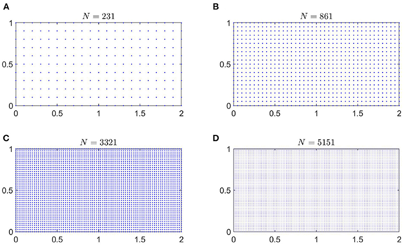
Figure 4. Clouds of nodes for the Henry problem, using different number of total nodes. (A) N = 21 × 11 = 231, (B) N = 41 × 21 = 861, (C) N = 81 × 41 = 3,321, and (D) N = 101 × 51 = 5,151.

The numerical treatment at the Neumann boundary condition

$\begin{array}{l}\frac{\partial u}{\partial n}(p_0)=l_x\frac{\partial u}{\partial x}+l_y\frac{\partial u}{\partial y}\end{array}$

where n = (l_x, l_y) is the outer normal vector at p₀, and is approximated using the scheme of Equation 8) with λ = μ = ρ = 0 and ν = l_x, κ = l_y using a star defined by six points: a ghost point p_g, the node p₀, and the five neighbors of the latter defined by the cells of the background grid for which p₀ was a corner (see Figure 5B), which yields the Equation (10)

$\begin{array}{ll}{l}_x\frac{\partial u}{\partial x}+l_y\frac{\partial u}{\partial y}\approx {\widehat{\Gamma }}_{g}u(p_g)+{\displaystyle \sum _{l=0}^5}{\widehat{\Gamma }}_{l}u(p_l),& (10)\end{array}$

or, in other words,

$\begin{array}{ll}u(p_g)=\frac{1}{{\widehat{\Gamma }}_g}\frac{\partial u}{\partial n}(p_0)-{\displaystyle \sum _{l=0}^5}\frac{{\widehat{\Gamma }}_l}{{\widehat{\Gamma }}_g}u(p_l).& (11)\end{array}$

For convenience, the ghost point p_g is calculated in such a way that p₀ is the midpoint of p_g and p_c, the latter being the neighbor in the negative direction of the outer normal vector −n. The value of u(p_g) given by the Equation (11) is substituted in the approximation to the governing equation at the boundary point p₀ using the same seven points p_g, p₀, and the five neighbors of the latter, which eliminates the value of u(p_g).

FIGURE 5

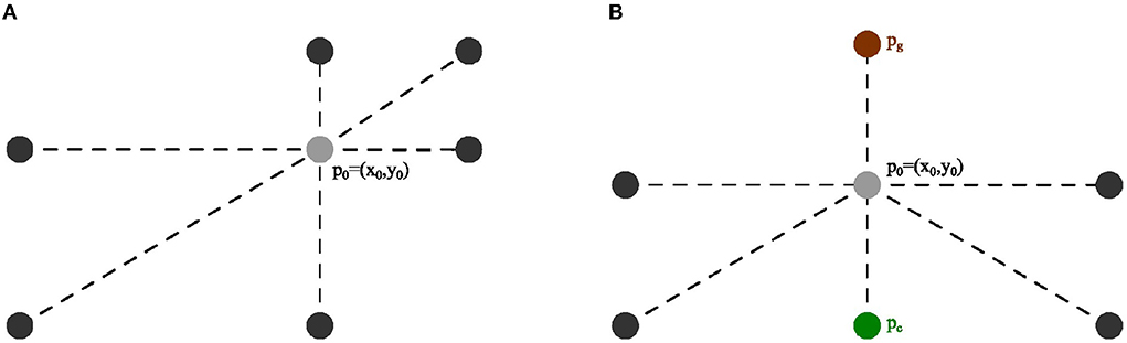
Figure 5. (A) Support nodes in the star at an inner node. (B) Support nodes in the star at a Neumann boundary node.

3. To produce the spatial discretization of the governing Equations (1) and (2), at every inner grid node the discretization given by Equation (8) was used with q = 6. The resulting governing equation after spatial discretization can be written in the form

$\begin{array}{lll}{D}_2\text{Ψ}-\frac{1}{a}{D}_{x}C& =0& (12)\end{array}$

$\begin{array}{lll}{D}_{2}C-\frac{1}{b}((D_y\text{Ψ}).*(D_{x}C)-(D_x\text{Ψ}).*(D_{y}C))& =\frac{\partial C}{\partial t}& (13)\end{array}$

where D₂ is a discrete Laplacian matrix, D_x is a differentiation matrix in the x direction, D_y is a differentiation matrix in the y direction. Ψ and C are column vectors of N rows that represent the unknown values of the stream function and the concentration at the cloud nodes. The product “.*” denotes element-wise multiplication. It must be noted that the differentiation matrices are very sparse because of the low number of star nodes.

Defining the vector U as

$\begin{array}{l}U=\left[\begin{array}{c}\text{Ψ}\\ C\end{array}\right]\end{array}$

and defining the matrix A and vector G as

$\begin{array}{r}A=\left(\begin{array}{cc}{D}_2& -\frac{1}{a}{D}_C\\ 0& D_2\end{array}\right),\\ G(U)=\left[\begin{array}{c}0\\ -\frac{1}{b}((D_y\text{Ψ}).*(D_{x}C)-(D_x\text{Ψ}).*(D_{y}C))\end{array}\right]\end{array}$

then Equations (12) and (13) can be written in the form

$\begin{array}{ll}\frac{dU}{dt}=AU+G(U)& (14)\end{array}$

where AU is the linear part of the problem, and G(U) is the non-linear part of the problem.

1. Finally, once the semi-discretized system (14) has been defined, for the time integration, a Runge-Kutta formula of the [26] family was used. The initial time step value was set to Δt = 0.01. At the nth step, the method attempts to calculate the next function value using the initial time step value. It calculates two approximations: one fourth-order and one fifth-order Runge-Kutta approximations. If the two approximations are sufficiently close, it accepts the fourth-order approximation and increases the step size slightly for the next step. If the two approximations disagree, It decreases Δt and tries again. At each step, it computes five values of the right-hand side of Equation (14) and combines them in two ways: one fourth-order and one fifth-order.

The results are compared against those obtained by other numerical methods and to those obtained using a semi-analytical solution.

4.1. Henry problem

Computational domain and boundary conditions for this problem can be observed in Figures 1, 2A, respectively. According to previous authors [5, 6, 10], there exist three versions of this problem. The first one is the original Henry problem, for which the constants are a = 0.2637 and b = 0.1. The second one is the Pinder version, where constant b is set as b = 0.035. And the third one is the modified Henry problem, where the constants have the values a = 0.1315 and b = 0.2. In this analysis, we examine the three versions of the Henry problem.

4.1.1. Original Henry problem (a = 0.2637, b = 0.1)

The first example is the original Henry saltwater intrusion problem (a = 0.2637, b = 0.1). Results for this problem (using different specific times) are shown in Figures 6, 7. Figure 6 shows the streamlines and Figure 7 displays concentration lines for different time values. Initially, the aquifer is filled with fresh water. The movement of the salt intrusion front in time can be observed in Figures 7A–E. The steady-state velocity vector field for this problem is plotted in Figure 8A. It is easy to see that a flow from left to right is due to the aquifer freshwater flow. There is an inflow on the right bottom domain caused by the saltwater intrusion from the sea. This produces a circulation that returns to the sea in the right top domain zone. For the concentration, it is apparent that there is a salt concentration moving into the domain because initially the aquifer is filled with fresh water. The steady-state results compare well with other solutions obtained with other methods, such as the network simulation method [5] and a different GFDM scheme [6]. To prove consistency in our method, a comparative plot was created using different number of total nodes (N = 21 × 11 = 231, N = 41 × 21 = 861, N = 81 × 41 = 3,321, and N = 101 × 51 = 5,151). Streamlines distribution and concentration distribution are observed in Figure 9, for different numbers of total nodes. In Figures 9B,D, corresponding to N = 231 and N = 861, respectively, it can be noticed that for the upper-right zone of the domain the concentration distribution presents difficulties. On the other hand (Figures 9F,H), corresponding to N = 231 and N = 861, respectively, show that when increasing the number of nodes N the concentration distribution becomes smoother at the conflicting upper-right zone of the domain.

FIGURE 6

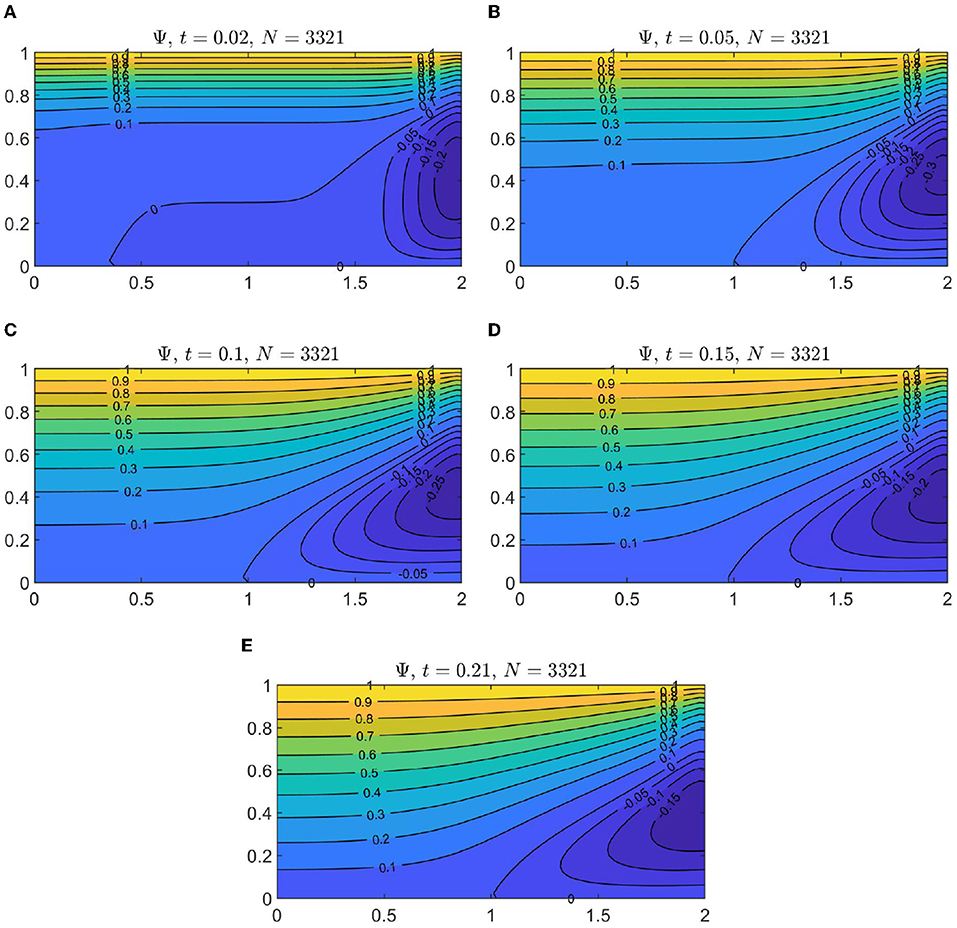
Figure 6. Streamlines distribution at different time for the original Henry problem. (A) t = 0.02, (B) t = 0.05, (C) t = 0.10, (D) t = 0.15, (E) steady-state t = 0.21 (a = 0.2637, b = 0.1, N = 81 × 41 = 3,321).

FIGURE 7

Figure 7. Concentration lines distribution at different time for the original Henry problem. (A) t = 0.02, (B) t = 0.05, (C) t = 0.10, (D) t = 0.15, (E) steady-state t = 0.21 (a = 0.2637, b = 0.1, N = 81 × 41 = 3,321).

FIGURE 8

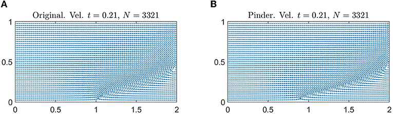
Figure 8. (A) Henry problem steady-state velocity vector field with normalized arrows (a = 0.2637, b = 0.1, N = 81 × 41 = 3,321). (B) Pinder version steady-state velocity vector field with normalized arrows (a = 0.2637, b = 0.035, N = 81 × 41 = 3,321).

FIGURE 9

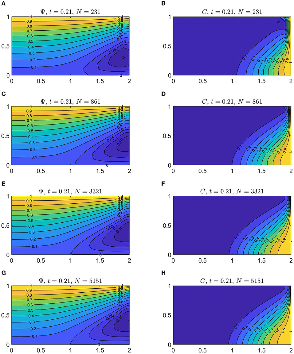
Figure 9. Steady-state streamlines distribution (Left) and steady-state concentration distribution (Right), for the Henry problem (a = 0.2637, b = 0.035) using different number of total nodes. (A,B) N = 21×11 = 231, (C,D) N = 41×21 = 861, (E,F) N = 81×41 = 3,321, (G,H) N = 101×51 = 5,151.

4.1.2. Pinder version of Henry problem (a = 0.2637, b = 0.035)

By comparison of the solutions obtained using a different number of total nodes, the consistency of the proposed scheme was validated. Now we use the same methodology to solve the Pinder version of Henry problem (a = 0.2637, b = 0.035), and test again consistency comparing solutions for this problem using different number of total nodes (N = 21 × 11 = 231, N = 41 × 21 = 861, N = 81 × 41 = 3,321, and N = 101 × 51 = 5,151). Figure 10 presents steady-state streamlines and concentration for a different number of total nodes. From Figures 9B,D, which correspond to steady-state solutions for the original Henry problem using a number of total nodes equal to 231 and 861, respectively, it can be observed that in the top right domain zone these solutions are different from those achieved using 3,321 and 5,151 number of total nodes (Figures 9F,H, respectively), but for the most part of the domain, these solutions can still be valid. An analogous argument can be made for describing (Figures 10B,D), which are steady-state solutions for the Pinder version of the Henry problem using 231 and 861 total nodes, respectively. As before, these solutions can still be valid for most parts of the domain. Figure 11A presents isochlor C = 0.5 for different number of total nodes (N = 21 × 11 = 231, N = 41 × 21 = 861, N = 81 × 41 = 3,321, and N = 101 × 51 = 5,151). It shows that solutions stably converge when the number of nodes increases.

FIGURE 10

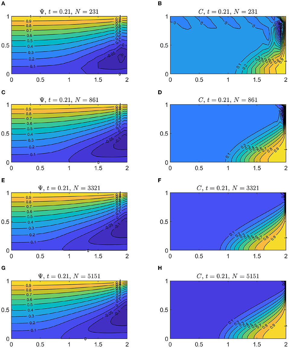
Figure 10. Steady-state streamline distributions (Left) and steady-state concentration distributions (Right), for Pinder version of Henry problem (a = 0.2637, b = 0.035) using different number of total nodes. (A,B) N = 21 × 11 = 231, (C,D) N = 41 × 21 = 861, (E,F) N = 81 × 41 = 3,321, (G,H) N = 101 × 51 = 5,151.

FIGURE 11

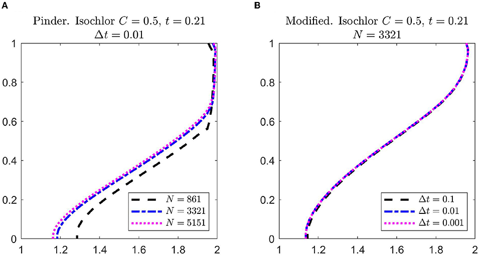
Figure 11. (A) Isochlor C = 0.5 for the Pinder version of Henry problem (a = 0.2637, b = 0.035), using different number of total nodes, N = 41 × 21 = 861, N = 81 × 41 = 3,321, and N = 101 × 51 = 5,151. (B) Isochlor C = 0.5 for the modified Henry problem (a = 0.1315, b = 0.2), using different time increments, Δt = 0.1, Δt = 0.01, Δt = 0.001.

Solutions obtained with 3,321 and 5,151 total nodes are like those obtained using other methods [5, 6]. Velocity vector field flow for the Pinder version is plotted in Figure 8B. Comparing steady-state concentration of the Pinder version and the original Henry problem, Figures 9H, 10H, respectively, it can be observed that the saltwater intrusion for the Pinder version is notably stronger than in the original Henry problem.

4.1.3. Modified Henry problem (a = 0.1315, b = 0.2)

For this problem steady-state streamlines distribution, concentration distribution, and velocity vector field are shown in Figure 12. Saltwater flux intrusion in the right bottom domain zone has increased, being the greatest of the three examples discussed.

FIGURE 12

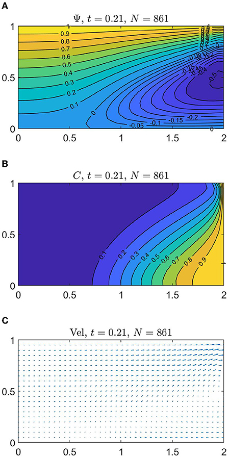
Figure 12. Modified Henry problem (a = 0.1315, b = 0.2). (A) Steady-state streamlines distribution. (B) Concentration distribution. (C) Velocity vector field.

In this example, we tested the method's stability by comparing solutions obtained using different time step sizes. Figure 11B shows isochlor C = 0.5 profiles of steady-state solutions with different time increments (Δt = 0.1, Δt = 0.01, and Δt = 0.001). The profiles are almost identical, proving the stability of the method.

Table 1 presents the xToe position of isochlor C = 0.5 using a different number of total nodes. The differences induced by parameters a and b in the different examples presented can be noticed, as well as the consistency of the method. Results in the presents study are comparable to the ones obtained using other methodologies [1–3, 5, 6, 10, 23, 27]; the results are compared in Table 2, which is updated from the table in [6]. However, some differences may be appreciated, which are caused by the selection of the support nodes for the approximation. In this paper, we chose six of the canonical support nodes (q = 6) shown in Figure 5A, and the regularity of the mesh makes the support nodes selection an automatic process. Thus, the problem is sparser and in consequence, the computational cost of the implementation is reduced. The stability, consistency, and simplicity of the method are validated by results obtained for the three versions of the Henry problem.

TABLE 1

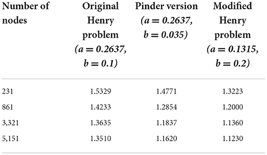
Table 1. Toe position for the isochlor C = 0.5, using different number of nodes.

TABLE 2

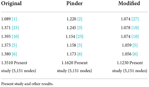
Table 2. Comparison of xToe position for the isochlor C = 0.5.

4.2. Elder problem

The second benchmark problem for groundwater flows is the Elder problem, which we analyze in this section. Parameters for this problem are Rayleigh number Ra = 400, a number of total nodes N = 121 × 56 = 6, 776, time step Δt = 0.001, and a number of support nodes (nodes in the star) q = 6 as in the previous section; in Figure 13 an example of the clouds used for the Elder problem can be observed. In this case figure shows a cloud of N = 41 × 11 = 451 nodes. Discretization for the spatial part of the Elder problem is very similar to that for the Henry problem of the preceding section, and the numerical treatment is the same. We can write discretized governing equations as

$\begin{array}{lll}{D}_2\text{Ψ}-Ra{D}_{x}C& =0& (15)\end{array}$

$\begin{array}{lll}{D}_{2}C-((D_y\text{Ψ}).*(D_{x}C)-(D_x\text{Ψ}).*(D_{y}C))& =\frac{\partial C}{\partial t}.& (16)\end{array}$

where D₂ is a discrete Laplacian matrix, D_x is a differentiation matrix in the x direction, D_y is a differentiation matrix in the y direction. Ψ and C are column vectors of N rows that represent the unknown values of the stream function and the concentration at the cloud nodes. The product “.*” denotes element-wise multiplication. As before it must be noted that the differentiation matrices are very sparse because of the low number of star nodes.

FIGURE 13

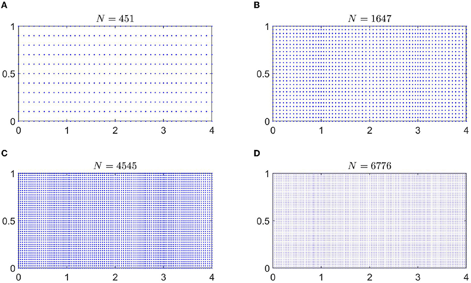
Figure 13. Clouds of nodes for the Elder problem, using different number of total nodes. (A) N = 41 × 11 = 451, (B) N = 61 × 27 = 1,647, (C) N = 101 × 45 = 4,545, and (D) N = 121 × 56 = 6, 776.

Defining the solution vector U, the matrix A, and the vector G as follows

$\begin{array}{r}U=\left[\begin{array}{c}\text{Ψ}\\ C\end{array}\right],A=\left(\begin{array}{cc}{D}_2& -Ra{D}_x\\ 0& D_2\end{array}\right),\\ G(U)=\left[\begin{array}{c}0\\ -((D_y\text{Ψ}).*(D_{x}C)-(D_x\text{Ψ}).*(D_{y}C))\end{array}\right]\end{array}$

then the Equations (15) and (16) can be written again in the form

$\begin{array}{ll}\frac{dU}{dt}=AU+G(U)& (17)\end{array}$

where, before, AU is the linear part of the problem, and G(U) is the non-linear part of the problem.

Boundary conditions are shown in Figure 2B and it can be observed that boundary conditions are symmetric to a vertical axis in x = 2. Because of symmetry, we show solutions only for the left half of the domain, from x = 0 to x = 2. We can observe steady-state streamlines distributions, concentration, and velocity vector field in Figure 14. From velocity (Figure 14C) three principal flow streams can be observed, although the salt concentration moves downwards (Figure 14B). This solution agrees with those obtained by [5, 6].

FIGURE 14

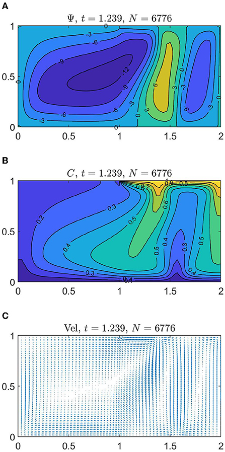
Figure 14. Steady-state solution to the Elder problem. (A) Streamlines distribution, (B) concentration distribution, (C) velocity vector field.

Figures 15, 16 show streamlines and concentration distributions for different time values (t = 0.005, t = 0.01, t = 0.02, t = 0.075, t = 0.1), and steady-state time t = 1.239 (see [6]). In order to prove consistency of the scheme proposed, results obtained for concentration at time t = 0.05, using different number of total nodes (N = 41 × 11 = 451, N = 61 × 27 = 1, 647, N = 101 × 45 = 4, 545, N = 121 × 56 = 6, 776) are shown in Figure 17 in which isochlors C = 0.2 and C = 0.6 are plotted for comparison.

FIGURE 15

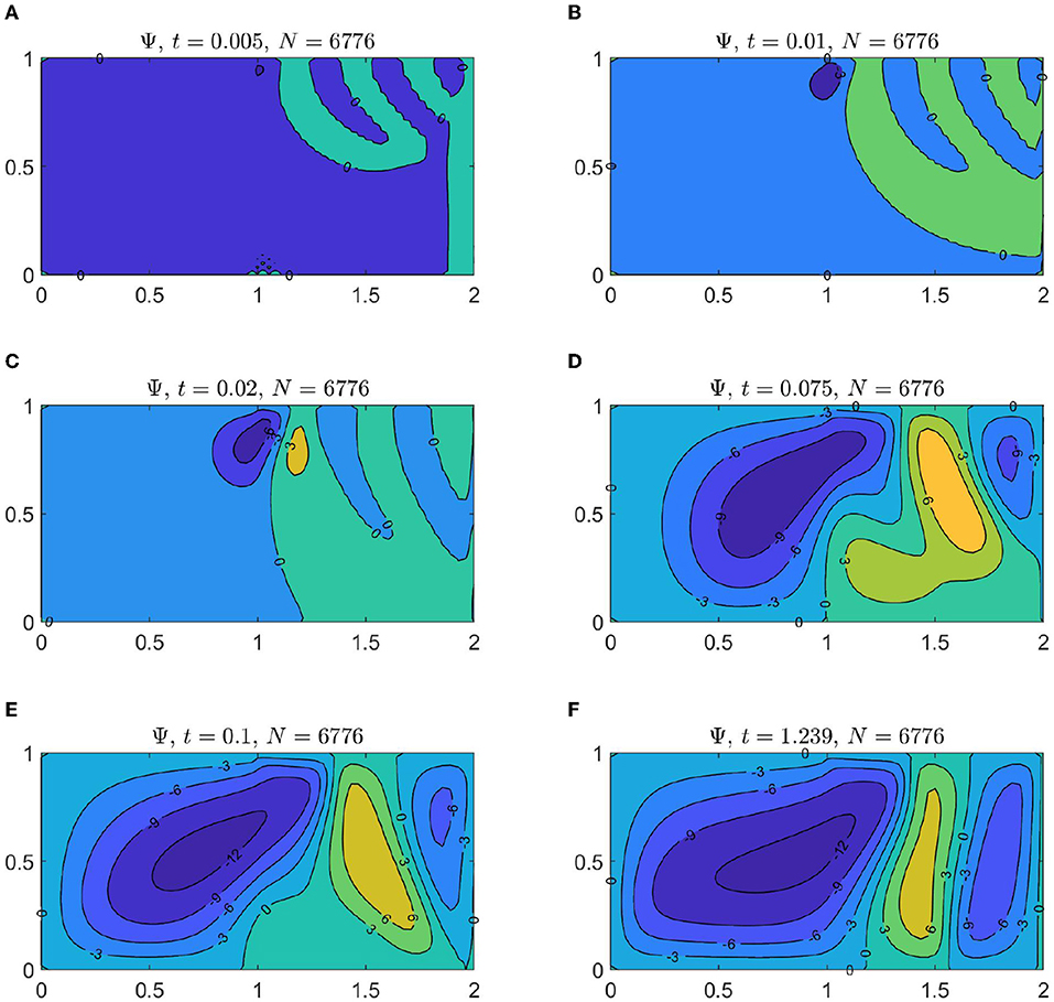
Figure 15. Streamlines distribution for different times. (A) t = 0.005, (B) t = 0.01, (C) t = 0.02, (D) t = 0.075, (E) t = 0.1, and (F) steady-state time t = 1.239.

FIGURE 16

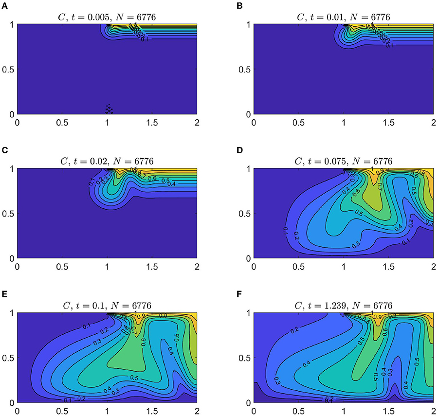
Figure 16. Concentration distribution for different times. (A) t = 0.005, (B) t = 0.01, (C) t = 0.02, (D) t = 0.075, (E) t = 0.1, and (F) steady-state time t = 1.239.

FIGURE 17

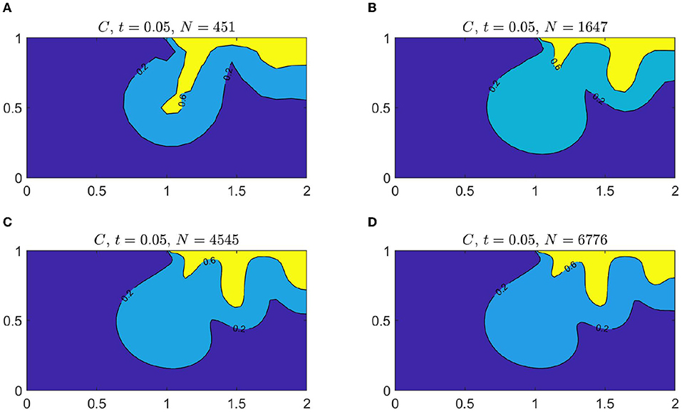
Figure 17. Isochlor C = 0.2 and C = 0.6 for different number of total nodes. (A) N = 41 × 11 = 451, (B) N = 61 × 27 = 1,647, (C) N = 101 × 45 = 4,545, and (D) N = 121 × 56 = 6,776.

5. Conclusions

In this paper, we presented a scheme of the generalized finite differences method (GFDM), which was useful for obtaining solutions for the Henry problem and the Elder problem, two benchmark problems concerning groundwater flows. We used both problems to test our version of the method's precision and stability by considering numerical experiments with three versions of the Henry problem: the original version, the Pinder version, and the modified version. To validate the proposed scheme, we tested with different numbers of total nodes N, and different time increments Δt. The main differences between our scheme and the proposed, among other authors, by [6, 28] are: First, We use only q = 6 support nodes while they made different tests using 12, 16, and 20 support nodes. In several papers, the number of support nodes is set to 27 for 2D problems. The use of a shorter number of support nodes as proposed in this paper makes the differentiation matrices to be sparser, although it must be acknowledged that problems with strong boundary layers or high gradient zones might require a larger number of support nodes in the stars. For instance, in [19], an effective star node selection for problems with strong convective terms is presented. In the end, the number of support nodes is problem dependent and requires further investigation. Second, because we generated the star nodes from initially structured clouds, the selection of support nodes is automatic and very simple, while in the aforementioned papers an additional algorithm for the selection of the support nodes had to be implemented. Certainly, very elaborated algorithms were discussed in them, but some problems like those presented here can be treated with very simple selection rules, although it is important to emphasize that, as mentioned in the preceding paragraph, other problems can require a stricter algorithm to define the stars. Third, and the final feature, in the proposed scheme, no weight function is required in the proposed GFDM. This is also a relevant difference concerning other variants of the method since, in consequence, the scheme is simpler, and the corresponding least square problem defined by Equation (8) is unweighted.

Thus, as the main conclusion, it is possible to assure that the proposed version of the GFDM is a useful numerical technique to solve the Elder problem and the Henry problem. It has the simplicity of the classical formulation of finite differences, but in addition, as has been discussed in other papers, it has the advantage that it can be applied even in non-structured clouds (see, for instance, [18, 29]), again, without requiring neither a weighting function nor a large number of support nodes as in some versions of the method.

In the end, the results of the numerical tests show that the GFDM is an interesting alternative numerical method to solve the Elder problem and the Henry problem. Bearing in mind the results of this paper and those of the references, this suggests that the GFDM is also an option for solving a wider range of differential equations.

Data availability statement

The original contributions presented in the study are included in the article/supplementary material, further inquiries can be directed to the corresponding author/s.

Author contributions

All authors listed have made a substantial, direct, and intellectual contribution to the work and approved it for publication.

Funding

Universidad Michoacana de San Nicolás de Hidalgo provides funds for open access publication fees, the International Centre for Numerical Methods in Engineering provides technical and academical support.

Acknowledgments

The authors wish to thank AULA CIMNE-Morelia and CIC-UMSNH for the support for this research. The authors would also like to thank the reviewers for their valuable feedback and suggestions to improve the present work.

Conflict of interest

The authors declare that the research was conducted in the absence of any commercial or financial relationships that could be construed as a potential conflict of interest.

Publisher's note

All claims expressed in this article are solely those of the authors and do not necessarily represent those of their affiliated organizations, or those of the publisher, the editors and the reviewers. Any product that may be evaluated in this article, or claim that may be made by its manufacturer, is not guaranteed or endorsed by the publisher.

References

1. Henry HR. Effects of dispersion on salt encroachment in coastal aquifers. In: Cooper Jr HH, Kohout FA, Henry HR, Glover RE, editors. Seawater in Coastal Aquifers. Washington, DC: US Geological Survey Water Supply Paper (1964). p. 70–80.

Google Scholar

2. Pinder GF, Cooper HH Jr. A numerical technique for calculating the transient position of the saltwater front. Water Resour Res. (1970) 6:875–82. doi: 10.1029/WR006i003p00875

CrossRef Full Text | Google Scholar

3. Segol G, Pinder GF, Gray WG. A Galerkin-finite element technique for calculating the transient position of the saltwater front. Water Resour Res. (1975) 11:343–7. doi: 10.1029/WR011i002p00343

CrossRef Full Text | Google Scholar

4. Simpson M, Clement T. Theoretical analysis of the worthiness of Henry and Elder problems as benchmarks of density-dependent groundwater flow models. Adv Water Resour. (2003) 26:17–31. doi: 10.1016/S0309-1708(02)00085-4

CrossRef Full Text | Google Scholar

5. Meca AS, Alhama F, Fernández CG. An efficient model for solving density driven groundwater flow problems based on the network simulation method. J Hydrol. (2007) 339:39–53. doi: 10.1016/j.jhydrol.2007.03.003

CrossRef Full Text | Google Scholar

6. Li PW, Fan CM, Chen CY, Ku CY. Generalized finite difference method for numerical solutions of density-driven groundwater flows. Comput Model Eng Sci. (2014) 101:319–50. doi: 10.3970/cmes.2014.101.319

CrossRef Full Text | Google Scholar

7. Fahs M, Ataie-Ashtiani B, Younes A, Simmons CT, Ackerer P. The Henry problem: New semianalytical solution for velocity-dependent dispersion. Water Resour Res. (2016) 52:7382–407. doi: 10.1002/2016WR019288

CrossRef Full Text | Google Scholar

8. Elder J. Transient convection in a porous medium. J Fluid Mech. (1967) 27:609–23. doi: 10.1017/S0022112067000576

CrossRef Full Text | Google Scholar

9. Zidane A, Younes A, Huggenberger P, Zechner E. The Henry semianalytical solution for saltwater intrusion with reduced dispersion. Water Resour Res. (2012) 48:1–10. doi: 10.1029/2011WR011157

CrossRef Full Text | Google Scholar

10. Simpson MJ, Clement TP. Improving the worthiness of the Henry problem as a benchmark for density-dependent groundwater flow models. Water Resour Res. (2004) 40:1–11. doi: 10.1029/2003WR002199

CrossRef Full Text | Google Scholar

11. Henry Saltwater Intrusion Problem (2015). Available online at: http://downloads.geo-slope.com/geostudioresources/7/examples/Henry%20Density%20Dependent.pdf

Google Scholar

12. Strikwerda JC. Finite Difference Schemes and Partial Differential Equations. Philadelphia, PA: SIAM (2004). doi: 10.1137/1.9780898717938

PubMed Abstract | CrossRef Full Text | Google Scholar

13. Thomas JW. Numerical Partial Differential Equations: Finite Difference Methods. Vol. 22. New York, NY: Springer Science & Business Media (2013).

PubMed Abstract | Google Scholar

14. Cortés-Medina A, Chávez-González A, Tinoco-Ruiz J. A direct finite-difference scheme for solving PDEs over general two-dimensional regions. Appl Numer Math. (2002) 40:219–33. doi: 10.1016/S0168-9274(01)00076-9

CrossRef Full Text | Google Scholar

15. Benito J, Urena F, Gavete L. Solving parabolic and hyperbolic equations by the generalized finite difference method. J Comput Appl Math. (2007) 209:208–33. doi: 10.1016/j.cam.2006.10.090

CrossRef Full Text | Google Scholar

16. Domínguez-Mota FJ, Armenta SM, Tinoco-Guerrero G, Tinoco-Ruiz JG. Finite difference schemes satisfying an optimality condition for the unsteady heat equation. Math Comput Simul. (2014) 106:76–83. doi: 10.1016/j.matcom.2014.02.007

CrossRef Full Text | Google Scholar

17. Prieto FU, Mu noz JJB, Corvinos LG. Application of the generalized finite difference method to solve the advection-diffusion equation. J Comput Appl Math. (2011) 235:1849–55. doi: 10.1016/j.cam.2010.05.026

CrossRef Full Text | Google Scholar

18. Chávez-Negrete C, Domínguez-Mota F, Santana-Quinteros D. Numerical solution of Richards' equation of water flow by generalized finite differences. Comput Geotechn. (2018) 101:168–75. doi: 10.1016/j.compgeo.2018.05.003

CrossRef Full Text | Google Scholar

19. Rao X, Liu Y, Zhao H. An upwind generalized finite difference method for meshless solution of two-phase porous flow equations. Eng Anal Bound Elements. (2022) 137:105–18. doi: 10.1016/j.enganabound.2022.01.013

CrossRef Full Text | Google Scholar

20. Rao X. An upwind generalized finite difference method (GFDM) for meshless analysis of heat and mass transfer in porous media. arXiv[Preprint].arXiv:211211005. (2021). doi: 10.48550/arXiv.2112.11005

CrossRef Full Text | Google Scholar

21. Rao X. A novel meshless method based on the virtual construction of node control domains for porous flow problems. arXiv[Preprint].arXiv:220605531. (2022). doi: 10.48550/arXiv.2206.05531

CrossRef Full Text | Google Scholar

22. Li PW, Chen W, Fu ZJ, Fan CM. Generalized finite difference method for solving the double-diffusive natural convection in fluid-saturated porous media. Eng Anal Bound Elem. (2018) 95:175–86. doi: 10.1016/j.enganabound.2018.06.014

CrossRef Full Text | Google Scholar

23. Gotovac H, Andricevic R, Gotovac B, Kozulic V, Vranjes M. An improved collocation method for solving the Henry problem. J Contam Hydrol. (2003) 64:129–49. doi: 10.1016/S0169-7722(02)00055-4

PubMed Abstract | CrossRef Full Text | Google Scholar

24. Tinoco-Guerrero G, Domínguez-Mota FJ, Tinoco-Ruiz JG. A study of the stability for a generalized finite-difference scheme applied to the advection-diffusion equation. Math Comput Simul. (2020) 176:301–11. doi: 10.1016/j.matcom.2020.01.020

CrossRef Full Text | Google Scholar

25. Chávez C, Mota FJD, Lucas-Martinez S, Tinoco-Ruiz JG, Quinteros DS. Generalized finite difference solution for the Motz Problem. Rev Int Métodos Numér Para Cálculo Dise Ingen. (2021) 37:1–7. doi: 10.23967/j.rimni.2021.01.004

CrossRef Full Text | Google Scholar

26. Dormand JR, Prince PJ. A family of embedded Runge-Kutta formulae. J Comput Appl Math. (1980) 6:19–26. doi: 10.1016/0771-050X(80)90013-3

CrossRef Full Text | Google Scholar

27. Langevin C, Guo W. Improvements to SEAWAT, a variable-density modeling code [abs.]. Eos Trans. (1999) 80:621–627.

Google Scholar

28. Benito J, Urena F, Gavete L. Influence of several factors in the generalized finite difference method. Appl Math Model. (2001) 25:1039–53. doi: 10.1016/S0307-904X(01)00029-4

PubMed Abstract | CrossRef Full Text | Google Scholar

29. Chávez-Negrete C, Santana-Quinteros D, Domínguez-Mota F. A solution of Richards' equation by generalized finite differences for stationary flow in a dam. Mathematics. (2021) 9:1604. doi: 10.3390/math9141604

CrossRef Full Text | Google Scholar