Wave solutions of the DMBBM equation and the cKG equation using the simple equation method

In this article, we transform the (1 + 1)-dimensional non-linear dispersive modified Benjamin-Bona-Mahony (DMBBM) equation and the (2 + 1)-dimensional cubic Klein Gordon (cKG) equation, which are the non-linear partial differential equations, into the non-linear ordinary differential equations by using the traveling wave transformation and solve these solutions with the simple equation method (SEM) with the Bernoulli equation. Two classes of exact explicit solutions-hyperbolic and trigonometric solutions of the associated NLEEs are characterized with some free parameters; we obtain the kink waves and periodic waves.

Introduction

Immediately, nonlinear evolution equations (NLEEs), i.e., partial differential equations with time derivatives and fractional differential equations (FDEs), have become a useful tool for describing the natural phenomena of science and engineering, such as optical fiber communications, atmospheric pollutant dispersion, solid state physics, signal processing, mechanical engineering, electric control theory, relativity, chemical reactions, etc. Exact solutions or numerical solutions have always played and still play an important role in properly understanding the qualitative features of many phenomena and processes in various fields of natural science. Various effective and powerful methods have been established to handle the NLEEs, such as the modified simple equation method [1, 2], the Jacobi elliptic function method [3], the (G′/G)-expansion method [4], the homotopy perturbation method [5], the variational iteration method [6], the Exp-function method [7, 8], the tanh function method [9], the F-expansion method [10], the Laplace-optimized decomposition method [11], the reproducing kernel algorithm [12–14] etc. The investigation of wave solutions of NLEEs plays a significant role in the study of nonlinear physical phenomena. The well-known wave solutions that are utilized to describe the exact solutions of NLEEs are lump solutions, lump-multi-kink solutions, and traveling wave solutions. Lump solutions and lump-multi-kink solutions to the (3 + 1) dimensional generalized Boiti–Leon–Manna–Pempinelli equation are studied in 2022 [15]. Lump-soliton solutions to the KPI equation are shown in 2021 [16]. Traveling wave solutions for the (2 + 1)-dimensional cubic nonlinear Klein–Gordon (cKG) equation and the (2 + 1)-dimensional nonlinear Zakharov–Kuznetsov modified equal width (ZK-MEW) equation were being investigated in 2019 [17]. Additionally, the (1 + 1)-dimensional nonlinear dispersive modified Benjamin-Bona Mahony (DMBBM) equation and the (2 + 1)-dimensional cubic Klein Gordon (cKG) equation are non-linear partial differential equations that play a significant role in various scientific and engineering fields. The DMBBM equation was first derived to describe an approximation for surface-long waves in non-linear dispersive media. It can also characterize the hydromagnetic waves in cold plasma, acoustic waves in inharmonic crystals, and acoustic gravity. The DMBBM was studied in 2010 using the extended (G′/G)-expansion method [18], and, in 2014, using the modified simple equation method [19]. The Klein-Gordon equation has been used to model a wide range of nonlinear phenomena, including the propagation of discrepancies in crystals and elementary particle behavior. This equation was studied in 2011 [20] using the extended (G′/G)-expansion method, in 2013 [21] using the modified simple equation method, and in 2019 [17] using the Riccati Bernoulli sub ODE method.

The simple equation method (SEM) was presented by Nikolai Kudryashov [22]. This method was created by two important ideas. One of them is to use the general solutions of the simplest non-linear differential equations. Another idea is to take into consideration all possible singularities in the equation studied. The simple equation method was used to investigate exact solutions of various equations, such as the Sharma Tasso Olver equation and the Burgers Huxley equation in 2008 [22], the Kodomtsev Petviashvili equation, the (2 + 1) dimensional breaking soliton equation, and the modified generalized Vakhnenko equation in 2016 [23] and the fourth-order non-linear AKNS water equation in 2021 [24].

In this article, we use the traveling wave to transform the DMBBM equation and the cKG equation into the nonlinear ordinary differential equations. Then, using the simple equation method with the Bernoulli equation, we obtain the precise solution of these equations in terms of the exponential functions, and the physical wave solution is created in the form of kink waves and periodic waves. Moreover, we compare these results presented with other results in order to show that the simple equation method with the Bernoulli equation is more convenient and easier to understand.

Algorithm of simple equation method

In this section, we present a direct method, namely, the simple equation method, for finding the traveling wave solution to nonlinear equations. Suppose that the nonlinear partial equation, in two independent variablesx and t, is given by:

$\begin{array}{ll}P(u,u_t,u_x,u_{tt},u_{xx},u_{xt},...)=0,& (1)\end{array}$

where u(x, t) is an unknown function, P is a polynomial of u(x, t) and its partial derivatives in which the highest-order derivatives and non–linear terms are involved. The main steps of the SE method [19] are as follows:

Step 1: Wave transformation

Combining the independent variables x and t into one variable ξ = x−ωt, we suppose that

$\begin{array}{ll}u(x,t)=u(\xi ),\xi =x-\omega t,& (2)\end{array}$

where ω is the speed of a traveling wave. The traveling wave transformation Equation (2) permits us to convert Equation (1) into an ordinary differential equation (ODE) for u = u(ξ):

$\begin{array}{ll}Q(u,u^{\prime },u^{″},...)=0,& (3)\end{array}$

where Q is a polynomial of u(ξ) and its derivatives in which the prime indicates the derivative with respect to ξ.

Step 2: Solution assumption

Assume that the formal solution of Equation (3) is of the form:

$\begin{array}{ll}u(\xi )={\displaystyle \sum _{i=0}^n}{a}_i{F}^i(\xi ),& (4)\end{array}$

where a_i(i = 0, 1, 2, ..., n) are constants that will be determined later and F(ξ) are the functions that satisfy the simple equations (ordinary differential equations). The simple equation has two characteristics. First of all, it lacks the order of Equation (2); secondly, we are aware of the general solution to the simple equation. In this article, we shall use the Bernoulli and Riccati equations, which are well-known nonlinear ordinary differential equations, and their solutions can be described by simple functions. Regarding the Bernoulli equation,

$\begin{array}{ll}{F}^{\prime }(\xi )=cF(\xi )+d{F}^2(\xi ).& (5)\end{array}$

Step 3: Finding the integer n

The positive integer n that occurs in Equation (4) can be estimated by taking into account the homogeneous balance between the highest-order derivative and the non-linear terms appearing in Equation (3).

Step 4: Solution attainment

We get the general solutions of the simple Equation (5) as follows:

Case I: if c > 0 and d < 0, we have

$\begin{array}{ll}F(\xi )=\frac{c{e}^{c(\xi +{\xi }_0)}}{1-d{e}^{c(\xi +{\xi }_0)}},& (6)\end{array}$

where ξ₀ is a constant of the integration.

Case II: if c < 0 and d > 0, we have

$\begin{array}{ll}F(\xi )=-\frac{c{e}^{c(\xi +{\xi }_0)}}{1+d{e}^{c(\xi +{\xi }_0)}},& (7)\end{array}$

where ξ₀ is a constant of the integration.

Application

In this section, we apply the proposed simple equation method to construct the traveling wave solution to solve the (1 + 1)-dimensional non-linear dispersive modified Benjamin-Bona-Mahony (DMBBM) and the (2 + 1)-dimensional cubic Klein Gordon equation.

Solution of the (1 + 1)-dimensional non-linear dispersive modified Benjamin-Bona- Mahony

The DMBBM equation is

$\begin{array}{ll}{u}_t+u_x-\alpha u^2{u}_x+u_{xxx}=0,& (8)\end{array}$

where α is a non-zero positive constant. Using the traveling wave variable ξ = x − ωt is transformed (8) into the following ODE:

$\begin{array}{ll}(1-\omega )u^{\prime }-\alpha u^2{u}^{\prime }+u^{‴}=0& (9)\end{array}$

According to the balancing procedure that will be described, the balancing number n is a positive integer, which can be defined by balancing the highest-order derivative terms with the highest power non-linear terms in Equation (9), i.e., n+3 = 3n+1, thus n = 1. We have the solution of Equation (9) as follows:

$\begin{array}{ll}u(\xi )={\displaystyle \sum _{i=0}^1}{a}_i{F}^i(\xi )=a_0+a_{1}F,& (10)\end{array}$

where F satisfies Equation (5); consequently, u′, u^‴ and u² can be expressed as follows:

$\begin{array}{r}{u}^{″}=a_1{c}^{2}F+3a_{1}cd{F}^2+2a_1{d}^2{F}^3,\\ u^{‴}=a_1{c}^{3}F+7a_1{c}^{2}d{F}^2+12a_{1}c{d}^2{F}^3+6a_1{d}^3{F}^4,\\ u^2=a_0^2+2a_0{a}_{1}F+a_1^2{F}^2.& (11)\end{array}$

Substituting Equations (10) and (11) into Equation (9) then equating the coefficient of F_i to zero, where i ≥ 0, yields

$\begin{array}{r}(1-\omega )a_{1}c-\alpha a_0^2{a}_{1}c+a_1{c}^3=0,\\ (1-\omega )a_{1}d-\alpha a_0^2{a}_{1}d-2\alpha a_0{a}_1^{2}c+7a_1{c}^{2}d=0,\\ -2\alpha a_0{a}_1^{2}d-\alpha a_1^{3}c+12a_{1}c{d}^2=0,\\ -\alpha a_1^{3}d+6a_1{d}^3=0.& (12)\end{array}$

Solving this system of algebraic equations, we obtain

$\begin{array}{ll}{a}_0=\frac{3c}{\sqrt{6\alpha }},a_1=d\sqrt{\frac{6}{\alpha }}and\omega =1-\frac{c^2}{2}.& (13)\end{array}$

or

$\begin{array}{ll}{a}_0=-\frac{3c}{\sqrt{6\alpha }},a_1=-d\sqrt{\frac{6}{\alpha }}and\omega =1-\frac{c^2}{2}.& (14)\end{array}$

Substituting Equations (13) and (14) into (10) yields the following two exact solutions. Then, we use the general solutions of Bernoulli equations (6) and (7). We get four exact solution (8) from the exponential term. Next, we set the constants c and d to obtain the exact solutions in hyperbolic form as follows:

Case I: if c = 1 and d = −1, we have

$\begin{array}{l}{u}_1\left(x,t\right)=-\frac{1}{2}\sqrt{\frac{6}{\alpha }}tanh\left(\frac{x-\frac{t}{2}+k}{2}\right),\\ u_2\left(x,t\right)=\frac{1}{2}\sqrt{\frac{6}{\alpha }}tanh\left(\frac{x-\frac{t}{2}+k}{2}\right).& (15)\end{array}$

Case II: if c = −1 and d = 1, we have

$\begin{array}{l}{u}_3\left(x,t\right)=\frac{1}{2}\sqrt{\frac{6}{\alpha }}tanh\left(\frac{-x+\frac{t}{2}+k}{2}\right),\\ u_4\left(x,t\right)=-\frac{1}{2}\sqrt{\frac{6}{\alpha }}tanh\left(\frac{-x+\frac{t}{2}+k}{2}\right),& (16)\end{array}$

where k is arbitrary constants, it might yield many new and more general exact solutions to the non-linear DMBBM equation.

Solution of the (2 + 1)-dimensional cubic Klein Gordon (cKG) equation

The (2 + 1)-dimensional cubic Klein Gordon (cKG) equation is

$\begin{array}{ll}{v}_{xx}+v_{yy}-v_{tt}+\alpha v+\beta v^3=0,& (17)\end{array}$

where α and β are non-zero positive constants. Using the traveling wave variable ξ = x + y − ωt is transformed (17) into the following ODE:

$\begin{array}{ll}(2-{\omega }^2)v^{″}+\alpha v+\beta v^3=0.& (18)\end{array}$

According to the balancing procedure that will be described, the balancing number n is a positive integer, which can be defined by balancing the highest-order derivative terms v″ with the highest power non-linear terms v³ in Equation (18), i.e., n + 2 = 3n; thus, n = 1. We have the solution of Equation (18) as follows:

$\begin{array}{ll}v(\xi )={\displaystyle \sum _{i=0}^1}{a}_i{F}^i(\xi )=a_0+a_{1}F,& (19)\end{array}$

where F satisfies Equation (5); consequently, and v³ can be expressed as follows:

$\begin{array}{r}{v}^{″}(\xi )=a_1{c}^{2}F+3a_{1}cd{F}^2+2a_1{d}^2{F}^3,\\ v^3(\xi )={a_0}^3+3{a_0}^2{a}_{1}F+3a_0{a_1}^2{F}^2+{a_1}^3{F}^3.& (20)\end{array}$

Substituting Equations (19) and (20) into Equation (18) and then equating the coefficient of F_i to zero, here i ≥ 0, yields

$\begin{array}{rr}\begin{array}{r}\alpha a_0+\beta {a_0}^3=0,\\ -({\omega }^2-2)a_1{c}^2+\alpha a_1+3\beta {a_0}^2{a}_1=0,\\ -3({\omega }^2-2)a_{1}cd+3\beta a_0{a_1}^2=0,\\ -2({\omega }^2-2)a_1{d}^2+\beta {a_1}^3=0.\end{array}& (21)\end{array}$

Solving this system of algebraic equations, we obtain

$\begin{array}{ll}{a}_0=i\sqrt{\frac{\alpha }{\beta }},a_1=d\sqrt{\frac{2({\omega }^2-2)}{\beta }}\text{ and }{\omega }^2-2=-\frac{2\alpha }{c^2}& (22)\end{array}$

or

$\begin{array}{r}{a}_0=-i\sqrt{\frac{\alpha }{\beta }},a_1=-d\sqrt{\frac{2({\omega }^2-2)}{\beta }}and{\omega }^2-2\\ =-\frac{2\alpha }{c^2}.& (23)\end{array}$

Substituting Equations (22) and (23) into (19) yields the following two exact solutions. Then, we use the general solutions of Bernoulli equations (6) and (7). We get four exact solutions of (17) from the exponential term. Next, we set the constants c and d to obtain the exact solutions in hyperbolic and trigonometric form as follows:

Case I: if d = −1 and c > 0, we have

$\begin{array}{ll}\begin{array}{c}{v}_1\left(x,y,t\right)=i\sqrt{\frac{\alpha }{\beta }}tanh\left(\frac{\sqrt{\frac{-2\alpha }{{\omega }^2-2}}\left(x+y-\omega t+k\right)}{2}\right),\\ v_2\left(x,y,t\right)=-i\sqrt{\frac{\alpha }{\beta }}tanh\left(\frac{\sqrt{\frac{-2\alpha }{{\omega }^2-2}}\left(x+y-\omega t+k\right)}{2}\right),\end{array}& (24)\end{array}$

where $c=\sqrt{\frac{-2\alpha }{{\omega }^2-2}}$ and k is arbitrary constants.

Case II: if and c < 0, we have

$\begin{array}{ll}\begin{array}{c}{v}_3\left(x,y,t\right)=\sqrt{\frac{\alpha }{\beta }}tan\left(\frac{\sqrt{\frac{2\alpha }{{\omega }^2-2}}\left(x+y-\omega t+k\right)}{2}\right),\\ v_4\left(x,y,t\right)=-\sqrt{\frac{\alpha }{\beta }}tan\left(\frac{\sqrt{\frac{2\alpha }{{\omega }^2-2}}\left(x+y-\omega t+k\right)}{2}\right),\end{array}& (25)\end{array}$

where $c=-\sqrt{\frac{-2\alpha }{{\omega }^2-2}}$ and k is arbitrary constants. It might yield many new and more general exact solutions to the non-linear cKG equation.

Graphical representation of some obtained solutions

In this section, we discuss the physical explanations and graphical representations of the solutions of the DMBBM equation and the cKG equation.

Graphical representation of the solution of the DMBBM equation

Upon utilizing the SE method, we achieve the traveling wave solutions of the DMBBM equation from Equations (15) and (16) when wave speed $\omega =1-\frac{c^2}{2}$. The solution u₁(x, t) represents by a singular kink-type wave for the parameter α = 6, k = 2 in the interval −10 ≤ x, t ≤ 10 and is shown in Figure 1 The kink wave rises or descends from one asymptotic state to another. The kink solution approaches a constant at infinity. The solutions u₂(x, t), u₃(x, t) and u₄(x, t) are analogous to the figures of solution u₁(x, t) and are presented in Figures 2–4, respectively.

FIGURE 1

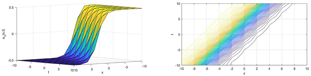
Figure 1. The kink wave solution of u₁(x, t) in 3D and contour.

FIGURE 2

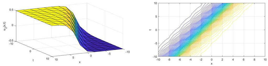
Figure 2. The kink wave solution of u₂(x, t) in 3D and contour.

FIGURE 3

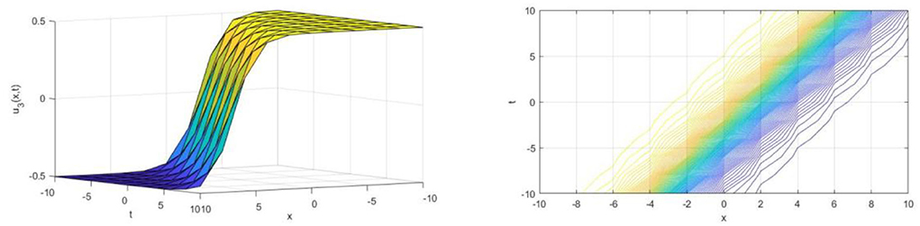
Figure 3. The kink wave solution of u₃(x, t) in 3D and contour.

FIGURE 4

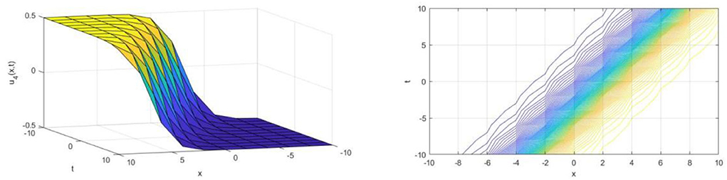
Figure 4. The kink wave solution of u₄(x, t) in 3D and contour.

Graphical representation of the cKG equation

In this subsection, we represent the shape of the solutions of the cKG equation in the form of Equations (24) and (25). The solution v₁(x, t) is formed by a singular kink-type wave when the wave speed ω = 2 and the parametersβ = 1, k = 2and α = −1 in the interval −10 ≤ x, t ≤ 10 and is demonstrated in Figure 5. This wave rises from one state to another state when t decreases. The solution v₂(x, t) also represents the same shape with v₁(x, t), but this wave raises from one state to another state when increased and is shown in Figure 6.

FIGURE 5

Figure 5. The kink wave solution of v₁(x, t) in 3D and contour.

FIGURE 6

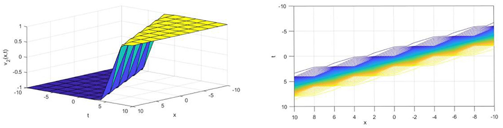
Figure 6. The kink wave solution of v₂(x, t) in 3D and contour.

The solutions v₃(x, t) and v₄(x, t) are a formed periodic traveling wave for the values β = 1, k = 2 and α = 1in the interval −10 ≤ x, t ≤ 10 and is presented in Figures 7, 8, respectively. A periodic traveling wave is a periodic function that moves with constant speed. Consequently, it is a special type of spatiotemporal oscillation that is a periodic function of both space and time.

FIGURE 7

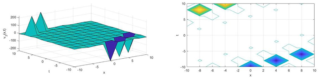
Figure 7. The periodic wave solution of in 3D and contour.

FIGURE 8

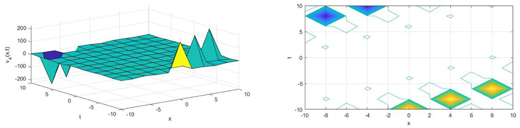
Figure 8. The periodic wave solution of in 3D and contour.

Comparisons

In this section, we compare our solutions with some well-known methods.

Comparisons of the solution of the DMBBM equation

In 2014, Khan et al. [19] investigated the exact solutions of the DMBBM equation by using the MSE method, and they got

$\begin{array}{l}{u}_{1,2}\left(x,t\right)=\pm \sqrt{\frac{3\left(1-\omega \right)}{\alpha }}tanh\left(\sqrt{\frac{1-\omega }{2}}\left(x-\omega t\right)\right)\end{array}$

and

$\begin{array}{l}{u}_{5,6}\left(x,t\right)=\pm \sqrt{\frac{3\left(\omega -1\right)}{\alpha }}tan\left(\sqrt{\frac{\omega -1}{2}}\left(x-\omega t\right)\right),\end{array}$

where c₁ = −2c₂(1−ω) are similar with our solutions, that is, c₁ = −1 and c₂ = 1, then u_{1, 2}(x, t) is identical with u₁(x, t) and u₂(x, t) where k = 0 and u_{5, 6}(x, t) are equal with u₃(x, t) and u₄(x, t) where k = 0.

Comparisons of the solution of the cKG equation

In 2019, Abdelrahman et al. [17] use the Riccati-Bernoulli sub-ODE method to investigate the exact solutions of the cKG equation.

$\begin{array}{l}{u}_{1,2}\left(x,t\right)=\pm \sqrt{\frac{\alpha }{\beta }}tan\left(\sqrt{\frac{\alpha }{2\left({\lambda }^2-2\right)}}\left(x+y-\lambda t+\mu \right)\right),\end{array}$

where $\frac{\alpha }{2({\lambda }^2-2)}>0$ is an identical with our solutions v₃(x, t) and v₄(x, t).

$\begin{array}{l}{u}_{5,6}\left(x,t\right)=\pm \sqrt{-\frac{\alpha }{\beta }}tanh\left(\sqrt{-\frac{\alpha }{2\left({\lambda }^2-2\right)}}\left(x+y-\lambda t+\mu \right)\right),\\ \end{array}$

where $\frac{\alpha }{2({\lambda }^2-2)}<0$ is an equal with our solutions v₁(x, t) and v₂(x, t).

The comparison of our exact solutions by using the SE method presented that the method is more convenient and the solutions have an easier format.

Conclusions

The simple equation method presented in this article has been successfully implemented to find the wave solutions for the DMBBM equation and the cKG equation. The method offers solutions with free parameters in the form of exponential, hyperbolic, and trigonometric functions that might be important to explain some intricate physical phenomena. Some special solutions, including the known traveling wave solution, are originated by setting appropriate values for the parameters. The wave effects of this equation were kink waves as shown in Figures 1–6 and periodic waves as displayed in Figures 7, 8. Compared to the currently proposed method with other methods, such as the MSE method and the Riccati-Bernoulli sub-ODE method, we assert that the SE method is a potent mathematical methodology, very simple, and has easy computations.

Data availability statement

The original contributions presented in the study are included in the article/supplementary material, further inquiries can be directed to the corresponding author.

Author contributions

All authors listed have made a substantial, direct, and intellectual contribution to the work and approved it for publication.

Conflict of interest

The authors declare that the research was conducted in the absence of any commercial or financial relationships that could be construed as a potential conflict of interest.

Publisher's note

All claims expressed in this article are solely those of the authors and do not necessarily represent those of their affiliated organizations, or those of the publisher, the editors and the reviewers. Any product that may be evaluated in this article, or claim that may be made by its manufacturer, is not guaranteed or endorsed by the publisher.

References

1. Akter J, Akbar MA. Exact solutions to the Benney-Luke equation and the Phi-4 equations by using modified simple equation method. Results Phys. (2015) 5. doi: 10.1016/j.rinp.2015.01.008

CrossRef Full Text | Google Scholar

2. Jawad AJM, Petkovic MD, Biswas A. Modified simple equation method for nonlinear evolution equations. Appl Math Comput. (2010) 217:2. doi: 10.1016/j.amc.2010.06.030

PubMed Abstract | CrossRef Full Text | Google Scholar

3. Ali AT. New generalized Jacobi elliptic function rational expansion method. J Comput Appl Math. (2011) 235:14. doi: 10.1016/j.cam.2011.03.002

CrossRef Full Text | Google Scholar

4. Akbar MA, Ali NHM, Roy R. Closed form solutions of two nonlinear time fractional wave equations. Results Phys. (2018) 9. doi: 10.1016/j.rinp.2018.03.059

CrossRef Full Text | Google Scholar

5. Roozi A, Alibeiki E, Hosseini SS, Shafiof SM, Ebrahimi M. Homotopy perturbation method for special nonlinear partial differential equations. J King Saud Univ (Sci). (2011) 23:1. doi: 10.1016/j.jksus.2010.06.014

CrossRef Full Text | Google Scholar

6. Abdou MA, Soliman AA. New applications of variational iteration method. Physical D: Nonlinear Phenomena. (2005) 211:1–2. doi: 10.1016/j.physd.2005.08.002

CrossRef Full Text | Google Scholar

7. He JH, Wu XH. Exp-function method for nonlinear wave equations. Chaos, Solitons Fractals. (2006) 30:3. doi: 10.1016/j.chaos.2006.03.020

PubMed Abstract | CrossRef Full Text | Google Scholar

8. Naher H, Abdullah AF, Akbar MA. New traveling wave solutions of the higher dimensional nonlinear partial differential equation by the Exp-function method. J Appl Math. (2012). doi: 10.1155/2012/575387

CrossRef Full Text | Google Scholar

9. Abdou MA. The extended tanh method and its applications for solving nonlinear physical models. Appl Math Comput. (2007) 190:1. doi: 10.1016/j.amc.2007.01.070

CrossRef Full Text | Google Scholar

10. Wang ML, Li XZ. Applications of F-expansion to periodic wave solutions for a new Hamiltonian amplitude equation. Chaos, Solitons Fractals. (2005) 24:5. doi: 10.1016/j.chaos.2004.09.044

CrossRef Full Text | Google Scholar

11. Beghami W, Maayah B, Bushnaq S, Abu Arqub O. The Laplace optimized decomposition method for solving systems of partial differential equations of fractional order. Int J App Computational Math. (2022) 8:52. doi: 10.1007/s40819-022-01256-x

CrossRef Full Text | Google Scholar

12. Djennadi S, Shawagfeh N, Abu Arqub O. A numerical algorithm in reproducing kernel-based approach for solving the inverse source problem of the time-space fractional diffusion equation. Partial Diff Equa Applied Math. (2021) 4. doi: 10.1016/j.padiff.2021.100164

CrossRef Full Text | Google Scholar

13. Momani S, Abu Arqub O, Maayah B. Piecewise optimal fractional reproducing kernel solution and convergence analysis for the Atangana–Baleanu–Caputo model of the Lienard's equation. Fractals. (2020)28:8. doi: 10.1142/S0218348X20400071

CrossRef Full Text | Google Scholar

14. Momani S, Maayah B, Abu Arqub O. The reproducing kernel algorithm for numerical solution of Van der Pol damping model in view of the Atangana–Baleanu fractional approach. Fractals. (2020) 28:08. doi: 10.1142/S0218348X20400101

CrossRef Full Text | Google Scholar

15. Chen SJ, Lü X. Lump and lump-multi-kink solutions in the (3+ 1)-dimensions. Commun Non-Linear Sci Num Simulation. (2022) 109. doi: 10.1016/j.cnsns.2021.106103

CrossRef Full Text | Google Scholar

16. Lü X, Chen SJ. New general interaction solutions to the KPI equation via an optional decoupling condition approach. Commun Non-Linear Sci Num Simulation. (2021) 103. doi: 10.1016/j.cnsns.2021.105939

CrossRef Full Text | Google Scholar

17. Abdelrahman MAE, Sohaly MA, Alharbi A. The new exact solutions for the deterministic and stochastic (2+1)-dimensional equations in natural sciences. J Taibah Univ Sci. (2019) 13:1. doi: 10.1080/16583655.2019.1644832

CrossRef Full Text | Google Scholar

18. Zayed EME, Joudi SA. Applications of an Extended (G'/G)-Expansion Method to Find Exact Solutions of Nonlinear PDEs in Mathematical Physics Mathematical Problems in Engineering. (2010). doi: 10.1155/2010/768573

CrossRef Full Text | Google Scholar

19. Khan K, Akbar MA, Islam SMR. Exact solutions for (1+1)-dimensional nonlinear dispersive modified Benjamin-Bona-Mahony equation and coupled Klein-Gordon equations. Springerplus. (2014) 3:1. doi: 10.1186/2193-1801-3-724

PubMed Abstract | CrossRef Full Text | Google Scholar

20. Zayed EME. The (G'/G)-expansion method combined with the Riccati equation for exact solutions of nonlinear PDES. Appl Math Informatics. (2011) 29:1–2.

Google Scholar

21. Khan K, Akbar MA. Exact solutions of the (2+1)-dimensional cubic Klein–Gordon equation and the (3+1) dimensional Zakharov Kuznetsov equation using the modified simple equation method. J Assoc Arab Univ Basic Appl Sci. (2013) 15. doi: 10.1016/j.jaubas.2013.05.001

CrossRef Full Text | Google Scholar

22. Kudryashov NA, Loguinova NB. Extended simplest equation method for nonlinear differential equations. Appl Math Comput. (2008) 205:1. doi: 10.1016/j.amc.2008.08.019

CrossRef Full Text | Google Scholar

23. Nofal TA. Simple equation method for nonlinear partial differential equations and its applications. J Egypt Math Soc. (2016) 24:2. doi: 10.1016/j.joems.2015.05.006

PubMed Abstract | CrossRef Full Text | Google Scholar

24. Phoosree S. New analytical solution of the fourth order nonlinear AKNS water equation. Proceedings of the 25 th Annual Meeting in Mathematics. (2021). p. 99–103.

Google Scholar