The Application of the Functional Variable Method for Solving the Loaded Non-linear Evaluation Equations

In this article, we construct exact traveling wave solutions of the loaded Korteweg-de Vries, the loaded modified Korteweg-de Vries, and the loaded Gardner equation by the functional variable method. The performance of this method is reliable and effective and gives the exact solitary and periodic wave solutions. All solutions to these equations have been examined and 3D graphics of the obtained solutions have been drawn by using the Matlab program. We get some traveling wave solutions, which are expressed by the hyperbolic functions and trigonometric functions. The graphical representations of some obtained solutions are demonstrated to better understand their physical features, including bell-shaped solitary wave solutions, singular soliton solutions, and solitary wave solutions of kink type. Our results reveal that the method is a very effective and straightforward way of formulating the exact traveling wave solutions of non-linear wave equations arising in mathematical physics and engineering.

1. Introduction

The investigation of exact traveling wave solutions to non-linear evolutions equations plays an important role in the study of non-linear physical phenomena. These equations arise in several fields of science, such as fluid dynamics, physics of plasmas, biological models, non-linear optics, chemical kinetics, quantum mechanics, ecological systems, electricity, ocean, and sea. One of the most important non-linear evolution equations is Korteweg De Vries (KdV) equation.

The KdV equation was first observed by John Scott Russell in experiments, and then Lord Rayleigh and Joseph Boussinesq studied it theoretically. Finally, in 1895, Korteweg and De Vries formulated a model equation to describe the aforementioned water wave, which helped to prove the existence of solitary waves. In the mid-1960s, Zabusky and Kruskal discovered the remarkably stable particle-like behavior of solitary waves. According to their study, solitary waves described by the KdV equation can pass through each other keeping their speed and shape unchanged. As a result, the name “soliton” is defined. In the wake of these discoveries, solitary wave theory boosted the development of many areas of science and technology. After 100 years, integrable systems developed deeply and soliton theory was widely applied in many areas. The KdV equation

$\begin{array}{ll}{u}_t+6u{u}_x+u_{xxx}=0,& (1)\end{array}$

has many connections to several branches of physics. The Equation (1) is especially important due to the potential application of different properties of electrostatic waves in the development of new theories of chemical physics, space environments, plasma physics, fluid dynamics, astrophysics, optical physics, nuclear physics, geophysics, dusty plasma, fluid mechanics, and different other fields of applied physics [1–11].

In recent years, studying electrostatic waves specifically to discuss different properties of solitary waves in the field of soliton dynamics has played a significant role for many researchers and has received considerable attention from them. The ion-acoustic solitary wave is one of the fundamental non-linear wave phenomena appearing in plasma physics. In 1973, Hans Schamel studies a modified Korteweg-de Vries equation for ion-acoustic waves which is expressed in the following basic form

$\begin{array}{ll}{u}_t+6u^2{u}_x+u_{xxx}=0.& (2)\end{array}$

This equation has been applied widely, e.g., in the molecular chain model, the generalized elastic solid, and so on [12–14]. Non-linear interactions between low-hybrid waves and plasmas can be described well by using the mKdV equation [15].

In 1968, the Gardner equation is an integrable non-linear partial differential equation introduced by the mathematician Clifford Gardner to generalize the KdV equation and modified the KdV equation. This equation can be written in a normalized form as follows:

$\begin{array}{ll}{u}_t+2\alpha u{u}_x+3\beta u^2{u}_x+u_{xxx}=0.& (3)\end{array}$

If the coefficient β > 0, Equation (3) admits two families of solitons and oscillating wave packets (called breathers), whereas if β < 0, only one category of solitons exists [16]. The Gardner equation plays an important role in various branches of physics, such as plasma physics, fluid physics, and quantum field theory [17, 18]. It also describes a variety of wave phenomena in plasma and solid state physics [19, 20].

In arterial mechanics, a model is widely used in which the artery is considered as a thin-walled prestressed elastic tube with a variable radius (or with stenosis) and blood as an ideal fluid [21]. The governing equation that models weakly non-linear waves in such fluid-filled elastic tubes is the modified Korteweg–de Vries equation

$u_t-6u^2{u}_x+u_{xxx}-h(t)u_x=0,$

where t - is a scaled coordinate along the axis of the vessel after static deformation characterizing axisymmetric stenosis on the surface of the arterial wall. x - is a variable that depends on time and coordinates along the axis of the vessel. h(t)- is a form of stenosis and u(x, t) characterizes the average axial velocity of the fluid.

We suppose that a form of stenosis h(t) is proportional to u(0, t), and we consider the loaded KdV, the loaded modified KdV and the loaded Gardner equation

$\begin{array}{ll}{u}_t-6\alpha u{u}_x+u_{xxx}+\gamma (t)u(0,t)u_x=0,& (4)\end{array}$

$\begin{array}{ll}{u}_t-12\alpha u^2{u}_x+u_{xxx}+\gamma (t)u(0,t)u_x=0,& (5)\end{array}$

$\begin{array}{ll}{u}_t+2\alpha u{u}_x+3\beta u^2{u}_x+u_{xxx}+\gamma (t)u(0,t)u_x=0,& (6)\end{array}$

where u(x, t) is an unknown function, x ∈ R, t ≥ 0, α, and β are any constants, γ(t) is the given real continuous function.

Many powerful and direct methods have been developed to find special solutions of non-linear evolution equations such as, Weierstrass elliptic function method [22], Jacobi elliptic function expansion method [23], tanh-function method [24], inverse scattering transform method [25], Hirota method [26], Backlund transform method [27], exp-function method [28], truncated Painleve expansion method [29], extended tanh-method [30], and the homogeneous balance method [31] are used for searching the exact solutions.

We establish exact traveling wave solutions of the loaded KdV, the loaded modified KdV, and the loaded Gardner equation by the functional variable method. The performance of this method is reliable and effective and gives the exact solitary wave solutions and periodic wave solutions. The traveling wave solutions obtained via this method are expressed by hyperbolic functions and trigonometric functions. The graphical representations of some obtained solutions are demonstrated to better understand their physical features, including bell-shaped solitary wave solutions, singular soliton solutions, and solitary wave solutions of kink type. This method presents wider applicability for handling non-linear wave equations.

In the recent years, the study of the stability of traveling waves of periodic and soliton types associated with non-linear dispersive equations has increased significantly. A rich variety of new mathematical problems have emerged, as well as the physical importance related to them. This subject is often studied in relation to the natural symmetries associated with the model and by perturbations of symmetric classes, e.g., the class of periodic functions with the same minimal period as the underlying wave. In the case of shallow-water wave models, a formal stability theory of periodic and soliton traveling waves has started.

It is known that the loaded differential equations contain some traces of an unknown function. In [32–38], the term “loaded equation” was used for the first time, the most general definitions of the loaded differential equation were given, and also detailed classifications of the differential loaded equations, as well as their numerous applications, were presented. A complete description of solutions of the non-linear loaded equations and their applications can be found in articles [39–45].

2. Description of the Functional Variable Method

Consider non-linear evolution equations with independent variables x, y, and t is of the form

$\begin{array}{ll}F(u,u_x,u_y,u_t,u_{xx},u_{tt},u_{yy},u_{xy},u_{xt},u_{yt}...)=0,& (7)\end{array}$

where F is a polynomial in u = u(x, y, t) and its partial derivatives. In [46, 47], Zerarka and others have summarized the functional variable method in the following:

Step 1. We use the wave transformation

$\begin{array}{ll}\xi =px+qy-kt,& (8)\end{array}$

where p and q are constants, and k is the speed of the traveling wave.

Next, we can introduce the following transformation for a traveling wave solution of Equation (7)

$\begin{array}{ll}u(x,y,t)=u(\xi ),& (9)\end{array}$

and the chain

$\begin{array}{ll}\frac{\partial u}{\partial x}=p\frac{du}{d\xi },\frac{\partial u}{\partial y}=q\frac{du}{d\xi },\frac{\partial u}{\partial t}=-k\frac{du}{d\xi },...& (10)\end{array}$

Using Equations (9) and (10), the non-linear partial differential Equation (7) can be transformed into an ordinary differential equation of the form

$\begin{array}{ll}P(u,u^{\prime },u^{″},u^{‴},...)=0,& (11)\end{array}$

where P is a polynomial in u(ξ) and its total derivatives, $u^{\prime }=\frac{du}{d\xi }$.

Step 2. Then we make a transformation in which the unknown function u is considered a functional variable in the form

$\begin{array}{ll}{u}^{\prime }=F(u),& (12)\end{array}$

then, the solution can be found by the relation

$\begin{array}{l}{\displaystyle \int }\frac{du}{F(u)}=\xi +{\xi }_0,\end{array}$

here, ξ₀ is a constant of integration which is set equal to zero for convenience. Some successive differentiations of u in terms of F are given as

$\begin{array}{l}{u}^{″}=\frac{dF(u)}{du}\frac{du}{d\xi }=\frac{dF(u)}{du}F(u)=\frac{1}{2}\frac{d(F^2(u))}{du},\\ u^{‴}=\frac{1}{2}\frac{d^2(F^2(u))}{d{u}^2}\sqrt{F^2(u)},\\ u^{‴\prime }=\frac{1}{2}\left[\frac{d^3(F^2(u))}{d{u}^3}{F}^2(u)+\frac{d^2(F^2(u))}{d{u}^2}\frac{d(F^2(u))}{du}\right].& (13)\end{array}$

Step 3. The ordinary differential Equation (11) can be reduced in terms of u, F, and its derivatives upon using the expressions of Equation (13) into Equation (7) gives

$\begin{array}{ll}H(u,\frac{dF(u)}{du},\frac{d^{2}F(u)}{d{u}^2},\frac{d^{3}F(u)}{d{u}^3},...)=0.& (14)\end{array}$

The key idea of this particular form Equation (14) is of special interest because it admits analytical solutions for a large class of non-linear wave type equations. After integration, Equation (14) provides the expression of F and this, together with Equation (12), give appropriate solutions to the original problem.

3. Solutions of the Loaded KdV Equation

We will show how to find the exact solution of the loaded KdV by the functional variable method. Using the wave variable

$\begin{array}{l}u(x,t)=u(\xi ),\xi =px-kt,\end{array}$

that will convert Equation (4) to an ordinary differential equation

$\begin{array}{ll}-k{u}^{\prime }-6\alpha pu{u}^{\prime }+p^3{u}^{‴}+\gamma (t)pu(0,t)u^{\prime }=0.& (15)\end{array}$

Integrating once Equation (15) with respect to ξ, and put the constant of integration zero, we have

$\begin{array}{ll}{u}^{″}=\frac{1}{p^3}\left(3\alpha p{u}^2+\left(k-\gamma \left(t\right)pu\left(0,t\right)\right)u\right).& (16)\end{array}$

Following Equation (13), it is easy to deduce from Equation (16) an expression for the function F(u)

$\begin{array}{ll}\frac{1}{2}\frac{d\left(F^2\left(u\right)\right)}{du}=\frac{1}{p^3}\left(3\alpha p{u}^2+\left(k-\gamma \left(t\right)pu\left(0,t\right)\right)u\right).& (17)\end{array}$

Integrating Equation (17) and setting the constant of integration to zero yields

$\begin{array}{l}{F}^2(u)=\frac{1}{p^3}\left(2\alpha p{u}^3+\left(k-\gamma (t)pu(0,t)\right)u^2\right)\\ F(u)=u\sqrt{\frac{2\alpha }{p^2}}\sqrt{u-\frac{\gamma (t)pu(0,t)-k}{2\alpha p}}\\ F(u)=u\sqrt{\frac{2\alpha }{p^2}}\sqrt{u-\eta (t)},& (18)\end{array}$

where $\eta (t)=\frac{\gamma (t)pu(0,t)-k}{2\alpha p}$. From Equation (12) and Equation (18), we deduce that

$\begin{array}{ll}\frac{du}{u\sqrt{u-\eta (t)}}=\sqrt{\frac{2\alpha }{p^2}}d\xi .& (19)\end{array}$

After integrating Equation (19), with zero constant of integration, we have the following exact solution

$\begin{array}{ll}u(x,t)=\frac{\gamma (t)pu(0,t)-k}{2\alpha p}\frac{1}{{cos}^2\sqrt{\frac{\gamma (t)pu(0,t)-k}{4p^3}}\left(px-kt\right)}.& (20)\end{array}$

It is obvious that the function u(0, t) can be easily found based on expression (20).

We have several types of traveling wave solutions of the loaded KdV equation as follows:

1) When $\sqrt{\frac{\gamma (t)pu(0,t)-k}{4p^3}}>0$, we have the periodic wave solution

$\begin{array}{l}u(x,t)=\frac{\gamma (t)pu(0,t)-k}{2\alpha p}\frac{1}{{cos}^2\sqrt{\frac{\gamma (t)pu(0,t)-k}{4p^3}}\left(px-kt\right)}.\end{array}$

2) When $\sqrt{\frac{\gamma (t)pu(0,t)-k}{4p^3}}<0$, we have the solitary wave solution

$\begin{array}{l}u(x,t)=\frac{\gamma (t)pu(0,t)-k}{2\alpha p}\frac{1}{{cosh}^2\sqrt{\frac{\gamma (t)pu(0,t)-k}{4p^3}}\left(px-kt\right)}.\end{array}$

Now, by choosing free parameters, we will write the traveling wave solutions of the loaded KdV equation in the simple form which can be used for the graphical illustrations.

If k = −1, α = 0.5, p = 1 and γ(t) = t, then we have

$\begin{array}{ll}u(x,t)=\frac{tu(0,t)+1}{{cos}^2\sqrt{\frac{tu(0,t)+1}{4}}(x+t)},& (21)\end{array}$

It is obvious that the function u(0, t) can be easily found based on expression (21).

If k = 1, α = 0.5, p = −1, and γ(t) = −t, then we have

$\begin{array}{ll}u(x,t)=-\frac{tu(0,t)+1}{{cosh}^2\sqrt{\frac{tu(0,t)+1}{4}}(t-x)},& (22)\end{array}$

It is obvious that the function u(0, t) can be easily found based on expression (22).

4. Graphical Representation of the Loaded KdV Equation

We have presented some graphs of solitary and periodic waves constructed by taking suitable values of the involved unknown parameters to visualize the underlying mechanism of the original physical phenomena. Using mathematical software Matlab, 3D plots of the obtained solutions have been shown in Figures 1, 2. A soliton or solitary wave in the concept of mathematical physics is defined as a self-reinforcing wave package that retains its shape. It propagates at a constant amplitude and velocity. Solitons are solutions of a common class of non-linearly partially differential equations with weak linearity describing physical systems. The existence of periodic traveling waves usually depends on the parameter values in a mathematical equation. If there is a periodic traveling wave solution, then there is typically a family of such solutions, with different wave speeds. For partial differential equations, periodic traveling waves typically occur for a continuous range of wave speeds. The physical description of the 3D loaded KdV equation of the installed exact moving wave solutions is discussed in this section. In the physical definition section, 3D surface drawings, contour maps, and 2D drawings of the developed moving wave solutions of the latest 3D loaded KdV equations are discussed. The 3D line plot emphasizes the amount of variability over time or compares multiple wave elements. The wave points were sequentially designed using equal interval breaks and connected by a line to emphasize the relationship of the wave points. Three-dimensional elegance is used to give visual attention to the diagram. Two-dimensional line drawings are used to represent very high and low frequencies and amplitudes.

FIGURE 1

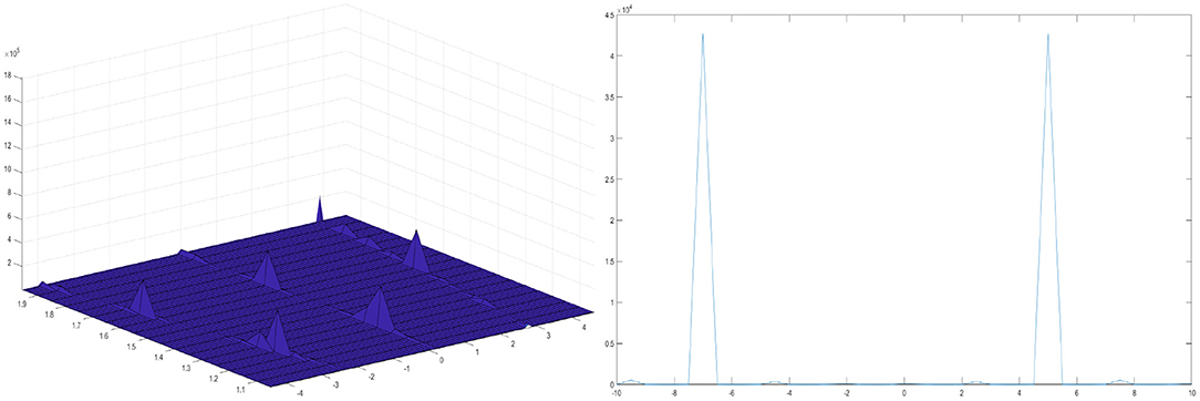
Figure 1. Periodic wave solution of the loaded KdV equation for k = −1, α = 0.5, p = 1, and γ(t) = t.

FIGURE 2

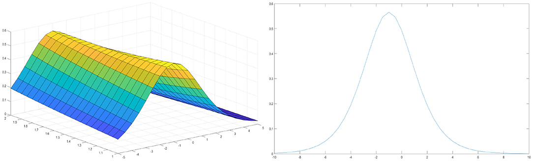
Figure 2. Solitary wave solution of the loaded KdV equation for k = 1, α = 0.5, p = −1, and γ(t) = −t.

5. Solutions of the Loaded Modified KdV Equation

Assume that Equation (5) has an exact solution in the form of a traveling wave

$\begin{array}{l}u(x,t)=u(\xi ),\xi =px-kt,\end{array}$

the Equation (5) can be converted to an ordinary differential equation

$\begin{array}{ll}-k{u}^{\prime }-12\alpha p{u}^2{u}^{\prime }+p^3{u}^{‴}+\gamma (t)pu(0,t)u^{\prime }=0.& (23)\end{array}$

Once integrating (23), setting the constant of integrating to zero, we obtain

$\begin{array}{ll}{u}^{″}=\frac{1}{p^3}\left(4\alpha p{u}^3+\left(k-\gamma (t)pu(0,t)\right)u\right).& (24)\end{array}$

Following Equation (13), it is easy to deduce from Equation (24) an expression for the function F(u)

$\begin{array}{ll}\frac{1}{2}\frac{d\left(F^2(u)\right)}{du}=\frac{1}{p^3}\left(4\alpha p{u}^3+\left(k-\gamma (t)pu(0,t)\right)u\right).& (25)\end{array}$

Integrating Equation (25) with respect to u and after the mathematical manipulations, we have

$\begin{array}{l}{F}^2(u)=\frac{1}{p^3}\left(2\alpha p{u}^4+\left(k-\gamma (t)pu(0,t)\right)u^2\right)\\ F(u)=\frac{u}{p}\sqrt{2\alpha }\sqrt{u^2-\frac{\gamma (t)pu(0,t)-k}{2\alpha p}}\\ F(u)=\frac{u}{p}\sqrt{2\alpha }\sqrt{u^2-\phi (t)},& (26)\end{array}$

where $\phi (t)=\frac{\gamma (t)pu(0,t)-k}{2\alpha p}$. From Equation (12) and Equation (26), we deduce that

$\begin{array}{ll}\frac{du}{u\sqrt{u^2-\phi (t)}}=\frac{\sqrt{2\alpha }}{p}d\xi .& (27)\end{array}$

After integrating Equation (27), with zero constant of integration, we have the following exact solution

$\begin{array}{ll}u(x,t)=\sqrt{\frac{\gamma (t)pu(0,t)-k}{2\alpha p}}\frac{1}{cos\sqrt{\frac{\gamma (t)pu(0,t)-k}{p^3}}\left(px-kt\right)}.& (28)\end{array}$

It is obvious that the function u(0, t) can be easily found based on expression (28).

We have several types of traveling wave solutions of the loaded modified KdV equation as follows:

1) When $\sqrt{\frac{\gamma (t)pu(0,t)-k}{p^3}}>0,\alpha >0$, we have the periodic wave solution

$\begin{array}{l}u(x,t)=\sqrt{\frac{\gamma (t)pu(0,t)-k}{2\alpha p}}\frac{1}{cos\sqrt{\frac{\gamma (t)pu(0,t)-k}{p^3}}\left(px-kt\right)}.\end{array}$

2) When $\sqrt{\frac{\gamma (t)pu(0,t)-k}{p^3}}<0,\alpha <0$, we have the solitary wave solution

$\begin{array}{l}u(x,t)=\sqrt{\frac{\gamma (t)pu(0,t)-k}{2\alpha p}}\frac{1}{cosh\sqrt{\frac{\gamma (t)pu(0,t)-k}{p^3}}\left(px-kt\right)}.\end{array}$

Now, by choosing free parameters, we will write the traveling wave solutions of the loaded modified KdV equation in the simple form which can be used for the graphical illustrations.

If k = −1, α = 0.5, p = 1, and γ(t) = t, then we have

$\begin{array}{ll}u(x,t)=\frac{\sqrt{tu(0,t)+1}}{cos\sqrt{tu(0,t)+1}(x+t)},& (29)\end{array}$

It is obvious that the function u(0, t) can be easily found based on expression (29).

If k = 1, α = −0.5, p = 1, and γ(t) = −t, then we have

$\begin{array}{ll}u(x,t)=\frac{\sqrt{tu(0,t)+1}}{cosh\sqrt{tu(0,t)-1}(x-t)},& (30)\end{array}$

It is obvious that the function u(0, t) can be easily found based on expression (30).

6. Physical Explanation of the Loaded Modified KdV Equation

We have shown how to find the solutions of the loaded modified KdV equation in 3D plot formats to make it easier to imagine. Graphical representation is an effective tool for communication and it exemplifies evidently the solutions to the problems. The graphical illustrations of the solutions are depicted in Figures 3, 4. Solitary and periodic wave solutions represent an important type of solutions for non-linear partial differential equations as many non-linear partial differential equations have been found to have a variety of solitary wave solutions. The solitary wave solutions obtained in this article are encouraging, applicable, and could be helpful in analyzing long wave propagation on the surface of a fluid layer under the action of gravity, iron sound waves in plasma, and vibrations in a non-linear string.

FIGURE 3

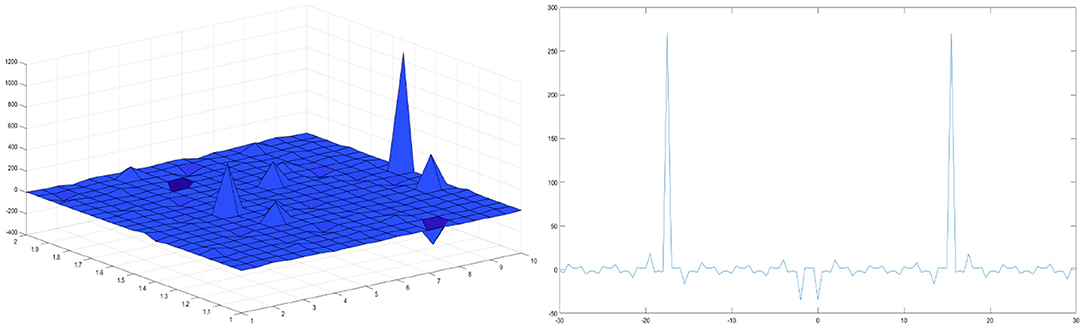
Figure 3. Periodic wave solution of the loaded modified KdV equation for k = −1, α = 0.5, p = 1, and γ(t) = t.

FIGURE 4

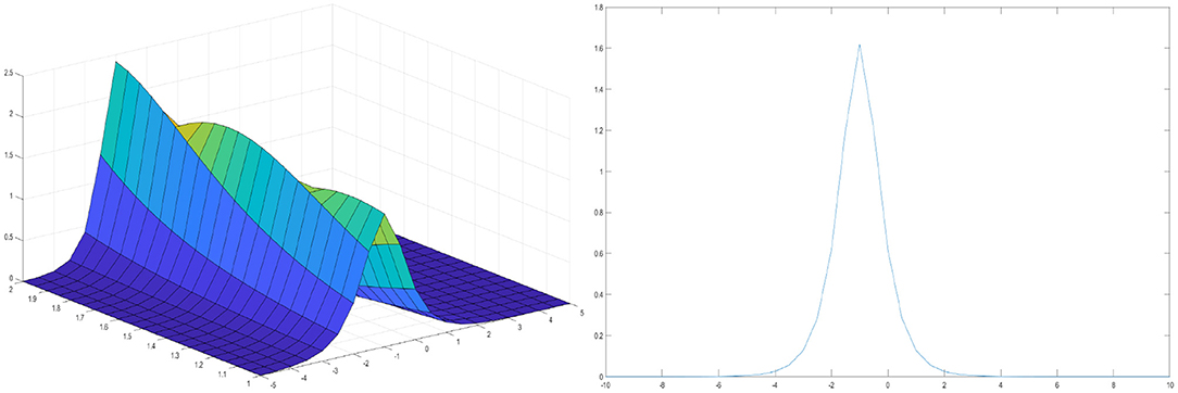
Figure 4. Solitary wave solution of the loaded modified KdV equation for k = 1, α = −0.5, p = 1, and γ(t) = −t.

7. Solutions of the Loaded Gardner Equation

Assume that Equation (6) has an exact solution in the form of a traveling wave

$\begin{array}{l}u(x,t)=u(\xi ),\xi =px-kt,\end{array}$

that will convert Equation (6) to an ordinary differential equation

$\begin{array}{ll}-k{u}^{\prime }-2\alpha pu{u}^{\prime }-3\beta u^2{u}^{\prime }+p^3{u}^{‴}+\gamma (t)pu(0,t)u^{\prime }=0.& (31)\end{array}$

Integrating once Equation (31) with respect to ξ, and putting the constant of integration at zero, we have

$\begin{array}{ll}{u}^{″}=\frac{1}{p^3}\left(\beta u^3+\alpha p{u}^2+\left(k-\gamma \left(t\right)pu\left(0,t\right)\right)u\right).& (32)\end{array}$

Following Equation (13), it is easy to deduce from Equation (32) an expression for the function F(u)

$\begin{array}{ll}\frac{1}{2}\frac{d(F^2(u))}{du}=\frac{1}{p^3}(\beta u^3+\alpha p{u}^2+(k-\gamma (t)pu(0,t))u).& (33)\end{array}$

Integrating Equation (33) and setting the constant of integration to zero yields

$\begin{array}{ll}F(u)=\frac{u}{p}\sqrt{\lambda u^2+\tau u+\mu (t)},& (34)\end{array}$

where $\lambda =\frac{\beta }{2p},\tau =\frac{2\alpha }{3},\mu (t)=\frac{k-\gamma (t)pu(0,t)}{p}$. From Equation (12) and Equation (34), we deduce that

$\begin{array}{ll}\frac{du}{u\sqrt{\lambda u^2+\tau u+\mu (t)}}=\frac{1}{p}d\xi .& (35)\end{array}$

After integrating Equation (35), with zero constant of integration, we have the following exact solution

$\begin{array}{ll}u(x,t)=\frac{2\mu (t)e^{-\frac{\sqrt{\mu (t)}}{p}(px-kt)}}{{\left(e^{-\frac{\sqrt{\mu (t)}}{p}(px-kt)}-\frac{\tau }{2}\right)}^2-{\frac{\tau }{2}}^2-\lambda \mu (t)}.& (36)\end{array}$

It is obvious that the function u(0, t) can be easily found based on expression (36).

We have several types of traveling wave solutions of the loaded Gardner equation as follows:

1) When $\sqrt{\mu (t)}>0$, we have the periodic wave solution

$\begin{array}{l}u(x,t)=\frac{2\mu (t)e^{-\frac{\sqrt{\mu (t)}}{p}(px-kt)}}{{\left(e^{-\frac{\sqrt{\mu (t)}}{p}(px-kt)}-\frac{\tau }{2}\right)}^2-{\frac{\tau }{2}}^2-\lambda \mu (t)}.\end{array}$

2) When $\sqrt{\mu (t)}<0$, we have the solitary wave solution

$\begin{array}{l}u(x,t)=\frac{2\mu (t)e^{-\frac{\sqrt{\mu (t)}}{p}(px-kt)i}}{{\left(e^{-\frac{\sqrt{\mu (t)}}{p}(px-kt)i}-\frac{\tau }{2}\right)}^2-{\frac{\tau }{2}}^2-\lambda \mu (t)}.\end{array}$

Now, by choosing free parameters, we will write the traveling wave solutions of the loaded Gardner equation in the simple form which can be used for the graphical illustrations.

If k = 1, α = 3, p = −1, β = 2, γ(t) = −t, then we have

$\begin{array}{ll}u(x,t)=\frac{2\left(tu(0,t)-1\right)e^{\sqrt{tu(0,t)-1}(x+t)}}{{\left(e^{\sqrt{tu(0,t)-1}(x+t)}-1\right)}^2+tu(0,t)-1},& (37)\end{array}$

It is obvious that the function u(0, t) can be easily found based on expression (37).

If k = 1, α = 3, p = −1, β = 2, γ(t) = t, then we have

$\begin{array}{ll}u(x,t)=-\frac{2(tu(0,t)+1)e^{\sqrt{tpu(0,t)+1}(x+t)i}}{{\left(e^{\sqrt{tpu(0,t)+1}(x+t)i}-1\right)}^2-\left(tu(0,t)+1\right)},& (38)\end{array}$

It is obvious that the function u(0, t) can be easily found based on expression (38).

8. Graphical Representations of Traveling Wave Solutions of the Loaded Gardner Equation

This section aims to present graphical illustrations of the obtained traveling wave solutions of the Gardner equation. Using mathematical software Matlab, 3D plots of the obtained solutions have been shown in Figures 5, 6. In the concept of mathematical physics, a soliton or solitary wave is defined as a self-reinforcing wave packet that upholds its shape. At the same time, it propagates at a constant amplitude and velocity. Solitary waves can be obtained from each traveling wave solution by setting particular values to its unknown parameters. By adjusting these parameters, one can get an internal localized mode. We have presented some graphs of solitary waves constructed by taking suitable values of the involved unknown parameters to visualize the underlying mechanism of the original physical phenomena.

FIGURE 5

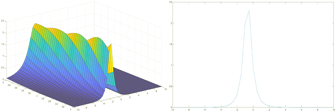
Figure 5. Solitary wave solution of the loaded Gardner equation for k = 1, α = 3, p = −1, β = 2, γ(t) = −t.

FIGURE 6

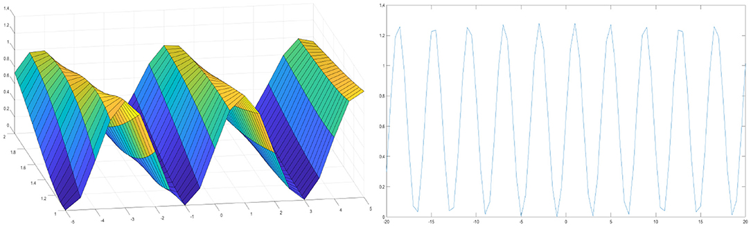
Figure 6. Periodic wave solution of the loaded Gardner equation for k = 1, α = 3, p = −1, β = 2, γ(t) = t.

9. Conclusion

The functional variable method has been successfully used to obtain several traveling wave solutions of the loaded KdV, the loaded modified KdV, and the loaded Gardner equation. The method does not require linearization of differential equations because it is a method of directly solving some non-linear physical models. A wide and general class of modern examples representing real physical problems from plasma physics, fluid dynamics, non-linear optics, and non-linear fields of gas dynamics can be solved easily and elegantly using this method. The exactness of the obtained results is studied by using the software Matlab. The received solutions with free parameters may be important to explain some physical phenomena. The advantage of the method is to give more solution functions such as periodic solutions and hyperbolic solutions than other popular analytical methods. We conclude that the functional variable method is significant and important for finding the exact traveling wave solutions of non-linear evolution equations. The proposed method can be applied to many other non-linear evolution equations in mathematical physics.

Data Availability Statement

The original contributions presented in the study are included in the article/supplementary material, further inquiries can be directed to the corresponding author/s.

Author Contributions

BB and FA conceived of the presented idea. BB developed the theory and performed the computations. FA verified the analytical methods. Both authors discussed the results and contributed to the final manuscript. Both authors contributed to the article and approved the submitted version.

Conflict of Interest

The authors declare that the research was conducted in the absence of any commercial or financial relationships that could be construed as a potential conflict of interest.

Publisher's Note

All claims expressed in this article are solely those of the authors and do not necessarily represent those of their affiliated organizations, or those of the publisher, the editors and the reviewers. Any product that may be evaluated in this article, or claim that may be made by its manufacturer, is not guaranteed or endorsed by the publisher.

References

1. Sagdeev RZ. Cooperative phenomena and shock waves in collision less plasmas. Rev Plasma Phys. (1966) 4:23–91.

Google Scholar

2. Seadawy AR, Nadia C. Some new families of spiky solitary waves of one-dimensional higher-order KdV equation with power law nonlinearity in plasma physics. Indian J Phys. (2020) 94:117–26. doi: 10.1007/s12648-019-01442-6

CrossRef Full Text | Google Scholar

3. Seadawy AR, Nadia C. Propagation of nonlinear complex waves for the coupled nonlinear Schrödinger Equations in two core optical fibers. Phys A Stat Mech Appl. (2019) 529:13–30. doi: 10.1016/j.physa.2019.121330

CrossRef Full Text | Google Scholar

4. Seadawy AR, Nadia C. Applications of extended modified auxiliary equation mapping method for high order dispersive extended nonlinear Schrödinger equation in nonlinear. Modern Phys Lett B. (2019) 33:1–11. doi: 10.1142/S0217984919502038

CrossRef Full Text | Google Scholar

5. Nadia C, Seadawy AR, Sheng C. More general families of exact solitary wave solutions of the nonlinear Schrödinger equation with their applications in nonlinear optics. Eur Phys J Plus. (2018) 133:547. doi: 10.1140/epjp/i2018-12354-9

CrossRef Full Text | Google Scholar

6. Tagare SG, Singh SV, Reddy RV, Lakhina GS. Electron-acoustic solitons in the Earth's magnetotail. Nonlinear Process Geophys. (2004) 11:215–8. doi: 10.5194/npg-11-215-2004

CrossRef Full Text | Google Scholar

7. Kakad AP, Singh SV, Reddy RV, Lakhina GS, Tagare SG. Electron acoustic solitary waves in the earth's magnetotail region. Adv Space Res. (2009) 43:1945–9. doi: 10.1016/j.asr.2009.03.005

CrossRef Full Text | Google Scholar

8. Abu Arqub O, Rashaideh H. The RKHS method for numerical treatment for integrodifferential algebraic systems of temporal two-point BVPs. Neural Comput Appl. (2018) 30:2595–606. doi: 10.1007/s00521-017-2845-7

CrossRef Full Text | Google Scholar

9. Abu Arqub O. Computational algorithm for solving singular Fredholm time-fractional partial integrodifferential equations with error estimates. J Appl Math Comput. (2019) 59:227–43. doi: 10.1007/s12190-018-1176-x

CrossRef Full Text | Google Scholar

10. Momani S, Abu Arqub O, Maayah B. Piecewise optimal fractional reproducing Kernel solution and convergence analysis for the Atangana-Baleanu-Caputo model of the Lienard's equation. Fractals. (2020) 28:2040007. doi: 10.1142/S0218348X20400071

CrossRef Full Text | Google Scholar

11. Momani S, Maayah B, Abu Arqub O. The reproducing kernel algorithm for numerical solution of Van der Pol damping mod/el in view of the Atangana-Baleanu fractional approach. Fractals. (2020) 28:2040010. doi: 10.1142/S0218348X20400101

CrossRef Full Text | Google Scholar

12. Gorbacheva OB, Ostrovsky LA. Nonlinear vector waves in a mechanical model of a molecular chain. Phys D Nonlinear Phenomena. (1983) 8:223–8. doi: 10.1016/0167-2789(83)90319-6

CrossRef Full Text | Google Scholar

13. Erbay S, Suhubi ES. Nonlinear wave propagation in micropolar media. II: Special cases, solitary waves and Painleve analysis. Int J Eng Sci. (1989) 27:915–9. doi: 10.1016/0020-7225(89)90032-3

CrossRef Full Text | Google Scholar

14. Zha QL, Li ZB. Darboux transformation and multi-solitons for complex mKdV equation. Chin Phys Lett. (2008) 25:8. doi: 10.1088/0256-307X/25/1/003

CrossRef Full Text | Google Scholar

15. Karney CFF, Sen A, Chu FYF. Nonlinear evolution of lower hybrid waves. Phys Fluids. (1979) 22:940–52. doi: 10.1063/1.862688

CrossRef Full Text | Google Scholar

16. Hamdi S, Morse B, Halphen B, Schiesser W. Analytical solutions of long nonlinear internal waves: part I. Nat Hazards. (2011) 57:597–607. doi: 10.1007/s11069-011-9757-0

CrossRef Full Text | Google Scholar

17. Naher H, Aini Abdullah F, Ali Akbar M. New traveling wave solutions of the higher dimensional nonlinear partial differential equation by the exp-function method. J Appl Math. (2012) 2012:575387. doi: 10.1155/2012/575387

CrossRef Full Text | Google Scholar

18. Akbar MA, Norhashidah MA. Exp-function method for Duffing equation and new solutions of (2+1) dimensional dispersive long wave equations. Prog Appl Math. (2011) 1:30–42. doi: 10.3968/j.pam.1925252820120102.003

CrossRef Full Text | Google Scholar

19. Baldwin D, Göktas Ü, Hereman W, Hong L, Martino RS, Miller JC. Symbolic computation of exact solutions expressible in hyperbolic and elliptic functions for nonlinear PDEs. J Symb Comput. (2004) 37:669–705. doi: 10.1016/j.jsc.2003.09.004

CrossRef Full Text | Google Scholar

20. Hereman W, Nuseir A. Symbolic methods to construct exact solutions of nonlinear partial differential equations. Math Comput Simul. (1997) 43:13–27. doi: 10.1016/S0378-4754(96)00053-5

CrossRef Full Text | Google Scholar

21. Demiray H. Variable coefficient modified KdV equation in fluid-filled elastic tubes with stenosis: solitary waves. Chaos Solitons Fractals. (2009) 42:358–64. doi: 10.1016/j.chaos.2008.12.014

CrossRef Full Text | Google Scholar

22. Kudryashov NA. Exact solutions of the generalized Kuram-Oto-Sivashinsky equation. Phys Lett. (1990) 24:287–91. doi: 10.1016/0375-9601(90)90449-X

CrossRef Full Text | Google Scholar

23. Chen Y, Wang Q. Extended Jacobi elliptic function rational expansion method and abundant families of Jacobi elliptic functions solutions to (1+1)-dimensional dispersive long wave equation. Chaos Solitons Fractals. (2005) 24:745–57. doi: 10.1016/j.chaos.2004.09.014

CrossRef Full Text | Google Scholar

24. Malfliet W. Solitary wave solutions of nonlinear wave equations. Am J Phys. (1992) 60:650–4. doi: 10.1119/1.17120

PubMed Abstract | CrossRef Full Text | Google Scholar

25. Ablowitz MJ, Clarkson PA. Solitons, Nonlinear Evolution Equations and Inverse Scattering Transform. New York: Cambridge University Press (1991). doi: 10.1017/CBO9780511623998

PubMed Abstract | CrossRef Full Text | Google Scholar

26. Hirota R. Exact solution of the KdV equation for multiple collisions of solutions. Phys Rev Lett. (1971) 27:1192–4. doi: 10.1103/PhysRevLett.27.1192

CrossRef Full Text | Google Scholar

27. Rogers C, Shadwick WF. Backlund Transformations and Their Applications. New York, NY: Academic Press (1982).

28. He JH, Wu XH. Exp-function method for nonlinear wave equations. Chaos Solitons Fractals. (2006) 30:700–8. doi: 10.1016/j.chaos.2006.03.020

PubMed Abstract | CrossRef Full Text | Google Scholar

29. Kudryashov NA. On types of nonlinear non-integrable equations with exact solutions. Phys Lett A. (1991) 155:269–75. doi: 10.1016/0375-9601(91)90481-M

CrossRef Full Text | Google Scholar

30. Abdou MA, Soliman AA. Modified extended tanH-function method and its application on nonlinear physical equations. Phys Lett A. (2006) 353:487–92. doi: 10.1016/j.physleta.2006.01.013

CrossRef Full Text | Google Scholar

31. Zhao X, Tang D. A new note on a homogeneous balance method. Phys Lett A. (2002) 297:59–67. doi: 10.1016/S0375-9601(02)00377-8

CrossRef Full Text | Google Scholar

32. Kneser A. Belastete integralgleichungen. Rendiconti del Circolo Matematico di Palermo. (1914) 37:169–97. doi: 10.1007/BF03014816

CrossRef Full Text | Google Scholar

33. Lichtenstein L. Vorlesungen über einige Klassen nichtlinearer Integralgleichungen und Integro-Differential-Gleichungen nebst Anwendungen. Berlin: Springer-Verlag (1931). doi: 10.1007/978-3-642-47600-6

CrossRef Full Text | Google Scholar

34. Nakhushev AM. Equations of Mathematical Biology. Moscow: Visshaya Shkola (1995).

35. Nakhushev AM. Loaded equations and their applications. Diff Equat. (1983) 19:86–94.

Google Scholar

36. Nakhushev AM. The Darboux problem for a certain degenerate second order loaded integrodifferential equation. Diff Equat. (1976) 12:103–8.

Google Scholar

37. Nakhushev AM, Borisov VN. Boundary value problems for loaded parabolic equations and their applications to the prediction of ground water level. Diff Equat. (1977) 13:105–10.

Google Scholar

38. Nakhushev AM. Boundary value problems for loaded integro-differential equations of hyperbolic type and some of their applications to the prediction of ground moisture. Diff Equat. (1979) 15:96–105.

Google Scholar

39. Baltaeva UI. On some boundary value problems for a third order loaded integro-differential equation with real parameters. Bull Udmurt Univ Math Mech Comput Sci. (2012) 3:3–12. doi: 10.20537/vm120301

CrossRef Full Text | Google Scholar

40. Kozhanov AI. A nonlinear loaded parabolic equation and a related inverse problem. Math Notes. (2004) 76:784–95. doi: 10.1023/B:MATN.0000049678.16540.a5

CrossRef Full Text | Google Scholar

41. Hasanov AB, Hoitmetov UA. Integration of the general loaded Kortewegde Vries equation with an integral source in the class of rapidly decreasing complex-valued functions. Russian Math. (2021) 7:52–66. doi: 10.3103/S1066369X21070069

CrossRef Full Text | Google Scholar

42. Hasanov AB, Hoitmetov UA. On Integration of the Loaded Korteweg-de Vries Equation in the Class of Rapidly Decreasing Functions. Proceedings of the Institute of Mathematics and Mechanics. National Academy of Sciences of Azerbaijan. (2021). p. 250–61. doi: 10.30546/2409-4994.47.2.250

CrossRef Full Text | Google Scholar

43. Khasanov AB, Hoitmetov UA. On integration of the loaded mKdV equation in the class of rapidly decreasing functions. Bull Irkutsk State Univ Ser Math. (2021) 38:19–35. doi: 10.26516/1997-7670.2021.38.19

CrossRef Full Text | Google Scholar

44. Urazboev GU, Baltaeva II, Rakhimov ID. Generalized G'/G - extension method for loaded Korteweg-de Vries equation. Siberian J Indus Math. (2021) 24:72–6. doi: 10.33048/sibjim.2021.24.410

CrossRef Full Text | Google Scholar

45. Yakhshimuratov AB, Matyokubov MM. Integration of a loaded Kortewegde Vries equation in a class of periodic functions. Russian Math. (2016) 60:72–6. doi: 10.3103/S1066369X16020110

CrossRef Full Text | Google Scholar

46. Zerarka A, Ouamane S, Attaf A. On the functional variable method for finding exact solutions to a class of wave equations. Appl Math Comput. (2010) 217:2897–904. doi: 10.1016/j.amc.2010.08.070

CrossRef Full Text | Google Scholar

47. Zerarka A, Ouamane S. Application of the functional variable method to a class of nonlinear wave equations. World J Modell Simul. (2010) 6:150–60.

Google Scholar