 Otto Rendón
 Gilberto D. Avendaño
 Jaime Klapp
 Leonardo Di G. Sigalotti
 Carlos A. Vargas1
- 1Departamento de Ciencias Básicas, Universidad Autónoma Metropolitana - Azcapotzalco, Ciudad de México, Mexico
- 2Centro de Física, Instituto Venezolano de Investigaciones Científicas, Caracas, Venezuela
- 3Departamento de Física, Instituto Nacional de Investigaciones Nucleares, Salazar, Mexico
The local consistency of the method of Smoothed Particle Hydrodynamics (SPH) is proved for a multidimensional continuous mechanical system in the context of measure theory. The Wasserstein distance of the corresponding measure-valued evolutions is used to show that full convergence is achieved in the joint limit N → ∞ and h → 0, where N is the total number of particles that discretize the computational domain and h is the smoothing length. Using an initial local discrete measure given by , where mb = m(xb, h) is the mass of particle with label b at position xb(t) and δ0,xb(t) is the xb(t)-centered Dirac delta distribution, full consistency of the SPH method is demonstrated in the above joint limit if the additional limit → ∞ is also ensured, where is the number of neighbors per particle within the compact support of the interpolating kernel.
1. Introduction
In the late 1970s, the method of Smoothed Particle Hydrodynamics (SPH) was introduced independently by Gingold and Monaghan [1] and Lucy [2] as a tool for the simulation of astrophysical flows. SPH is a Lagrangian method for solving the equations of hydrodynamics, where the continuum is represented by a finite collection of point masses, or particles, which, in addition to mass, carry information of any other properties of the physical system. Since 1993, after being widely used in different applications in astrophysics, the method has found applications in a ever increasing number of areas in science and engineering. As an example, it has been used in such dissimilar problems as the friction dynamics of massive black holes [3] and the Taylor-Green vortex problem [4], just to mention a few. Even though the method is always gaining more practitioners, there still remain important drawbacks related to its poor convergence properties and loss of mathematical consistency. However, in the course of the years a notable amount of work has been devoted to solve the problem of SPH consistency [5–14]. In particular, the loss of consistency in standard SPH occurs because of zeroth-order truncation errors that arise when passing from the kernel to the particle approximation [12, 14]. Different sources of particle inconsistency have been previously identified by Liu et al. [15] to be associated with irregular particle distributions, kernel deficiencies at physical boundaries, and variable smoothing lengths. A new source related to the traditionally low number of neighbors within the kernel support was more recently discovered by Zhu et al. [12]. An alternative methodology that decreases the SPH discretization error to machine precision was introduced by da Silva et al. [16]. The method uses a post-processing technique based on repeated Richardson extrapolation (RRE) to improve the accuracy of the numerically obtained SPH solution. With an almost null cost in CPU time and memory usage, they obtained truncation error magnitudes of the same level of the machine round-off error for both a steady and unsteady heat diffusion model. Such level of error implies that consistency is actually restored to machine precision.
Measure theory has provided a powerful mathematical framework to successfully address the convergence of SPH by estimating the distance between a discrete measure and a smoothed measure of the continuum, when the total number of particles approaches infinity [5, 6, 13]. An early attempt to prove the convergence of SPH was reported by Di Lisio et al. [6], who used measures in combination with the Wasserstein distance. In particular, they employed the Wasserstein distance between a discrete measure and a regularized measure adopting a kernel function of extended domain and developed a proof of convergence for the regularized version of Euler's equations for a polytropic fluid model. Recently, Evers et al. [13] generalized the formalism of Di Lisio et al. and obtained a convergence proof for standard SPH [17]. They provided the order of convergence of SPH for a general class of force fields, including external and internal conservative forces, frictional dissipation, and non-local interactions. In this paper, we extend the convergence theorems derived by Evers et al. [13] to interpolation kernel functions of local finite (i.e., compact) support. We demonstrate that it is possible to limit the Wassertein distance between the initial discrete measure, associated with a non-uniform distribution of particles, and a continuous measure, associated with a regularization of a kernel with compact support.
The paper is organized as follows. The fundamentals of the SPH method are briefly described in Section 2. The convergence theorems of SPH in the context of measure theory are derived in Section 3. The Wasserstein distance between the discrete and the continuous measures is calculated for a non-uniform particle distribution and the convergence theorems proved by Evers et al. [13] are extended to interpolation kernel functions of compact support. The main conclusions are summarized in Section 4.
2. The SPH Method
2.1. Action for a Continuous Setting
In the standard SPH formalism [17], the derivation of the SPH equations of motion for a system of point masses starts from the discrete version of the Lagrangian L(t) for a continuous setting [13, 18], namely
where u is the velocity field and ρ is the density, both defined as a function of time, t ∈ ℝ+ ≡ [0, ∞), and position, y ∈ ℝn, where ℝn denotes an n-dimensional Eulerian space, while e is the internal energy, defined as a function of density and position. The integration is performed over a volume domain , which may deform during the time evolution of the system. As the integration is carried over space, the Lagrangian is only a function of time.
The trajectory of a material particle of the system, initially located at x = Φ(x, 0), can be defined by the coordinate transformation y = Φ(x, t) so that
According to this motion mapping, the integral above can be transformed into
where the coordinate transformation Φ(x, t) is such that Ωs,t = Φ(Ωs,0), where Ωs,0 denotes the initial domain. In writing Equation (3), it has been assumed that ρ(x, t) and ρ(x, 0), as defined in the initial domain Ω(s, 0), are related by the same transformation mapping Φ(x, t). Invoking mass conservation, this relation reads as follows [19].
where |JΦ(x, t)| denotes the determinant of the Jacobian matrix of the coordinate transformation (2) and the integration is performed over the entire initial volume Ωs,0 occupied by the continuous system. The action of the continuous system is given by the integral
The equations of motion in SPH form can be derived by the principle of least action, that is, by minimizing the action (5) [17, 18]. The minimization of the action leads to the Euler-Lagrange equations, which for the particle discrete version of the Lagrangian, lead to the particle discretization of the equations of hydrodynamics. The smoothing and discretization procedure applied on a smooth function is called SPH function interpolation, or simply particle estimate of the function [14, 20]. The SPH discretization of the governing differential equations is performed in a two-step process. The first step is known as the kernel or smoothing approximation and the second step is the particle or SPH approximation. In what follows we shall provide a brief description of both approximations.
2.2. Kernel Approximation
The smoothing, or kernel approximation, consists of a weighted average of a field A(x) via an interpolation function or kernel W(|x − x′|, h)
where Ã(x) is the kernel estimate of the field A(x) and is the volume of the integration domain. The parameter h is called the smoothing length and determines the volume of influence of the smoothing function [21]. It is operationally defined as twice the standard deviation of the kernel [22], i.e.,
where as before n denotes the dimension of the Euclidean space.
The kernel function W must satisfy the following conditions [14, 18, 20, 22, 23]:
(i) It must be positive definite, symmetric, and depend on the smoothing kernel and the distance between the field point and its neighbors.
(ii) In the limit h → 0, the kernel must tend to the Dirac delta distribution.
(iii) The kernel must be doubly continuous and differentiable. Furthermore, for all h it takes its maximum value at the location of the field point (x = 0) and must be a monotonically decreasing function everywhere.
(iv) It must satisfy the normalization condition
(v) In modern applications most kernels have compact support, centered at x, so that only the attributes of neighboring particles contained within the sphere of influence of radius H and volume n,x are taken into account in the interpolation procedure. Hence W = 0 if |x − x′| ≥ H, where H = kh and k is a constant factor that determines the size of the kernel support.
2.3. Particle Approximation
In the particle approximation the domain is divided into N Lagrangian subdomains, or cells, in much the same way as for traditional grid-based methods. A particle is placed at the center of each cell and the boundaries of the cells are such that the particle masses remain always constant. Using the mean value theorem, the particle estimate of the smoothed field Ã(x) defined by Equation (6) at the position xa of particle a is given by the approximation
where xb (for b = 1⋯(xa, h)) denotes the positions of neighboring particles within the compact support of particle a, ΔVb is the volume associated to particle b, and (xa, h) is the average number of particles enclosed by the compact support of the kernel. It is common practice in SPH to replace the volume ΔVb by the ratio mb/ρb, where mb is the mass of particle b and ρb is its density. For a non-uniform distribution of particles (xa, h) can be expressed as [14],
when h ≪ 1. Kernels with a compact support are characterized by two parameters: h and H = kh, where H is the effective radius of the spherical support [14, 22]. Therefore, the dependence of (xa, h) on kh is evident. The dominant term in Equation (9) is just the quotient between the volume of the compact support, n,a, and the volume ΔVa of particle a. This ratio defines the total number of neighbors of particle a up to order n + 2 in the smoothing length. For sufficiently small values of h this provides a very good approximation to determine the average number of neighbors per particle.
If the positions xb (with b = 1, 2, …, (xa, h)) of all neighbors of particle a are known then we can obtain maximum information on their number and distribution. For example, the distance between pairs of particles, Δ(xa, xb), which is a scalar correlation measure of how the particles are distributed within the compact support, is a set of (xa, h)[(xa, h)−1]/2 elements over which we can construct as measures the minimum distance, Δmin, the maximum distance, Δmax, and the average distance, Δmean, between all countable pairs of neighbors within the compact support of the kernel. The mean distance Δmean between pairs of particles can be defined as
The position xb of particle identified by label b can be interpreted as a mapping between a Euclidean space ℝn of configurations, where the particles take their possible positions, and a vector label space b ∈ ℝn. The determinant of the Jacobian matrix Jxb(b) of the mapping xb in the context of the SPH interpolation is given by [14].
where b = b(xb) is a bijective map that admits the inverse xb = xb(b) and the kernel of the transformation is of zero dimension. Therefore, two particles xa and xb, with labels a ≠ b, are two disjoint particles without interstices between them (see Figure 1). If kernel functions of compact support are used to perform the SPH interpolation, Sigalotti et al. [14] demonstrated that partition of unity can be achieved only up to the order O(hn+2), i.e.,
That is, the ratio of the sum of the volumes of all neighbors over the volume of the kernel support is exactly unity only when h → 0 and (xa, h) → ∞, in which case N → ∞ also. This can be easily observed from Figure 1, where neighbors located close to the border of the compact support may contribute by excess or defect to the sum of the particle volumes ΔVb.
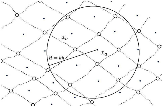
Figure 1. Schematic drawing illustrating the SPH interpolation in two-space dimensions (n = 2). The circle of radius H = kh defines the compact support of the kernel function W(|xa − xb|, h) centered at the position xa of the observation particle a. Although the particles are depicted as point-like masses, their geometrical shape corresponds to an irregular rectangular cell of area mb/ρb. Due to the Lagrangian nature of SPH, the rectangles deform during the evolution. However, they do not overlap and do not have empty interstices between them, which is consistent with the requirement that mb/ρb ≠ 0.
2.4. Scaling Laws and Resolution of the SPH Interpolation
In most SPH simulations it has been a common practice to fix the resolution by simply choosing the value of h as a factor of the interparticle distance. However, Zhu et al. [12] derived scaling relations complying with the resolution limit h → 0 when N → ∞. If a kernel of compact support is employed, then full consistency for the SPH interpolation is achieved when the limit (xa, h) → ∞ is also satisfied. Only when this joint limit is met the particle approximation, defined by Equation (8), converges locally to the kernel approximation, defined by Equation (6).
According to Equation (9) and for a non-uniform distribution of particles, the limit (xa, h) → ∞ is achieved for h → 0 if the mass, m(xa, h), of particles scales with h as hβ with β > n [14]. Consequently, a local scaling law is obtained for the number of neighbors (xa, h) within the compact support Ωn,a of the kernel as
This is the same scaling law obtained by Zhu et al. [12] for the case when n = 3. A global scaling law for the total number of particles N is obtained by invoking a relation of similarity between the average particle density in the compact support Ωn,a of the kernel and the particle density in the full computational domain of total volume V:
Since the volume V of the computational domain does not depend on the parameters of the SPH interpolation, the global scaling law is obtained as follows
which complies with the joint limit for full particle consistency.
3. SPH Convergence Theorem
A measure-value formulation was used by Evers et al. [13] to prove the convergence of SPH as a special case of a class of approximating measures that is much broader than just a sum of weighting kernel functions. In their case the proof was obtained in the limit when N → ∞ for kernel functions of extended support. Here we generalize the measure-value formulation implemented by Evers et al. [13] to prove the theorem of SPH convergence for kernel functions of locally finite support , where y is the coordinate in a Eulerian description. The analysis applies equally well to regularly and irregularly distributed particles. For a fixed instant of time t ∈ [0, T], where T defines the evolution time, the compact support of the kernel will be denoted by Ωy,t. Motion mapping, y = Φ(x, t), is invoked (with the initial condition x = Φ(x, 0)), in order to transform from Eulerian (y) to Lagrangian (x) coordinates (see Equation 2).
3.1. SPH Interpolation in the Context of Measure Theory
In the context of measure theory, the mass differential ρ(y, t)dny is associated with the measure for a given time t, while at time t = 0 the mass differential ρ(x, 0)dnx is associated to the measure . Therefore, the kernel approximation for the mass density of the fluid is
In this regularization process the kernel function W(|y − y′|, h) has compact support Ωy,t and meets the conditions listed in Section 2.2. Note that the regularized density depends on the smoothing length h. If we invoke the motion mapping y = Φ(x, t) (or motion push-forward) in the context of measure theory, then the kernel approximation of the mass density becomes
Equation (16) for is a functional of μt(•), while Equation (17) for is a functional of Φ(x, t).
The particle approximation is obtained by substituting the measure μ0(•) by the discrete measure so that
where the mass mb of particle b scales with h as hβ, with β > n [14]. The discrete measure is constructed using the Dirac delta measures δ0,xb(t) centered at xb(t), which evolve according to the push-forward motion, xb(t) = Φ(xb, t), with xb(0) = xb. Substitution of the initial discrete measure given by Equation (18) into the Lagrangian L(t) of the continuous system given by Equation (3) and in the regularized density defined by Equation (17), we obtain the discrete version of the Lagrangian for a system of point masses as it applies to the traditional SPH method [17, 22], i.e.,
with
where N is the total number of particles that discretize the computational volume and (xa(t), h) is the number of neighbors within the compact support of the kernel W(|xa(t) − xb(t)|, h) centered at the position xa(t) of the observation particle a.
3.2. The Limit When N → ∞
In order to compute the limit of the discrete measure when N → ∞ it is necessary to define eigenobjects in the measure theory, such as the push-forward, the joint representation, and the Wasserstein distance [13].
Definition 3.1 (Push-forward). For a map Φ:A1 → A2 between two measurable spaces (A1, σ1) and (A2, σ2) the push-forward for the measure is the measure that is constructed by means of the map Φ:
or in its integral form
where the map Φ defines the change of coordinates y = Φ(x, t).
The push-forward definition contains the change of variables in the integration methods, as observed in the change from the Eulerian to the Lagrangian representation through the motion mapping y = Φ(x, t) (see Equations 1–3, 16, and 17). In particular, the particle approximation can be expressed as
with
where ΔVb is the volume of particle b and xb is its position. Then
with .
Note that for all x ∈ V there always exists b that belongs to the set of labels {1, 2, …, N} such that
For bounded V, there exists α ∈ ℝ+ such that Δsup = αΔmean, where Δsup is the maximum distance between all pairs of particles Δ(xa, xb) for a, b = 1, 2, …, N. In the present analysis we consider the parameter α of the distribution of particles and not of the total number of particles N. This is consistent with the similarity relationship (14).
The partition of unity as introduced by Sigalotti et al. [14] can be expressed in the context of measure theory. Let n,a be the spherical volume of the compact support Ωn,a of the kernel function , centered at position xa and with smoothing length h, then the partition of unity can be written as
where the domain of integration is taken over the volume of the kernel support. When passing from the smoothed to the particle approximation, the partition of unity will then take the form [14]:
where (xa, h) is the number of neighbors that belong to Ωn,a and ΔVb = mb/ρ(xb) is the volume of particle b located at the point xb, with xb ∈ Ωn,a. In the particle approximation the partition of unity is reproduced only approximately to order O(hn+2). In Figure 1, where the kernel support is represented schematically in the plane (n = 2), the partition of unity deviates from one due to those particle volumes that are intersected by the circular compact support.
Definition 3.2 (Joint representation). Let two measures be and of a space of measure (A, σ). The joint representation of μ1 and μ2 is the measure π:σ × σ → 0∪ℝ+ such that
Definition 3.3 (Wasserstein distance). Let Π(μ1, μ2) be the set of all joint representations of μ1 and μ2. The Wasserstein distance between two measures μ1 and μ2 of a measurable space (A, σ) is
Using Equation (21), the Wasserstein distance between the discrete measure and the continuous measure μ0 is
In the limit N → ∞, the result of Evers et al. [13] is obtained from the above inequality provided that the similarity relation (14) holds. Hence
and therefore taking the limit when N → ∞ gives
Furthermore, if we add the necessary requirement to satisfy the global scaling (15), we immediately find that
so that in the limit when h → 0
3.3. Dynamics of the Regularized Continuous System
According to Evers et al. [13] the Lagrangian L(t) (see Equation 3) is regularized as follows. First, ρ(x, 0)dnx is replaced by μ(dnx) and then the density is regularized according to Equation (17) for , where now the kernel function W(|Φ(x, t) − Φ(x′, t)|, h) has compact support initially centered at x.
The dynamics of the regularized system is obtained by generalizing the principle of least action [13]. The dynamics obtained this way describe the evolution of two fields: the trajectory of the material point Φ(x, t) and the measure μt. The dynamic state is well-defined if the initial position of each material point, namely Φ(x, 0) = x, its initial velocity field , and the initial measure μ0, which is associated with the geometry of the space where the continuous system evolves, are all known.
Then the dynamical system to be described is:
Given T > 0, we have a V ⊂ ℝn and a σ-algebra, denoted by Σ, of the set V with the initial measure μ0 over the Measurable Space (V, Σ) that satisfies μ0 : Σ → [0, +∞) and an initial velocity field . The evolution is then governed by the following set of equations
For all x ∈ V and all t ∈ (0, T] the notation Wh * μt emphasizes that the evolution in the regularization is caused by the push-forward Φ(x, t) # μ0, where U ∈ C2(ℝn; ℝ) is the potential due to external fields. The internal energy e(ρ) ∈ C2(ℝ+; ℝ) is associated only with the thermodynamic properties of the continuum, with e(ρ, y) = U(y)+e(ρ). The field η ∈ C1(ℝn ℝ+) describes the viscosity and the field K ∈ C1(ℝn ℝn) represents a non-local internal interaction in the continuous system.
3.4. The Theorem of Existence-Uniqueness and Continuity With Respect to the Initial Conditions
The main theorem of Evers et al. [13] ensures that the regularized dynamical system given by Equation (29), with the initial conditions of Φ(x, 0) = x and , has a unique solution (μt, Φ(x, t)) for all x ∈ V and t ∈ (0, T], if the initial measure μ0 is known. Also the solutions of Equation (29) are continuous with respect to the initial measure. The following theorems hold:
Theorem 3.1 (Existence-uniqueness). For all t ∈ (0, T], let h > 0 and the initial conditions Φ(x, 0) = x and known for the regularized continuous system of Equation (29). Then for each initial measure μ0 over the measurable space (V, Σ) there is a unique pair solution (μt, Φ(x, t)) to the dynamical system defined by Equation (29).
Theorem 3.2 (Continuity with respect to μ0). For all t ∈ (0, T], let be h > 0 and the initial conditions Φ(x, 0) = x and known for the regularized continuous system of Equation (29). Given two initial measures and over the measurable space (V, Σ), the supremum of the Wasserstein distance between the two solutions and of the regularized dynamical system given by Equation (29) is bounded by:
where M4 and M5 are both positive and independent of the initial measurements and .
Corollary 3.1 (Convergence of the particle approximation to the smoothing approximation). For all t ∈ (0, T], let be h > 0 and the initial conditions be Φ(x, 0) = x and known for the regularized continuous system of Equation (29). Consider a sequence of initial discrete measures over the measurable space (V, Σ) that converge to measure μ0 over (V, Σ), then
For each sequence of initial discrete measures, , there is a unique sequence solution of the dynamical system given by Equation (29). Let (μt, Φ(x, t)) be the solution of the dynamical system of Equation (29) with initial conditions (μ0, Φ(x, 0)). Then converges to μt as
Remark (On the convergence of the particle approximation to the kernel approximation when h → 0). Corollary 3.1 ensures that in the limit h → 0 the SPH particle approximation, ΦSphPA (see Equation 20), converges to the kernel approximation. This is true if the local scaling law (13) and the similarity relation (14) are satisfied [or equivalently, the similarity relation (14) and the global scaling law (15) are both satisfied].
4. Analytical Proof of Convergence
Full consistency of the particle approximation is guaranteed only when the joint limit N → ∞, h → 0 and → ∞ is achieved [12]. Previous studies on the SPH consistency were mostly based on how well the discrete kernel normalization condition is reproduced [12, 14]. For low discrepancy sequences of particles, the standard deviation of the density field approximately varies as −1 when is larger than about 200 [12]. According to Corollary 3.1, the Wasserstein distance can be used to measure how the particle approximation converges to the continuous kernel approximation. Let us first consider the case of an n-dimensional system of volume V, for which the kernel approximation is implemented using a non-local kernel function (i.e., without compact support). The Wasserstein distance between a discrete measure and a continuous measure μt can be estimated from its upper bound given by Equation (25) as
If, on the other hand, the kernel approximation is implemented using an interpolation function of compact support, from Equation (27) it follows that
From the triangular inequality, the convergence properties of , with t ∈ [0, T], can be studied by assessing that is a Cauchy sequence, that is
where N2 > N1 → ∞. Numerical calculations to assess that is a Cauchy sequence under the Wasserstein distance must require using finite linear programming techniques. However, the numerical calculation of the Wasserstein distance is a rather hard task because the computational complexity scales poorly as N. According to Panaretos and Zemel [24], the best algorithms to compute the optimal solution have the prohibitive complexity N3logN. Therefore, a proper numerical three-dimensional test showing the SPH convergence in terms of the Wasserstein distance for high values of N and and sufficiently low values of h will be the subject of a further research paper in this line.
When the SPH interpolation is performed using a kernel function of compact support, the Wasserstein distance between discrete measures, namely and , for k ≫ 1 is given asymptotically by the relation
while the convergence rate for an n-dimensional system is given by
where n is the dimension of the Euclidean space ℝn. In particular, Evers et al. [13] have obtained numerically the convergence rate for n = 1 and 2, but using SPH parameters, i.e., low values of N and h, for which consistency cannot be guaranteed.
For a kernel function of a compact support, the Wasserstein distance between the two discrete measures and approaches asymptotically the form
for β > n when Δh ≪ h → 0. Hence, the rate of convergence obeys the relation
which embodies a rather slow convergence even when Δh/h < < 1 and h → 0.
5. Conclusions
In this paper the formulation introduced by Evers et al. [13] to prove the convergence of the method of Smoothed Particle Hydrodynamics (SPH) in the Wasserstein distance of the corresponding measure-valued evolutions is extended to kernel functions of locally finite support and irregular particle distributions. The present analysis has demonstrated the convergence and consistency of SPH in the joint limit h → 0 and N → ∞. In this limit consistency of the particle approximation solution of the equations of motion of the regularized continuum system is obtained when the number of neighbors within the compact support of the kernel, , tends simultaneously to infinity, albeit at a rate slower than N so that /N → 0. It is important to recall that, in contrast to previous proofs of SPH convergence in the framework of measure theory, here the continuous system considered is regularized by means of a kernel function of compact support. The particle approximation of the exact differential equations has been done in compliance with the similarity relation / = N/V, where is the volume enclosed by the kernel support and N is the total number of particles that discretize the computational domain, and the global scaling law N ~ h−β for β > n, where h is the smoothing length and n is the dimension of the Euclidean space ℝn. Convergence is also achieved if the above global scaling law is replaced by the local scaling ~ hn − β for β > n, as was first derived by Zhu et al. [12] and later on by Sigalotti et al. [14] following different methodologies. Since most modern SPH simulations employ interpolation functions of compact support, the present analysis demonstrate that in the most favorable case when both N → ∞ and h → 0 simultaneously, then full consistency is achieved only when also → ∞.
Data Availability Statement
The original contributions presented in the study are included in the article/supplementary material, further inquiries can be directed to the corresponding author.
Author Contributions
OR, GA, JK, LS, and CV have contributed intellectually to the form and content of this manuscript. The writing was done by OR and LS. All authors agree with the version submitted for publication, contributed to the article, and approved the submitted version.
Funding
We acknowledge funding from the European Union's Horizon 2020 Programme under the ENERXICO Project, grant agreement No. 828947 and from the Mexican CONACYT-SENER Hidrocarburos Programme under grant agreement B-S-69926.
Conflict of Interest
The authors declare that the research was conducted in the absence of any commercial or financial relationships that could be construed as a potential conflict of interest.
Publisher's Note
All claims expressed in this article are solely those of the authors and do not necessarily represent those of their affiliated organizations, or those of the publisher, the editors and the reviewers. Any product that may be evaluated in this article, or claim that may be made by its manufacturer, is not guaranteed or endorsed by the publisher.
Acknowledgments
We acknowledge financial support from the Departamento de Ciencias Básicas of the Universidad Autónoma Metropolitana - Azcapotzalco through internal funds.
References
1. Gingold RA, Monaghan JJ. Smoothed particle hydrodynamics: theory and application to non-spherical stars. Monthly Not R Astron Soc. (1977) 181:375–89. doi: 10.1093/mnras/181.3.375
2. Lucy LB. A numerical approach to the testing of the fission hypothesis. Astron J. (1977) 82:1013–24. doi: 10.1086/112164
3. Sayeb M, Blecha L, Kelley LZ, Gerosa D, Kesden M, Thomas J. Massive black hole binary inspiral and spin evolution in a cosmological framework. Monthly Not R Astron Soc. (2020) 501:2531–46. doi: 10.1093/mnras/staa3826
4. Lind SJ, Stansby PK. High-order Eulerian incompressible smoothed particle hydrodynamics with transition to Lagrangian free-surface motion. J Comput Phys. (2016) 326:290–311. doi: 10.1016/j.jcp.2016.08.047
5. Di Lisio R, Grenier E, Pulvirenti M. On the regularization of the pressure field in compressible Euler equations. Annali della Scuola Normale Superiore di Pisa, Classe di Scienze 4e. (1997) 24:227–38.
6. Di Lisio R, Grenier E, Pulvirenti M. The convergence of the SPH method. Comput Math Appl. (1998) 35:95–102. doi: 10.1016/S0898-1221(97)00260-5
7. Ben Moussa B, Vila JP. Convergence of SPH method for scalar nonlinear conservation laws. SIAM J Num Anal. (2000) 37:863–87. doi: 10.1137/S0036142996307119
8. Quinlan NJ, Basa M, Lastiwka M. Truncation error in mesh-free particle methods. Int J Num Methods Eng. (2006) 66:2064–85. doi: 10.1002/nme.1617
9. Vaughan GL, Healy TR, Bryan KR, Sneyd AD, Gorman RM. Completeness, conservation and error in SPH for fluids. Int J Num Methods Fluids. (2008) 56:37–62. doi: 10.1002/fld.1530
10. Read JI, Hayfield T, Agertz O. Resolving mixing in smoothed particle hydrodynamics. Monthly Not R Astron Soc. (2010) 405:1513–30. doi: 10.1111/j.1365-2966.2010.16577.x
11. Fatehi R, Manzari MT. Error estimation in smoothed particle hydrodynamics and a new scheme for second derivatives. Comput Math Appl. (2011) 61:482–98. doi: 10.1016/j.camwa.2010.11.028
12. Zhu Q, Hernquist L, Li Y. Numerical Convergence in smoothed particle hydrodynamics. Astrophys J. (2015) 800:6. doi: 10.1088/0004-637X/800/1/6
13. Evers JHM, Zisis IA, van der Linden BJ, Duong MH. From continuum mechanics to SPH particle systems and back: Systematic derivation and convergence. J Appl Math Mech. (2018) 98:106–133. doi: 10.1002/zamm.201600077
14. Sigalotti LDG, Rendon O, Klapp J, Vargas CA, Cruz F. A new insight into the consistency of the SPH interpolation formula. Appl Math Comput. (2019) 356:50–73. doi: 10.1016/j.amc.2019.03.018
15. Liu MB, Liu GR. Restoring particle consistency in smoothed particle hydrodynamics. Appl Num Math. (2006) 56:19–36. doi: 10.1016/j.apnum.2005.02.012
16. da Silva LP, Marchi CH, Maneguette M, Foltran AC. Robust RRE technique for increasing the order of accuracy of SPH numerical solutions. Math Comput Simul. (2022) 199:231–52. doi: 10.1016/j.matcom.2022.03.016
17. Monaghan JJ. Smoothed particle hydrodynamics. Rep Prog Phys. (2005) 68:1703–59. doi: 10.1088/0034-4885/68/8/R01
18. Price DJ. Smoothed particle hydrodynamics and magnetohydrodynamics. J Comput Phys. (2012) 231:759–94. doi: 10.1016/j.jcp.2010.12.011
19. Landau LD, Lifshitz EM. Fluid Mechanics. Volume 6 of Course of Theoretical Physics. Oxford: Pergamon Press (1987).
20. Lind SJ, Rogers BD, Stansby PK. Review of smoothed particle hydrodynamics: towards converged Lagrangian flow modelling. Proc R Soc A Math Phys Eng Sci. (2020) 476:20190801. doi: 10.1098/rspa.2019.0801
21. Liu GR, Liu MB. Smoothed Particle Hydrodynamics: A Meshfree Particle Method. Singapore: World Scientific (2003) doi: 10.1142/9789812564405
22. Dehnen W, Aly H. Improving convergence in smoothed particle hydrodynamics simulations without pairing instability. Monthly Not R Astron Soc. (2012) 425:1068–82. doi: 10.1111/j.1365-2966.2012.21439.x
23. Fulk DA, Quinn DW. An analysis of 1-D smoothed particle hydrodynamics kernels. J Comput Phys. (1996) 126:165–80. doi: 10.1006/jcph.1996.0128
Keywords: particle method, SPH interpolation, consistency, scaling laws, similarity relation, convergence of the SPH method, measure theory, Wasserstein distance
Citation: Rendón O, Avendaño GD, Klapp J, Sigalotti LDG and Vargas CA (2022) Local Consistency of Smoothed Particle Hydrodynamics (SPH) in the Context of Measure Theory. Front. Appl. Math. Stat. 8:907604. doi: 10.3389/fams.2022.907604
Received: 29 March 2022; Accepted: 23 May 2022;
Published: 22 June 2022.
Edited by:
José Tadeu Lunardi, Universidade Estadual de Ponta Grossa, BrazilReviewed by:
Luciano Pereira Da Silva, Universidade Federal Do Paraná (UFPR), BrazilAppanah Rao Appadu, Nelson Mandela University, South Africa
Copyright © 2022 Rendón, Avendaño, Klapp, Sigalotti and Vargas. This is an open-access article distributed under the terms of the Creative Commons Attribution License (CC BY). The use, distribution or reproduction in other forums is permitted, provided the original author(s) and the copyright owner(s) are credited and that the original publication in this journal is cited, in accordance with accepted academic practice. No use, distribution or reproduction is permitted which does not comply with these terms.
*Correspondence: Otto Rendón, b3R0b3JlbmRvbkBnbWFpbC5jb20=