Log-Linear Model and Multistate Model to Assess the Rate of Fibrosis in Patients With NAFLD

In this paper, the deleterious effects of obesity, type II diabetes, and insulin resistance, systolic and diastolic hypertension on the rate of progression of fibrosis in patients with non-alcoholic fatty liver disease (NAFLD) are illustrated using a new approach utilizing the Poisson regression to model the transition rate matrix. The observed counts in the transition count matrix are used as the response variables and the covariates are the risk factors for fatty liver. Then, the estimated counts from running the Poisson regression are used to estimate the transition rates using the continuous-time Markov chains (CTMCs) followed by exponentiation of the estimated rate matrix to obtain the transition probability matrix at specific time points. A depicted, hypothetical, observational, prospective longitudinal study of 150 participants followed up every year for a total of 29 years recording their demographic characteristics and their timeline follow-up is demonstrated. The findings revealed that insulin resistance expressed by HOMA2-IR had the most deleterious effects among other factors on increasing the rate of fibrosis progression from state 1 to state 2, from state 2 to state 3, and from state 3 to state 4. The higher the level of HOMA2-IR is, the more rapid the rate of progression is. This analysis helps the health policymakers and medical insurance managers to allocate the financial and human resources for investigating and treating high-risk patients with NAFLD. In addition, this analysis can be used by pharmaceutical companies to conduct longitudinal studies to assess the effectiveness of the newly emerging anti-fibrotic drugs.

Introduction

Continuous-time Markov chains (CTMCs) are valuable mathematical and statistical tools. They are of great potential to evaluate the disease progression over time. NAFLD is an increasingly worldwide epidemic, paralleling the rise in the incidence of obesity and type II diabetes which are approaching a pandemic level. This emerging health problem is mainly due to sedentary life styles and western eating habits of ingesting high-fat and cholesterol diets. The pathological milestone for NAFLD is insulin resistance and hyperinsulinemia. This hyperinsulinemia will eventually result in type II diabetes with adverse complications like vascular diseases and fatty liver disease. On the other hand, NAFLD can cause type II diabetes, as the prevalence of diabetes in NAFLD ranges between 18 and 45%. Moreover, the prevalence of NAFLD in type II diabetic patients ranges between 49 and 75% [1].

Non-alcoholic fatty liver disease can be modeled using the simplest form for health, disease, and death model. It is composed of four states. One state is for susceptible individuals with risk factors like type II diabetes, dyslipidemia, obesity, and hypertension. The second state is the NAFLD phenotypes. The other two competing states for death are: one for liver-related mortality as a complication of NAFLD and the other state is the death causes unrelated to liver disease [2]. This model is shown in Figure 1.

FIGURE 1

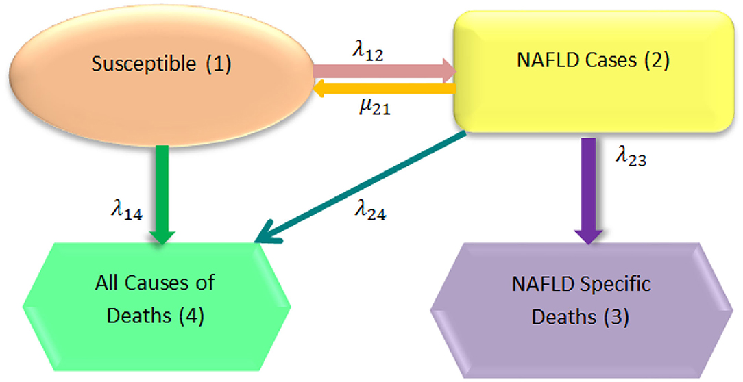
Figure 1. General model structure [2].

In addition, NAFLD can be modeled in more elaborate expanded form which includes nine states [3]. The first eight states are the states of disease progression over time and the ninth state is the death state [2], as illustrated in Figure 2.

FIGURE 2

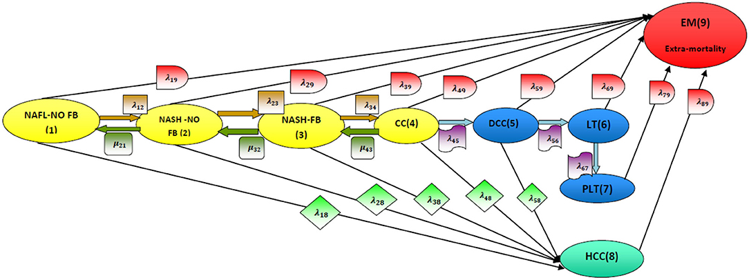
Figure 2. Disease model structure [2]. NAFL-NO FB, non-alcoholic fatty liver with no fibrosis (stage 1); NASH-NO FB, non-alcoholic steatohepatitis with no fibrosis (stage 2); NASH-FB, non-alcoholic steatohepatitis with fibrosis (stage 3); CC, compensated cirrhosis (stage 4); DCC, de-compensated cirrhosis (stage 5); LT, liver transplant (stage 6); PLT, post-liver transplant (stage 7); HCC, hepatocellular carcinoma (stage 8); EM, extramortality (stage 9).

Moreover, fibrogenesis is a dynamic process that goes back and forth among the early stages of the expanded model. Stages of fibrous tissue formation are early seen in NAFLD process. Fibrosis progresses if the risk factors for its formation are not eliminated. Fibrosis is an ominous sign for loss of liver functions. When the fibrous tissue develops, a subset of the early states is used to relate these risk factors to the rates. Definition of each state is shown in Figure 3 [4, 5]. F0 indicates that there is no fibrous tissue. F1 means that fibrous tissue is deposited due to non-alcoholic steatohepatitis (NASH) and not due to any other causes of liver disease; all other stages (F2 and F3) are maintained and are progressing over time by the presence of NASH till the liver cirrhosis (F4). If this NASH is well-treated by controlling the risk factors that induce it, the fibrous tissue formation and deposition will regress as shown in the Figure 3.

FIGURE 3

Figure 3. NAFLD with the evolving fibrosis stages [4]. F0, no fibrosis (stage 0); NASH-FB-1, non-alcoholic steatohepatitis with mild fibrosis (stage 1); NASH -FB-2, NASH with moderate fibrosis (stage 2); NASH -FB-3, NASH with advanced or severe fibrosis (stage 3); CC, compensated cirrhosis (stage 4) which is the more severe or advanced form of fibrosis.

Kalbfleisch and Lawless [6] related the instantaneous rate of transitions from state i to state j to covariates, by regression modeling of the Q transition rate matrix using log-linear model for the Markov rates.

The previous studies, as will be later mentioned in the discussion, mainly included the evaluation of 2 paired biopsies, initial and second biopsies, then grouping the patients according to the findings into stable, regressors, slow progressors, and rapid progressors without precise estimation of specific transition rates among states and without proper estimation of the predictive value of each variable on these specific rates. The rate of fibrosis progression was estimated by dividing the difference in fibrosis stage between biopsies by the time interval (in years), and this was performed to account for the time differences between the biopsies [7]. Additionally, either univariate or multivariate linear regression was used to relate the risk factors with the rate of progression. As will be later mentioned in the discussion, some studies utilized multivariate logistic regression instead of linear regression.

This depicted study differs from the previous studies in many aspects. First, it proposes recording multiple repeated observations over time. Second, it suggests running Poisson regression to relate the transition rates among states with the risk factors. Third, it recommends using continuous-time Markov chains to obtain the transition probabilities and predict the expected counts of patients in each state at a specific time point in the future. The counts of each transition can be modeled as a function of some explanatory variables reflecting the characteristics of the patients. The Poisson regression model specifies that each response y_i is drawn from a Poisson population with parameter λ_i, related to the covariates. The primary equation of the model is

$\begin{array}{l}P(Y=y_i|X_i)=\frac{exp(-{\lambda }_i){\times \lambda }_i^{y_i}}{y_i!}.\end{array}$

The most common formulation for the λ_i is the log-linear model:

$\begin{array}{l}ln{\lambda }_i=X_i^{\prime }\beta =b_0+b_1{x}_{i1}+b_2{x}_{i2}+b_3{x}_{i3}+\dots .+b_k{x}_{im}.\end{array}$

where β is the k × 1 parameter vector, m is the number of predictors, and Xs are the predictors.

The expected number of events per period is given by:

$\begin{array}{l}E\left[y_i|X_i\right]=var\left[y_i|X_i\right]={\lambda }_i=exp(X_i^{\prime }\beta ).\end{array}$

The observed counts in the transition counts matrix are used as response variables. The covariates are the risk factors for the fatty liver, where the participants are subjected to the same follow-up periods. Then, the estimated counts obtained from running the Poisson regression are used as input to estimate the transition probability matrix using the CTMC. The author clarifies this procedure using a hypothetical example in the form of an observational prospective longitudinal study.

Attia [8] used the same data in previous work. Still, in this article, the author discusses the issue of multicollinearity, the equidispersion Poisson of response variables in the presence of excess zeros, and more comparisons between this work and previous works. Finally, the author highlights the benefit of such analysis to pharmacoeconomic evaluation and healthcare economics.

Materials and Methods

Patients

A total of one hundred fifty participants were followed up every year for 29 years, and during each visit, the characteristics of the participants were recorded like sex (0 = female, 1 = male), age, body mass index (BMI), low-density lipoprotein (LDL)-chol, homeostatic model assessment-insulin resistance (HOMA2-IR), and systolic blood and diastolic blood pressure. For each participant, the recorded value is the mean of the follow-up measurements. The age is the median value. The participants were followed up till the end of the study or having liver cirrhosis (F4).

Statistical Analysis

The relationship between the response variable (counts of transitions) and the predictors was non-linear as shown by Lowess smoother. Restricted cubic spline was used to obtain a suitable functional form of the predictors to fit a Poisson model using STATA 14. The CTMCs were used to obtain transition probability matrix and transition rate matrix. p-Value of <0.05 was considered statistically significant; all tests were two-sided tests (refer to Appendix A).

Results

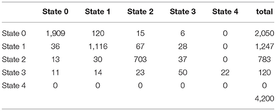
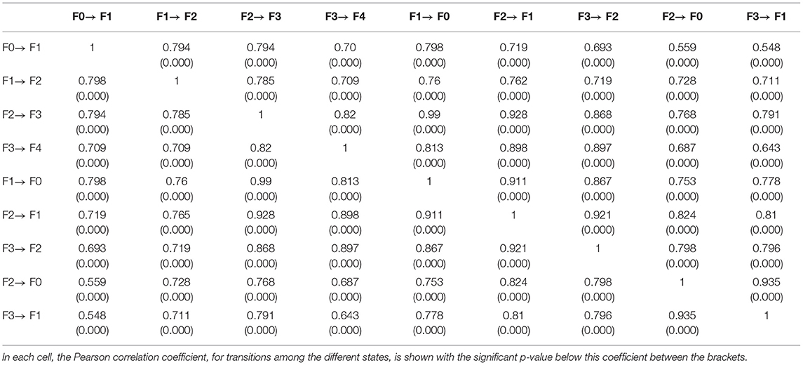
Summary of the transition counts among the states is shown in Table 1. The observed counts of the participants over the 29 years of follow-up are demonstrated in Table 2. The distribution of these counts was Poisson (mean = variance). The dispersion indices for the nine response variables ranged between 0.82 and 1.34. In Appendix B, more figures illustrate the dispersion of these response variables. They were also correlated with high statistical significance (p-value = 0.000) as shown in Table 3.

TABLE 1

Table 1. Summary of transition counts among the states.

TABLE 2

Table 2. Observed transition counts of the patients over the 29 years.

TABLE 3

Table 3. Correlation between the different response variables.

Initial observed rates are as follows:

$\begin{array}{l}{\lambda }_{01}=\frac{120}{2050}=0.059,{\lambda }_{12}=\frac{67}{1247}=0.0537,\\ {\lambda }_{23}=\frac{37}{783}=0.047,{\lambda }_{34}=\frac{22}{120}=0.183\\ {\mu }_{10}=\frac{36}{1247}=0.0288,{\mu }_{21}=\frac{30}{783}=0.0383,\\ {\mu }_{32}=\frac{23}{120}=0.191,{\mu }_{20}=\frac{13}{783}=0.016,\\ {\mu }_{31}=\frac{14}{120}=0.116\end{array}$

Although the response counts showed excess zeros, they fitted Poisson distribution and the zero inflated Poisson model. Their mean and variance were approximately equal as evident by their dispersion indices. So, Poisson regression was conducted for each transition count. Most statistical software packages conduct Poisson regression or generalized linear model utilizing log-link function with only one response variable. Thus, using STATA14, Poisson regression was conducted with one response variable. The response variable could not be used as a matrix to conduct the regression as multivariate regression with multiple response variables.

The application of Lowess smoother showed the non-linear relationship between the predictors and the response variables as shown in Figure 4. In Supplementary Materials, more figures illustrating these relationships between the different predictors and response variables are clearly shown (refer to also Appendix B).

FIGURE 4

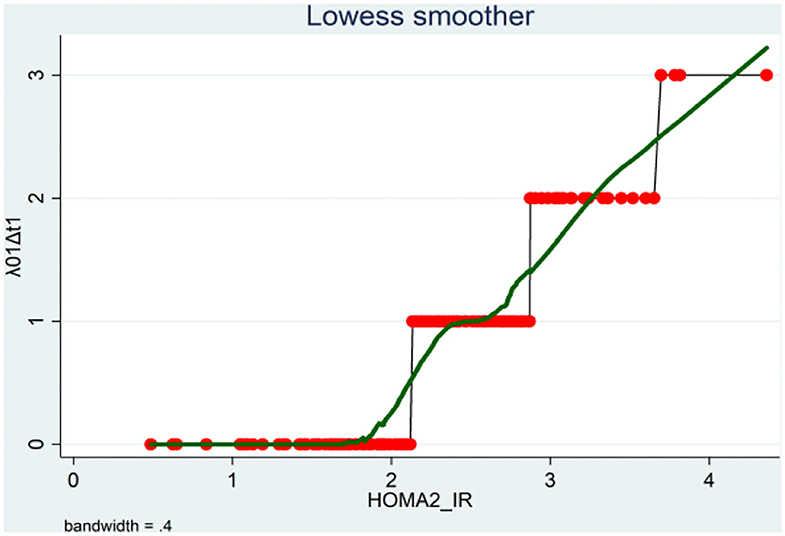
Figure 4. Lowess smoother showing the non-linear relationship between the transition counts from F0 to F1 and the HOMA2-IR levels.

The continuous predictors (age, BMI, HOMA2-IR, LDL-chol, and systolic and diastolic blood pressure) were highly correlated with a correlation coefficient of 0.99 and a condition number for data matrix (X'X) of 453.57. The condition number for the data matrix (X'X) constructed from the transformed variables used in the analysis (HOMAsp1, HOMAsp2, LDLsp2, sysPS2, diasPS2) was 54.89. These transformed variables were also highly correlated. However, the condition number did not exceed 100. Thus, this multicollinearity can be considered non-harmful, and it will not affect the analysis [9].

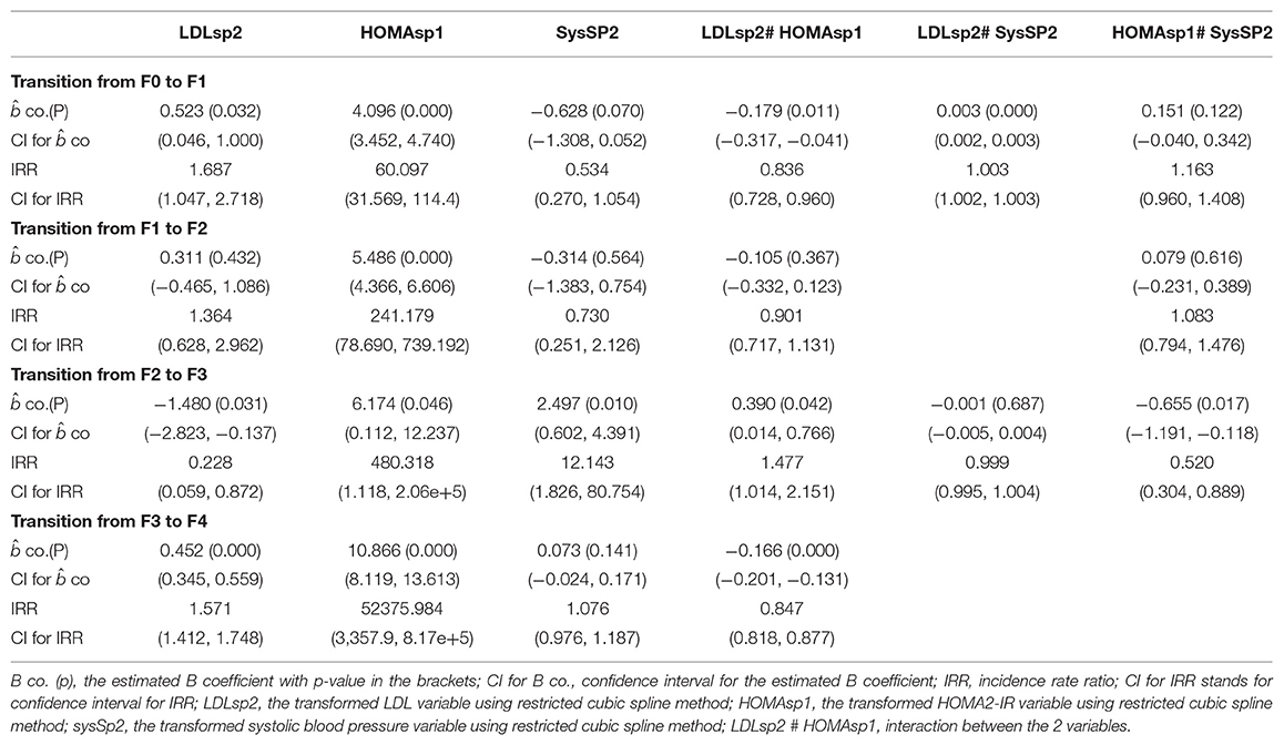
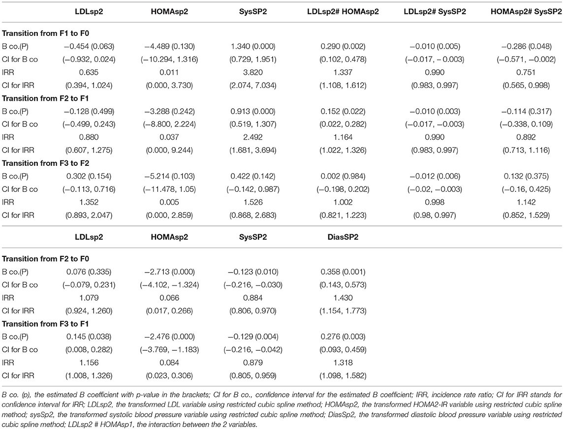
The observed counts were the response variables used to fit the Poisson regression model. For each transition count, the model that represented the most explainable covariates with their estimated beta coefficients and the corresponding incidence rate ratios were illustrated in Appendix B. The transitions were subdivided into progressive transitions and regressive transitions. The main important result is that HOMA2-IR is positively correlated with all progressive transitions and is inversely related to the regressive transitions, with control of other variables, as shown in Tables 4, 5.

TABLE 4

Table 4. Parameters for each transition.

TABLE 5

Table 5. Parameters for each transition.

Progressive Transitions With Rates λ₀₁, λ₁₂, λ₂₃, λ₃₄

Persons with high insulin resistance (elevated HOMA2-IR) had 60 times the rate of transition from F0 to F1 compared to persons with normal level of HOMA2-IR (persons with normal insulin sensitivity), also the rate increased to 240 times for the rate of transition from F1 to F2, increased to 480 times for the rate of transition from F2 to F3, and increased to more than 50,000 times for the rate of transition from F3 to F4. Statistically speaking, the expected increase in log count of transition from F0 to F1 for one-unit increase in transformed HOMA is 4.096, which is highly statistically significant (p = 0.000). The expected increase in log count of transition from F1 to F2 for one-unit increase in transformed HOMA is 5.486, which is highly statistically significant (p = 0.000). The expected increase in log count of transition from F2 to F3 for one-unit increase in transformed HOMA is 6.174, which is not highly statistically significant (p = 0.046). The expected increase in log count of transition from F3 to F4 for one-unit increase in transformed HOMA is 10.866, which is highly statistically significant (p = 0.000).

Regressive Transitions With Rates μ₁₀, μ₂₁, μ₃₂, μ₂₀, μ₃₁

Persons with high insulin resistance (elevated HOMA2-IR) had 0.011 times the rate of transition from F1 to F0 compared to persons with normal level of HOMA2-IR (persons with normal insulin sensitivity), also the rate decreased to 0.037 times for the rate of transition from F2 to F1, decreased to 0.005 times for the rate of transition from F3 to F2, decreased to 0.066 times for the rate of transition from F2 to F0, and decreased to 0.084 times for the rate of transition from F3 to F1. Statistically speaking, the expected decrease in log count of transition from F1 to F0 for one-unit increase in transformed HOMA is 4.489, which is not statistically significant (p = 0.13). The expected decrease in log count of transition from F2 to F1 for one-unit increase in transformed HOMA is 3.288, which is not statistically significant (p = 0.242). The expected decrease in log count of transition from F3 to F2 for one-unit increase in transformed HOMA is 5.214, which is not statistically significant (p = 0.103). The expected decrease in log count of transition from F2 to F0 for one-unit increase in transformed HOMA is 2.713, which is highly statistically significant (p = 0.000). The expected decrease in log count of transition from F3 to F1 for one-unit increase in transformed HOMA is 2.476, which is highly statistically significant (p = 0.000).

Validation and Residual Analysis

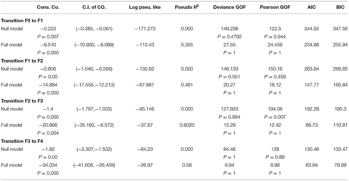
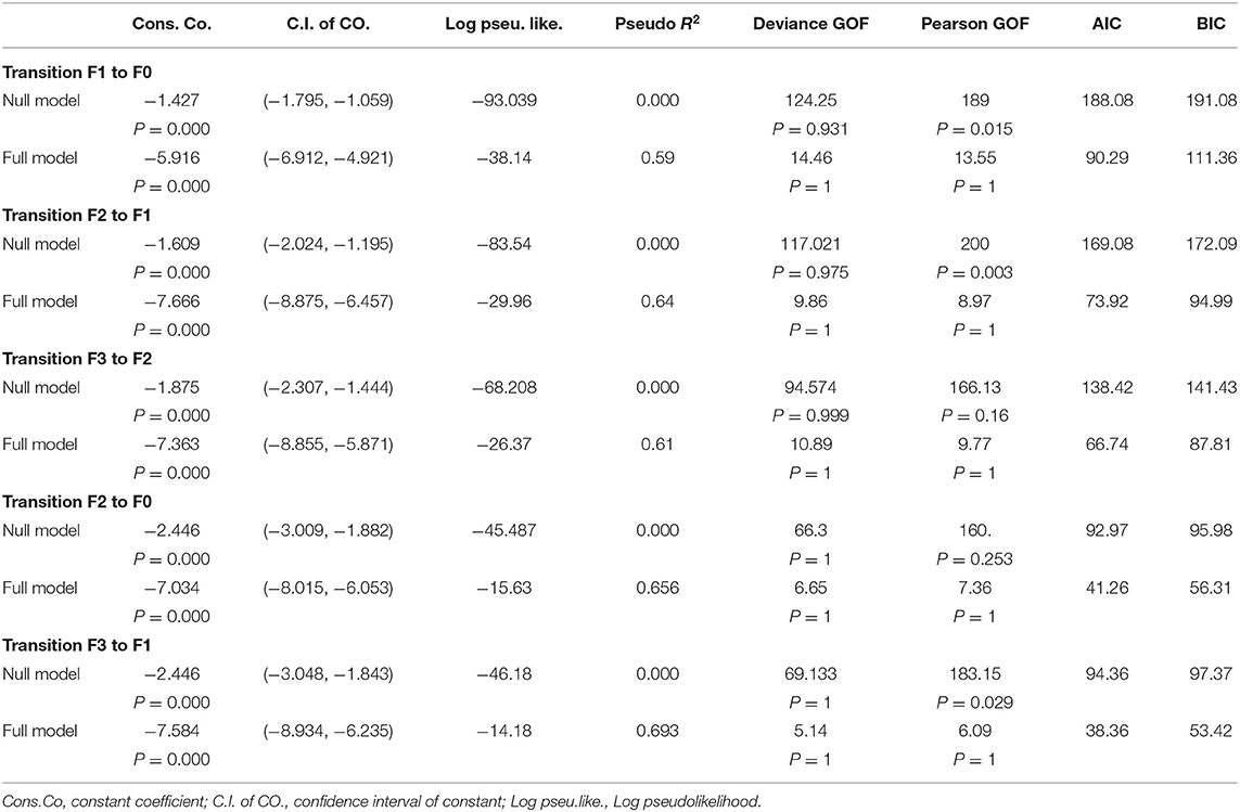
Poisson model fitted the data. When comparing the full model to the null model, there was a marked decrease in the deviance goodness of fit. Also, the akaike information criteria (AIC) and bayesian information criteria (BIC) were less than their values in the null model, indicating the full model improvement. In addition, there was an increase in the pseudo-R², indicating the ability of the model to predict the outcome better than the null model. The output results of the null model for each of the transition counts are shown in Tables 6, 7.

TABLE 6

Table 6. Comparison between null and full model as regards the progressive transitions.

TABLE 7

Table 7. Comparison between null and full model as regards the regressive transitions.

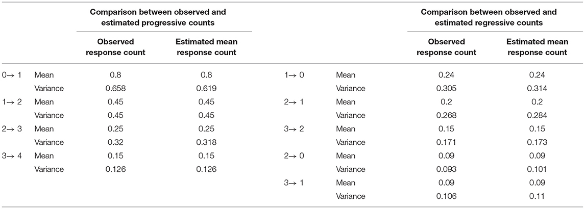
The observed rates were approximately equal to the estimated rates after running the Poisson model as shown in Table 8.

TABLE 8

Table 8. The comparison between observed and estimated response rate after fitting Poisson model.

Analysis of residuals especially Pearson residuals, for all transitions, revealed that they were not normally distributed. The Q-Q plot for these residuals did not exhibit normality. The Pearson dispersion statistics for each count was less than one supporting no evidence of overdispersion of the fitted model despite the apparent excess zeros (Appendix B, Table 21). Generalized Poisson regression did not fit the data. In Appendix C, more figures of these residuals are presented [10, 11].

This observational study aims to obtain preliminary and explanatory ideas about the effects of each risk factor on the different transition counts among the states. This Poisson regression is not aiming for future prediction of counts. Although the residuals are not normally distributed, such analysis can give fair provisional ideas about the effects of the risk factors. The Poisson model gives unbiased estimates for the regression coefficients, but these coefficients' statistical significance should be cautiously taken.

CTMCs Utilize the Estimated Counts From Log-Linear Model to Obtain the Transition Probability Matrix

For each of the transitions from state (i) to state (j), where λ_ij denotes the counts of transition from state (i) to state (j), and after running the Poisson model, the linear predictor $ln{\lambda }_{ij}=X_n^{\prime }B$ for each participant (n) is exponentiated, $E\left[y_n|X_n\right]={\lambda }_{ij}=exp\left(X_n^{\prime }B\right),$to obtain the expected counts of transition that this participant had accomplished during this 29 years. Then, the result is rounded to the appropriate integer and summed to get all counts for this transition and then compared to the observed counts accomplished by all participants.

The n_i+ is the total marginal transition counts out of this state, which is assumed to be constant. The estimated counts from running the Poisson model will be substituted in the transition count table. Because the marginal counts are assumed to be the same and when using the initial rates calculated as ${\theta }_0=\frac{n_{ij}}{n_{i+}}$ where the n_ij is the transition counts from state i to state j, the Q matrix can be estimated. (Hint: the numerators below are the estimated counts obtained from running the Poisson regression).

$\begin{array}{l}\widehat{Q}=\\ \left[\begin{array}{ccccc}-{\lambda }_{01}& {\lambda }_{01}& 0& 0& 0\\ {\mu }_{10}& -\left({\lambda }_{12}+{\mu }_{10}\right)& {\lambda }_{12}& 0& 0\\ {\mu }_{20}& {\mu }_{21}& -\left({\lambda }_{23}+{\mu }_{21}+{\mu }_{20}\right)& {\lambda }_{23}& 0\\ 0& {\mu }_{31}& {\mu }_{32}& -\left({\lambda }_{34}+{\mu }_{32}+{\mu }_{31}\right)& {\lambda }_{34}\\ 0& 0& 0& 0& 0\end{array}\right]\end{array}$

where

$\begin{array}{l}{\lambda }_{01}=\frac{120}{2050}=0.059,{\lambda }_{12}=\frac{64}{1247}=0.051,\\ {\lambda }_{23}=\frac{35}{783}=0.045,{\lambda }_{34}=\frac{20}{120}=0.167\\ {\mu }_{10}=\frac{36}{1247}=0.029,{\mu }_{21}=\frac{26}{783}=0.033,\\ {\mu }_{32}=\frac{19}{120}=0.158,{\mu }_{20}=\frac{12}{783}=0.015,\\ {\mu }_{31}=\frac{13}{120}=0.108\end{array}$

The probability matrix at any specific time point in the future can be obtained by exponentiation of this matrix because the chain is homogenous continuous-time Markov chains with constant rates over time. This result can also be obtained by solving the forward Kolmogorov differential equations, which will yield the same result as the exponentiation of the estimated Q matrix (refer to Appendix D).

The transition probability matrix is obtained by exponentiation of this estimated $\widehat{Q}$ matrix after 1 year:

$\begin{array}{l}P\left(t=1\right)=\exp \left(\widehat{Q}t\right)=\left[\begin{array}{ccccc}{P}_{00}& P_{01}& P_{02}& P_{03}& P_{04}\\ P_{10}& P_{11}& P_{12}& P_{13}& P_{14}\\ P_{20}& P_{21}& P_{22}& P_{23}& P_{24}\\ P_{30}& P_{31}& P_{32}& P_{33}& P_{34}\\ 0& 0& 0& 0& P_{44}\end{array}\right]\\ =\left[\begin{array}{ccccc}0.944& 0.055& 0.001& 0& 0\\ 0.027& 0.925& 0.047& 0.001& 0.0001\\ 0.014& 0.033& 0.915& 0.035& 0.003\\ 0.002& 0.086& 0.125& 0.651& 0.136\\ 0& 0& 0& 0& 1\end{array}\right]\end{array}$

Goodness of Fit for the Multistate Markov Model

To calculate goodness of fit for multistate model used in this example, it is like the procedure used in contingency table:

Step 1: H₀ = future state does not depend on the current state

H₁ = future state depends on the current state

Step 2: After obtaining the estimated Q matrix, the probability matrix is calculated in time interval equals one because the participants' follow-up period was done every year.

$\begin{array}{l}{p}_{ij}\left(\Delta t=1\right)=\exp \left(\widehat{Q}\times \Delta t\right)=\left[\begin{array}{ccccc}{P}_{00}& P_{01}& P_{02}& P_{03}& P_{04}\\ P_{10}& P_{11}& P_{12}& P_{13}& P_{14}\\ P_{20}& P_{21}& P_{22}& P_{23}& P_{24}\\ P_{30}& P_{31}& P_{32}& P_{33}& P_{34}\\ 0& 0& 0& 0& P_{44}\end{array}\right]\\ =\left[\begin{array}{ccccc}0.9435& 0.0551& 0.0014& 0& 0\\ 0.0274& 0.9247& 0.0469& 0.0009& 0.0001\\ 0.0144& 0.0327& 0.9149& 0.0348& 0.0032\\ 0.0023& 0.0863& 0.1245& 0.6512& 0.1357\\ 0& 0& 0& 0& 1\end{array}\right]\end{array}$

Step 3: Calculate the expected counts in this interval.

$\begin{array}{r}{E}_{ij}=n_{i+}{P}_{ij}(t).\\ n_{1+}=2050,n_{2+}=1247,n_{3+}=783,n_{4+}=120\end{array}$

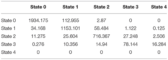
Multiplying each row in the probability matrix with the corresponding total marginal counts in the observed transition counts table in the same interval yields the expected counts as shown in Table 9.

Step 4: The observed counts, O_ij, are shown in Table 2. The expected counts, E_ij, are obtained from the previous step and are shown in Table 9. Then, apply the Pearson statistic formula which yields a value of 1,140.097 with high statistical significance (p = 0.000). Apply $\sum _{i=1}^5\sum _{j=1}^5\frac{{(O_{ij}-E_{ij})}^2}{E_{ij}}=1140.097~{\chi }_{(5-1)(5-1)(.05)}^2$.

TABLE 9

Table 9. The expected transition counts after one year of the follow-up.

So, from the above results, the null hypothesis is rejected while the alternative hypothesis is accepted and the multistate Markov model fits the data, that is to mean, the future state depends on the current state with the estimated transition rates and probability matrices as obtained.

Health Economics

This transition probability matrix can predict the count of patients in each state at specific time point, for example, if a cohort of 6,000 patients with the following number in each state is $\left[\begin{array}{cc}\begin{array}{ccc}3000& 1800& 1020\end{array}& \begin{array}{cc}180& 0\end{array}\end{array}\right]$, after 1 year the predicted counts will be $\left[\begin{array}{cc}\begin{array}{ccc}2895& 1879& 1044\end{array}& \begin{array}{cc}154& 28\end{array}\end{array}\right]$. This count can be achieved by multiplying the initial count distribution of the patients with the transition probability calculated at the required specific time point, $p_{ij}(t)=exp\left(\widehat{Q}t\right)$

$\begin{array}{l}E\left[u_j(t)|u_j(0)\right]={\displaystyle \sum _{j=1,i=1}^5}{u}_j(0)P_{ij}(t)i,j=1,..,5\end{array}$

Let u (0) be the size of patients in a specific state at specific time t = 0. The initial size of patients is U (0) = u_j (0), as there are 4 transient states (F0 to F3) and 1 absorbing state (F4), where u_j (0) is the initial size or the number of patients in state j at time t = 0 given that u₅ (0) = 0, i.e., initial size of patients in state 5 (absorbing state) is zero at initial time point = 0. As the transition or the movement of the patients among states is independent, at the end of the whole time interval (0, t), there will be u_j (t) patients in the transient states at time t, and there will also be u₅ (t)patients in state 5 (F4 = liver cirrhosis) at time t.

In addition, the state probability distribution π (t), which is the probability distribution for each state at a specific time point given the initial probability distribution π (0), can be estimated by applying the following formula:

$\begin{array}{l}\pi (t)=\pi (0)P(t).\end{array}$

In this example, the cohort of 6,000 patients has initial probability distribution of $\left[\begin{array}{cc}\begin{array}{ccc}0.5& 0.3& 0.17\end{array}& \begin{array}{cc}0.03& 0\end{array}\end{array}\right]$, after 1 year, the state probability distribution will be $\left[\begin{array}{cc}\begin{array}{ccc}0.4825& 0.3131& 0.174\end{array}& \begin{array}{cc}0.0257& 0.0046\end{array}\end{array}\right]$.

Pharmaco-economic evaluation can be assessed in three categories: the cost-benefit analysis, the cost-effectiveness analysis, and the cost-utility analysis. The evaluation utilizes the predicted number of patients in each state estimated every year, the state probability distribution predicted every year, the costs of investigations and treatments, and the quality adjusted life years for the patients [12, 13].

This approach differs from the one used by Rustgi et al. [14] who depends on calculating the cost-effectiveness analysis by following a cohort of patients, all starting at the same initial state till death. While in the approach proposed in this article, sampling the population and estimating the transition probability matrix to predict the counts in the future, any cohort of patients can be followed up utilizing the information gained from sampling the high-risk population.

Discussion

The following discussion elucidates the agreements and comparisons between the findings in this study with the findings in the previous one high-lightening the effects of various factors on progression rate of fibrosis in NAFLD patients.

Hui et al. [15] conducted a study on 17 patients who had previous liver biopsy showing evidence of steatosis with or without the presence of necroinflammation and fibrosis. Those patients underwent second liver biopsies with a median of 6 years apart (range: 3.8–8 years). More than half of them developed progressive fibrosis compared to the initial biopsy; because that these patients suffered from steatohepatitis, although there was no significant correlation between the degree of steatohepatitis and the degree of fibrosis between the two biopsies. However, the correlation was significant between the initial stage of fibrosis and the fibrosis grade in the second biopsy. Also, the clinical and laboratory parameters were not statistically significant between the recorded values during the first and the second biopsies. The changes in these parameters also showed no significant correlation with changes in the scores of steatosis, necroinflammation, or fibrosis. There was a negative correlation, although non-significant, between the change in the score of fibrosis and each of the changes: in the BMI, plasma total cholesterol levels, plasma triglyceride levels, and glycosylated hemoglobin. During the follow-up, two patients developed type II diabetes and one developed hypertension but without progression of fibrosis, their initial biopsy revealed F0, and the second one was also F0. Another patient developed type II diabetes with evolution of the fibrosis from F0 to F2, and another 2 patients developed hypertension with advancement of fibrosis from F0 to F1.

Fassio et al. [16] conducted a study on 22 patients who had liver biopsy with evidence of NASH and found that 31.8% (7 patients = P group, progressors) had progression of liver fibrosis over a median follow-up of 4.7 years. The other group was 68.2% (15 patients = NP group, non-progressors) and did not progress over a median follow-up of 4.3 years. The rate of progression in the entire population was estimated as 0.059 fibrosis units per year (mean difference in fibrosis score divided by mean interval in years between the first and second biopsies = 0.32/5.34 = 0.059), the rate of progression in the P group was 1.85/6.59 = 0.28. There was no statistical difference as regards the clinical, biochemical, grade of steatosis, and grade of inflammation between the two groups except for the presence of obesity and higher BMI (progressor was more obese with higher BMI than the non-progressor) whether this was performed during the initial liver biopsy or the final liver biopsy. Within each group, the gradients between the final and basal results were not statistically significant as regards the clinical, biochemical, grade of steatosis, and grade of inflammation between the two groups including the BMI.

Adams et al. [7] conducted a study on 103 patients who had performed two liver biopsies with mean follow-up period of 3.2 ± 3 years (range = 0.7–21) between the first and the second biopsies. A total of 38 patients were progressors, 35 patients were stable, and 30 patients were regressors. No clinical or biochemical variables were statistically different among the progressors, stable, and regressors. The rate of fibrosis change varied from −2.05 to 1.7 stages/year and calculated as stated in the introduction. Using univariate regression model, the presence of diabetes, AST/ALT ratio, steatosis grades, and fibrosis stage were the only significant variables. By multivariate linear regression analysis and adjusting for age and BMI, only the presence of diabetes and earlier fibrosis stage were significantly associated with a higher rate of fibrosis progression. He also found no significant correlation between rate of progression and HOMA.

There are many studies performed by Ekstedt et al. [17], Teli et al. [18], Pais et al. [19], Argo et al. [20], Evans et al. [21], Hamaguchi et al. [22], and Wong et al. [23]. The reader can refer to them (refer to Appendix E).

The findings of the present study demonstrate that HOMA2-IR has a positive and a statistically significant effect on progression of fibrosis among the different states. Running multivariate Poisson regression reveals that the main players for progression are the HOMA2-IR, LDL-chol, and systolic blood pressure explaining about 35–60% of variability in the rates of progression. However, HOMA2-IR has a negative effect that is not statistically significant on the rate of remission or regression from F1 to F0, from F2 to F1, and from F3 to F2, but it is statistically significant on the rate of remission from F2 to F0 and from F3 to F1. Poisson regression model explained that the same factors and their interactions were responsible for about 60–70% of variability in the rates of remission among the states. The high HOMA2-IR levels significantly decrease the effects of high LDL levels on the progression rate from F0 to F1 and from F3 to F4. Thus, this interaction can be a protective mechanism to slow down the progression rate of fibrosis. The low HOMA2-IR levels significantly increase the effect of low LDL levels on the remission rate from F1 to F0 and from F2 to F1. Thus, this interaction can be a protective mechanism to accelerate the remission rate of fibrosis. The rate of fibrosis decreases with the help of rigorous control of the blood level of insulin, glucose, cholesterol, and blood pressure. The high levels of systolic blood pressure significantly decrease the effect of low LDL levels on the remission rate of fibrosis from F1 to F0, from F2 to F1, and from F3 to F2. Thus, controlling the most harmful factors like hyperinsulinemia and hypercholestrolemia, even in the absence of strict control of hypertension, can still benefit repressing the fibrogenesis. Lifestyle modification, in the form of physical exercise and a low caloric diet, and controlling the risk factors greatly impact arresting the process of fibrogenensis.

The newly emerging anti-fibrotic drugs will also help physicians treat fibrogenesis. In the FLINT study conducted on 283 non-cirrhotic patients taking obeticholic acid (OCA), 25 mg daily; the improvement in the histology detected by NAFLD activity score (NAS) was two points or more with no deterioration of fibrosis, and 35% of patients taking OCA had a decrement in fibrosis score by at least one stage in comparison with 19%in the placebo arm. REGENERATE study (still in progress, with the estimated primary completion date is on September 2025 as shown on clinicaltrials.gov official site) will evaluate safety and efficacy of obeticholic acid (OCA) in NASH patients with fibrosis who are randomized to a daily dose of 25 mg, 10 mg, and placebo, with endpoints like amelioration of fibrosis by at least one stage and decaying of NASH with no deterioration of fibrosis. At 18 month of randomization, liver biopsy revealed statistically significant histological amelioration of fibrosis and decaying of NASH with no deterioration in fibrosis for both 10 and 25 mg doses. In the GOLDEN study, conducted on 274 NASH patients, 120 mg elafibranor taken daily for 52 weeks induced decaying of moderate to severe NASH in a meaningfully higher percentage of patients than placebo; these patients also showed lowering in fibrosis stage compared to non-resolving NASH patients. The RESOLVE-IT trial (last update was on 30 November 2020, as shown on clinicaltrials.gov official site, but the study is still in progress according to Guirguis et al. [24]) emerged in May 2020 had shown that 19.2% of patients, on 120 mg daily elafibranor, had NASH decay without deterioration of fibrosis compared to 14.7% in the placebo group, which was not statistically significant. Furthermore, 24.5% of patients had shown fibrosis amelioration of more than one stage compared to 22.4% in the placebo group, which was also not statistically significant. In CENTAUR trial, conducted over 289 patients taking cenicriviroc (CVC), 150 mg daily and placebo for 52 weeks, no comparative betterment in NAS between NASH group and placebo was seen; however, there was one stage or more amelioration of fibrosis with no deterioration of NASH in the group taking the CVC compared to placebo group. The AURORA trial (primary completion dates were October 2021 according to clinicaltrials.gov site while the completion date will be October 2028 according to Guirguis et al. [24]) will evaluate long-term safety and efficacy of 150 mg daily CVC for the treatment of fibrosis in NASH adult at 2 phases: the first has endpoint of at least one stage amelioration of fibrosis without deterioration of NASH at month 12, and phase 2 has endpoint that is cirrhosis, liver-related outcome as HCC, and all causes of mortality. In a small, open-label, randomized phase II trial including 72 biopsy-proven NASH patients (NAS ≥ 5 and stage 2–3 liver fibrosis) receiving 18 mg daily selonsertib for 24 weeks, there was a significant improvement in liver disease activity, fibrosis, stiffness, liver fat content, and progression to cirrhosis [25].

FLINT, GOLDEN, and CENTAUR are phase IIb placebo-controlled randomized control trials (RCTs), whereas REGENERATE, RESOLVE-IT, and AURORA are randomized, placebo-controlled, double-blinded, multicenter phase III trials.

The distribution of the counts was Poisson distribution (mean = variance); that is to mean, these counts were equidispersed. However, all the counts showed excess zeros except for the transition from F0 to F1 where the zeros constituted 42% of the total count of this transition. Tlhaloganyang and Sakia found that the equidispersed counts data with excessive zeros can be modeled with Poisson regression, the best model to represent the data. Also, the AIC scores obtained by them after running Poisson regression, on their tested data whether simulated or real, were less than the AIC scores after running ZIP on the same datasets [26]. In this article, the predictors were normally distributed, and applying the restricted cubic spline transformation was used to better specify the functional form of these predictors. The raw predictors and the transformed predictors were highly correlated. But the condition number obtained from the transformed predictors is below 100, which is not harmful for the analysis as shown in the Results. Vatcheva et al. [27] highlighted the fact that the majority of researchers do not mention the multicollinearity diagnostics when running the regression models, discussed the causes and effects of this lack, and proposed some remedies to treat multicollinearity such as: principal component analysis, partial least squares regression, and ridge regression analysis. Akram et al. [28] used principal component ridge type estimator for the inverse Gaussian regression model. Many investigators such as, Liu [29], Kibria and Lukman [30], and Lukman et al. [31] had proposed different techniques to manage the multicollinearity problem between the predictors when running regression models. Some of them, who developed methods for Poisson regression, are Månsson and Shukur [32], Månsson et al. [33], Lukman et al. [34], Lukman et al. [35], and Qasim et al. [36]. In this paper, none of these methods were used as the Poisson model was mainly used to give preliminary vision about the effects of the high-risk factors on the transition counts. Also, it was not used for prediction, and the condition number was <100. Once the estimated counts were obtained, they were fed to the CTMC to estimate the transition rate matrix and transition probability matrix at any specified time point. Thus, physicians can follow a cohort of any patients in various states and obtain their state probability distribution at different time points.

The strength of this study is the conduction of multiple frequent repeated observations over a long period of follow-up on a large number of high-risk participants for developing NAFLD and performing a liver biopsy during each visit. Although this may be realistically infeasible during each visit, non-invasive techniques [37, 38] can substitute the invasive liver biopsy. The advantage of techniques like MRI and machine learning [39], to assess the liver texture and correlate these findings with the histological findings in liver biopsy, can overcome this weakness. Liver biopsy can also be reserved in situations where non-invasive tests are inconclusive. These non-invasive tests decrease the number of liver biopsies each patient may encounter. The proposed follow-up period is too long to wait for the obtained results, which can be overcome by using adaptive clinical trials. The weakness of the study is the presence of dependency among the response variables which was not treated by the statistical analysis used in this study. A copula modeling discrete random vectors like the counts in this study can be used in future analysis. However, a copula of discrete vectors is not fully identifiable and thus causes serious inconsistencies [40], especially when modeling nine variables like the variables used in this study.

Conclusion

In the present study, running Poisson regression model is used to obtain the expected counts of transition among states. These counts are used as input into the homogenous CTMC. Using this CTMC, the transition rate matrix is estimated, and thus, the probability of progression of participants from specific state to another one at specific time point can be estimated by exponentiation of this rate matrix. This probability matrix at any specific time point multiplied by the initial probability distribution of a cohort of patients can be used to predict the number of the participants in each state later on at different time points. This predicted number of participants helps health policymakers and insurance managers allocate the human and financial resources to investigate and treat the high-risk patients for developing NAFLD. The Poisson regression model relates these high-risk covariates to the transition rates among states. Also, this approach can be used in the clinical trials to assess the effectiveness of the newly emerging anti-fibrotic drugs. The epidemiologists can utilize this methodology to estimate the effect of risk factors on the incidence rates of progression and remission among the different states of liver fibrosis due to NAFLD.

This hypothetical study is coded by stata-14 and is published in code ocean site with the following URL: https://codeocean.com/capsule/4752445/tree/v3.

The code to estimate the Q transition rate matrix for the observed transition counts using continuous-time Markov chains is published in the code Ocean site with following URL: https://codeocean.com/capsule/6377472/tree/v2.

The code for solving the forward Kolmogorov equations using the estimated Q rate matrix is published in the code Ocean site with following URL: https://codeocean.com/capsule/7258626/tree/v1.

The dataset is present on IEEE Data Port site with the following URL: https://ieee-dataport.org/documents/fibrosis-nfld#files, with the following doi: 10.21227/dr5j-gs46.

REGENERATE study URL: https://clinicaltrials.gov/ct2/show/NCT02548351.

RESOLVET-IT study URL: https://clinicaltrials.gov/ct2/show/NCT02704403.

A medical appendix briefly clarifies the stages of fibrosis due to NAFLD. See also the presentation (in the Supplementary Materials).

Data Availability Statement

The original contributions presented in the study are included in the article/Supplementary Material, further inquiries can be directed to the corresponding author/s.

Author Contributions

IA carried out the conceptualization by formulating the goals, aims of the research article, formal analysis by applying the statistical, mathematical and computational techniques to synthesize and analyze the hypothetical data, the methodology by creating the model, software programming and implementation, supervision, writing, drafting, editing, preparation, and creation of the presenting work.

Conflict of Interest

The author declares that the research was conducted in the absence of any commercial or financial relationships that could be construed as a potential conflict of interest.

Publisher's Note

All claims expressed in this article are solely those of the authors and do not necessarily represent those of their affiliated organizations, or those of the publisher, the editors and the reviewers. Any product that may be evaluated in this article, or claim that may be made by its manufacturer, is not guaranteed or endorsed by the publisher.

Supplementary Material

The Supplementary Material for this article can be found online at: https://www.frontiersin.org/articles/10.3389/fams.2022.899247/full#supplementary-material

Abbreviations

CC, compensated cirrhosis (stage 4); CTMC, continuous-time Markov chains; DCC, de-compensated cirrhosis (stage 5); EM, extramortality (stage 9); HCC, hepatocellular carcinoma (stage 8); LT, liver transplant (stage 6); NAFLD, non-alcoholic fatty liver disease; NAFL-NO FB, non-alcoholic fatty liver with no fibrosis (stage 1); NASH, non-alcoholic steatohepatitis; NASH-NO FB, non-alcoholic steatohepatitis with no fibrosis (stage 2); NASH-FB, non-alcoholic steatohepatitis with fibrosis (stage 3); PLT, post-liver transplant (stage 7); T2DM, type 2 diabetes mellitus.

References

1. Younossi ZM, Gramlich T, Matteoni CA, Boparai N, McCullough AJ. Nonalcoholic fatty liver disease in patients with type 2 diabetes. Clin Gastroenterol Hepatol. (2004) 2:262–5. doi: 10.1016/S1542-3565(04)00014-X

PubMed Abstract | CrossRef Full Text | Google Scholar

2. Younossi ZM, Blissett D, Blissett R, Henry L, Stepanova M, Younossi Y, et al. The economic and clinical burden of nonalcoholic fatty liver disease in the United States and Europe. Hepatology. (2016) 64:1577–86. doi: 10.1002/hep.28785

PubMed Abstract | CrossRef Full Text | Google Scholar

3. Attia IM. Novel approach of multistate markov chains to evaluate progression in the expanded model of non-alcoholic fatty liver disease. Front Appl Math Stat. (2022) 7:766085. doi: 10.3389/fams.2021.766085

CrossRef Full Text | Google Scholar

4. Younossi ZM, Tampi RP, Racila A, Qiu Y, Burns L, Younossi I, et al. Economic and clinical burden of nonalcoholic steatohepatitis in patients with type 2 diabetes in the US. Diabetes Care. (2020) 43:283–9. doi: 10.2337/dc19-1113

PubMed Abstract | CrossRef Full Text | Google Scholar

5. Singh S, Allen AM, Wang Z, Prokop LJ, Murad MH, Loomba R. Fibrosis progression in nonalcoholic fatty liver vs nonalcoholic steatohepatitis: a systematic review and meta-analysis of paired-biopsy studies. Clin Gastroenterol Hepatol. (2015) 13:643–54. doi: 10.1016/j.cgh.2014.04.014

PubMed Abstract | CrossRef Full Text | Google Scholar

6. Kalbfleisch JD, Lawless JF. The analysis of panel data under a Markov assumption. J Am Stat Assoc. (1985) 80:863–71. doi: 10.1080/01621459.1985.10478195

CrossRef Full Text | Google Scholar

7. Adams LA, Sanderson S, Lindor KD, Angulo P. The histological course of nonalcoholic fatty liver disease: a longitudinal study of 103 patients with sequential liver biopsies. J Hepatol. (2005) 42:132–8. doi: 10.1016/j.jhep.2004.09.012

PubMed Abstract | CrossRef Full Text | Google Scholar

8. Attia IM. Prognostic factors for evolution of non alcoholic fatty liver disease patients utilizing poisson regression and continuous time markov chains. Int J Res Eng Sci. (2021) 9:61–71.

Google Scholar

9. Lazaridis A. A note regarding the condition number: the case of spurious and latent multicollinearity. Qual Quant. (2007) 41:123–35. doi: 10.1007/s11135-005-6225-5

CrossRef Full Text | Google Scholar

10. Hilbe JM. Modeling count data. In: Lovric, editor. International Encyclopedia of Statistical Science. Springer (2011). 836–9.

11. Cameron AC, Trivedi PK. Regression Analysis of Count Data. 2nd ed. Cambridge University Press (2013).

Google Scholar

12. O'Hara J, Finnegan A, Dhillon H, Ruiz-Casas L, Pedra G, Franks B, et al. Cost of non-alcoholic steatohepatitis in Europe and the USA: the GAIN study. JHEP Rep. (2020) 2:100142. doi: 10.1016/j.jhepr.2020.100142

PubMed Abstract | CrossRef Full Text | Google Scholar

13. Noureddin M, Jones C, Alkhouri N, Gomez EV, Dieterich DT, Rinella ME, et al. Screening for nonalcoholic fatty liver disease in persons with type 2 diabetes in the United States is cost-effective: A comprehensive cost-utility analysis. Gastroenterology. (2020) 159:1985–7. doi: 10.1053/j.gastro.2020.07.050

PubMed Abstract | CrossRef Full Text | Google Scholar

14. Rustgi VK, Duff SB, Elsaid MI. Cost-effectiveness and potential value of pharmaceutical treatment of nonalcoholic fatty liver disease. J. Med. Econ. (2022) 25:347–355. doi: 10.1080/13696998.2022.2026702

PubMed Abstract | CrossRef Full Text | Google Scholar

15. Hui AY, Wong V, Chan H, Liew C, Chan J, Chan F, et al. Histological progression of non-alcoholic fatty liver disease in Chinese patients. Aliment Pharmacol Ther. (2005) 21:407–13. doi: 10.1111/j.1365-2036.2005.02334.x

PubMed Abstract | CrossRef Full Text | Google Scholar

16. Fassio E, Álvarez E, Domínguez N, Landeira G, Longo C. Natural history of nonalcoholic steathepatitis: a longitudinal study of repeat liver biopsies. Hepatology. (2004) 40:820–6. doi: 10.1002/hep.1840400411

PubMed Abstract | CrossRef Full Text | Google Scholar

17. Ekstedt M, Franzén LE, Mathiesen UL, Thorelius L, Holmqvist M, Bodemar G, et al. Long-term follow-up of patients with NAFLD and elevated liver enzymes. Hepatology. (2006) 44:865–73. doi: 10.1002/hep.21327

PubMed Abstract | CrossRef Full Text | Google Scholar

18. Teli MR, James OFW, Burt AD, Bennett MK, Day CP. The natural history of nonalcoholic fatty liver: a follow-up study. Hepatology. (1995) 22:1714–9. doi: 10.1002/hep.1840220616

PubMed Abstract | CrossRef Full Text | Google Scholar

19. Pais R, Charlotte F, Fedchuk L, Bedossa P, Lebray P, Poynard T, et al. A systematic review of follow-up biopsies reveals disease progression in patients with non-alcoholic fatty liver. J Hepatol. (2013) 59:550–6. doi: 10.1016/j.jhep.2013.04.027

PubMed Abstract | CrossRef Full Text | Google Scholar

20. Argo CK, Northup PG, Al-Osaimi AMS, Caldwell SH. Systematic review of risk factors for fibrosis progression in non-alcoholic steatohepatitis. J Hepatol. (2009) 51:371–9. doi: 10.1016/j.jhep.2009.03.019

PubMed Abstract | CrossRef Full Text | Google Scholar

21. Evans CDJ, Oien KA, MacSween RNM, Mills PR. Non-alcoholic steatohepatitis: A common cause of progressive chronic liver injury? J Clin Pathol. (2002) 55:689–92. doi: 10.1136/jcp.55.9.689

PubMed Abstract | CrossRef Full Text | Google Scholar

22. Hamaguchi E, Takamura T, Sakurai M, Mizukoshi E, Zen Y, Takeshita Y, et al. Histological course of nonalcoholic fatty liver disease in Japanese patients: Tight glycemic control, rather than weight reduction, ameliorates liver fibrosis. Diabetes Care. (2010) 33:284–6. doi: 10.2337/dc09-0148

PubMed Abstract | CrossRef Full Text | Google Scholar

23. Wong VW-S, Wong GL-H, Choi PC-L, Chan AW-H, Li MK-P, Chan H-Y, et al. Disease progression of non-alcoholic fatty liver disease: a prospective study with paired liver biopsies at 3 years. Gut. (2010) 59:969–74. doi: 10.1136/gut.2009.205088

PubMed Abstract | CrossRef Full Text | Google Scholar

24. Guirguis E, Grace Y, Bolson A, DellaVecchia MJ, Ruble M. Emerging therapies for the treatment of nonalcoholic steatohepatitis: a systematic review. Pharmacotherapy. (2021) 41:315–28. doi: 10.1002/phar.2489

PubMed Abstract | CrossRef Full Text | Google Scholar

25. Alkhouri N, Poordad F, Lawitz E. Management of nonalcoholic fatty liver disease: lessons learned from type 2 diabetes. Hepatol Commun. (2018) 2:778–85. doi: 10.1002/hep4.1195

PubMed Abstract | CrossRef Full Text | Google Scholar

26. Tlhaloganyang BP, Sakia RM. Zero inflated Poisson distribution in equidispersed data with excessive zeros. Res J Math Stat Sci. (2020) 8:31–4.

Google Scholar

27. Vatcheva KP, Lee M, McCormick JB, Rahbar MH. Multicollinearity in regression analyses conducted in epidemiologic studies. Epidemiology. (2016) 6:227. doi: 10.4172/2161-1165.1000227

PubMed Abstract | CrossRef Full Text | Google Scholar

28. Akram M, Amin M, Lukman A, Afzal S. Principal component ridge type estimator for the inverse Gaussian regression model. J Stat Comput Simul. (2022) 1–30. doi: 10.1080/00949655.2021.2020274

CrossRef Full Text | Google Scholar

29. Liu K. Using liu-type estimator to combat collinearity. Commun Stat Theory Methods. (2003) 32:1009–20. doi: 10.1081/STA-120019959

CrossRef Full Text | Google Scholar

30. Kibria BMG, Lukman AF. A new ridge-type estimator for the linear regression model: simulations and applications. Scientifica. (2020) 2020:e9758378. doi: 10.1155/2020/9758378

PubMed Abstract | CrossRef Full Text | Google Scholar

31. Lukman AF, Ayinde K, Binuomote S, Clement OA. Modified ridge-type estimator to combat multicollinearity: application to chemical data. J Chemom. (2019) 33:e3125. doi: 10.1002/cem.3125

CrossRef Full Text | Google Scholar

32. Månsson K, Shukur G. A Poisson ridge regression estimator. Econ Model. (2011) 28:1475–81.

Google Scholar

33. Månsson K, Kibria BMG, Sjölander P, Shukur G. Improved liu estimators for the poisson regression model. Int J Stat Prob. (2012) 1:2–6. doi: 10.5539/ijsp.v1n1p2

CrossRef Full Text | Google Scholar

34. Lukman AF, Adewuyi E, Månsson K, Kibria BMG. A new estimator for the multicollinear Poisson regression model: simulation and application. Sci Rep. (2021) 11:3732. doi: 10.1038/s41598-021-82582-w

PubMed Abstract | CrossRef Full Text | Google Scholar

35. Lukman AF, Aladeitan B, Ayinde K, Abonazel MR. Modified ridge-type for the Poisson regression model: simulation and application. J Appl Stat. (2021) 1–13. doi: 10.1080/02664763.2021.1889998

CrossRef Full Text | Google Scholar

36. Qasim M, Kibria BMG, Månsson K, Sjölander P. A new Poisson Liu Regression Estimator: method and application. J Appl Stat. (2020) 47:2258–71. doi: 10.1080/02664763.2019.1707485

PubMed Abstract | CrossRef Full Text | Google Scholar

37. Petitclerc L, Sebastiani G, Gilbert G, Cloutier G, Tang A. Liver fibrosis: review of current imaging and MRI quantification techniques. J Magn Reson Imaging. (2017) 45:1276–95. doi: 10.1002/jmri.25550

PubMed Abstract | CrossRef Full Text | Google Scholar

38. Musso G, Gambino R, Cassader M, Pagano G. Meta-analysis: Natural history of non-alcoholic fatty liver disease (NAFLD) and diagnostic accuracy of non-invasive tests for liver disease severity. Ann Med. (2011) 43:617–49. doi: 10.3109/07853890.2010.518623

PubMed Abstract | CrossRef Full Text | Google Scholar

39. Schawkat K, Ciritsis A, von Ulmenstein S, Honcharova-Biletska H, Jüngst C, Weber A, et al. Diagnostic accuracy of texture analysis and machine learning for quantification of liver fibrosis in MRI: correlation with MR elastography and histopathology. Eur Radiol. (2020) 30:4675–85. doi: 10.1007/s00330-020-06831-8

PubMed Abstract | CrossRef Full Text | Google Scholar

40. Geenens G. Copula modeling for discrete random vectors. Depend Model. (2020) 8:417–40. doi: 10.1515/demo-2020-0022

CrossRef Full Text | Google Scholar