Modified Quantile Regression for Modeling the Low Birth Weight

This study aims to identify the best model of low birth weight by applying and comparing several methods based on the quantile regression method's modification. The birth weight data is violated with linear model assumptions; thus, quantile approaches are used. The quantile regression is adjusted by combining it with the Bayesian approach since the Bayesian method can produce the best model in small size samples. Three kinds of the modified quantile regression methods considered here are the Bayesian quantile regression, the Bayesian Lasso quantile regression, and the Bayesian Adaptive Lasso quantile regression. This article implements the skewed Laplace distribution as the likelihood function in Bayesian analysis. The cross-sectional study collected the primary data of 150 birth weights in West Sumatera, Indonesia. This study indicated that Bayesian Adaptive Lasso quantile regression performed well compared to the other two methods based on a smaller absolute bias and a shorter Bayesian credible interval based on the simulation study. This study also found that the best model of birth weight is significantly affected by maternal education, the number of pregnancy problems, and parity.

1. Introduction

Birth weight is considered a significant predictor of later life's physical, psychological, and behavioral outcomes. Infants with low birth weight (LBW) (less than 2,500 g) tend to experience a delay in their development and face a greater risk of early childhood mortality than normal-weight infants [1–4]. Investigating the causes of low birth weight has become necessary and has come under intense global scrutiny.

There are several LBW determinants. One of the most relevant determinants is the maternal education level [5]. In developed countries, mothers with unfavorable socioeconomic status and low education levels face greater vulnerability to having LBW children [6]. Conversely, the use of prenatal health care and health technologies in the preconception, prenatal, and perinatal periods have led to an increase in the proportion of LBW, especially in the more affluent social strata, with greater access to such procedures. Additionally, late pregnancies also add to the number of LBW proportion. Recent observational studies have shown an increase in LBW in more privileged social groups and regions with higher economic growth [7]. Gestational weight gain (GWG) is also an important determinant of pregnancy and LBW. Low GWG has been linked to a higher incidence of preterm delivery and LBW [8].

Identifying the determinants of LBW, a specific part of a distribution, with various birth weight values inside data, cannot use ordinary least square (OLS). OLS techniques are focused on the average relationship between a set of regressors and outcome variables based on the conditional mean function only. Meanwhile, this study focuses on describing some relationships from a different perspective concerning conditional distribution. The quantile regression method provides that capability [9–12]. The quantile regression has gained increasing popularity due to its two primary features. First, it offers more valuable information on the predictors' effects on different response variable quantifications than the regular mean regression. Second, it is relatively insensitive to heteroscedasticity, outliers, or other anomalies of latent responses, and thus, the quantile regression can accommodate non-normal errors commonly encountered in many practical applications [13–15]. Those two strengths resulted in a rapid expansion of the quantile regression application over recent years, particularly in social sciences, public health, medicine, and econometrics.

Yanuar et al. [7] wrote that quantile regression needs more than 250 size samples to produce a better model. They then suggested implementing the Bayesian approach for constructing the model with a small to moderate size sample. Bayesian techniques for variable selection in quantile regression have received considerable attention in recent literature because Bayesian methods are often more competitive for small or moderate data sets with a low signal-to-noise ratio [16–18]. Li et al. [19] gave a generic treatment to a set of regularization approaches, including Lasso, group Lasso, and net elastic penalties. Alhamzawi and Yu [9, 20], Ji et al. [21], and Chen et al. [22] extended stochastic search variable selection (SSVS) methods in mean regression to quantile regression. Benoit et al. [23] proposed the Bayesian hierarchical model for variable selection and estimation in the context of binary quantile regression. Oh et al. [10] proposed an alternative Bayesian variable selection method in quantile regression using the Savage–Dickey density ratio. Many studies on theoretical aspects of quantile regression were also discussed by Muharisa et al. [24] and Yanuar et al. [25]. Muharisa et al. [24] provided the capability of the Bayesian quantile method in handling non-normal problems; meanwhile, Yanuar et al. [25] considered the simulation study to describe the capability of the quantile method in handling a heteroscedastic problem.

This study focuses on constructing the best model of LBW by comparing the performance of modification to the quantile regression method, i.e., Bayesian quantile regression (BQR), Bayesian Lasso quantile regression (BLQR), and Bayesian Adaptive Lasso quantile regression (BALQR). The primary data set of birth weight in West Sumatera was used in this study. The algorithm's acceptability for implementing all three methods is also tested by a simulation study with three conditions for error considered. The rest of the article is organized as follows. In Section 2, we provide information on the data used for this study. Section 3 presents a description of the Bayesian quantile regression and Bayesian quantile regression with Lasso and Adaptive Lasso. Section 4 contains the results of this study, consisting of a simulation study to examine the performance of the proposed methods and modeling of LBW in West Sumatera, Indonesia. Finally, brief conclusions are given in Section 5.

2. Methodology

Statistical analysis used in this study is a modification to quantile regression since the size sample is moderate, with 150 observations. Three kinds of the modified quantile regression methods are considered, namely, the Bayesian quantile regression, the Bayesian Lasso quantile regression, and the Bayesian Adaptive Lasso quantile regression.

2.1. Bayesian Quantile Regression

Suppose that $y={\left(y_1,y_2,\dots ,y_n\right)}^{{}^{\prime }}$ is a response variable for subjects i = 1, 2, …, n, and that $x={\left(x_1,x_2,\dots ,x_p\right)}^{{}^{\prime }}$ is covariate. For 0 < τ < 1, let Q_yi(τ|x_i) denote the τ-th quantile regression function of y_i with associated p dimensional vector of covariates x_i. The quantile regression function is expressed in the form of $Q_{yi}\left(\tau |x_i\right)=x_i^T\beta$, for i = 1, 2, …, n, where β is a p × 1 vector of coefficients for indicator variables that depend on τ. Then, a linear quantile regression model can be expressed as

$\begin{array}{ll}{y}_i=x_i^T\beta +e_i,i=1,2,...,n.& (1)\end{array}$

Here, e_i is the error term whose distribution is restricted so much that τ-th quantile is equal to zero. Then, quantile regression estimation for β is obtained by minimizing

$\begin{array}{ll}min{\displaystyle \sum _i}{\rho }_{\tau }\left(y_i-x_i^T\beta \right),& (2)\end{array}$

where ρ_τ(u) is the check function defined by

$\begin{array}{ll}{\rho }_{\tau }\left(u\right)=u\left(\tau -I\left(u<0\right)\right).& (3)\end{array}$

Here, I(.) is an indicator function that takes the value of unity when I(.) is true and zero otherwise and here $u=y_i-x_i^T\beta$. However, this indicator function is not differentiable at zero, and explicit solutions to minimization problems are unobtainable [26, 27]. In quantile regression methods, linear programming is often implemented for parameter estimation.

Yu and Moyeed [27] found that minimizing the expression (2) is equivalent to maximizing a likelihood function formed by combining the independently distributed asymmetric Laplace error distribution. The asymmetric Laplace distribution is employed in likelihood distribution in order to make Bayesian estimation more natural and effective [27, 28], since this distribution is a possible parametric link between the minimization problem in Equation (2) and maximum likelihood theory. Therefore, a random variable ε_i is said to be distributed as a skewed Laplace distribution with density [29].

$\begin{array}{ll}{f}_{\tau }\left(e_i\right)={\delta }_{\tau }\left(1-\tau \right)exp\left(-\delta {\rho }_{\tau }\left(e_i\right)\right),& (4)\end{array}$

where δ is a scale parameter. It is also known that the mean and variance of the asymmetric Laplace distribution are given respectively by

$\begin{array}{ll}E\left(e_i\right)=\frac{1-2\tau }{\tau \left(1-\tau \right)}andVar\left(e_i\right)=\frac{1-2\tau +2{\tau }^2}{{\tau }^2{\left(1-\tau \right)}^2}.& (5)\end{array}$

One property of the asymmetric Laplace distribution is this distribution can be represented with various mixture representations. The Gibbs sampling algorithm is then utilized for Bayesian analysis of the quantile regression model based on a skewed Laplace distribution's theoretical derivation. The mixture of the exponential and normal distribution of the skewed Laplace distribution allows efficient Gibbs sampling [29–31]. More specifically let

$\begin{array}{ll}e=\theta z+\xi \varphi \sqrt{z/\delta },& (6)\end{array}$

where

$\begin{array}{ll}\theta =\frac{1-2\tau }{\tau \left(1-\tau \right)}and{\varphi }^2=\frac{2}{\tau \left(1-\tau \right)}.& (7)\end{array}$

Equation (1) and (6) lead to

$\begin{array}{ll}{y}_i=x_i^T{\beta }_{\tau }+\theta z_i+{\xi }_i\varphi \sqrt{z_i/\delta },i=1,2,...,n.& (8)\end{array}$

The random variables z_i and ξ_i are mutually independent. Variable z_i is exponentially distributed with a mean of 1/δ. Variable ξ_i is a standard normal distribution. Thus, the conditional distribution of y_i given z_i is normally distributed with a mean $x_i^T\beta +\theta z_i$ and variance ${\varphi }^2{z}_i$. Then the quantile regression model here is represented as a normal regression model. This representation provides an easy way to construct a Gibbs sampler and save time in sampling the regression coefficients.

2.2. Bayesian Quantile Regression With Lasso and Adaptive Lasso

One crucial problem in building a quantile regression model is the selection of predictors. The prediction accuracy is often improved by choosing an appropriate subset of predictors. It is often desired to identify a smaller subset of predictors from a large set of predictors to obtain better interpretation in practice. There have been active studies on the sparse representation of linear regression. Li et al. [19] showed that the least absolute shrinkage and selection operator (Lasso) technique could simultaneously perform variable selection and parameter estimation. The Lasso estimate, which is also known as an L1-regularized least squares estimate, involves the sum of the coefficients' absolute values as the penalty. This L1-regularized has the advantage of simultaneously controlling the fitted coefficients' variance and performing the automatic variable selection. The Lasso estimates are defined as Alhamzawi and Yu [9, 20] and Zou [32].

$\begin{array}{ll}mi{n}_{\beta }{\displaystyle \sum _{i=1}^n}{\rho }_{\tau }\left(y_i-x_i^T\beta \right)+\lambda \parallel \beta \parallel ,& (9)\end{array}$

where λ > 0 is a regularized parameter that controls the degree of penalization. The second term in the expression (9) is an L₁-regularized term, which could be interpreted as a Bayesian posterior mode estimate under independent Laplace priors for the coefficients. As a nonnegative regularization parameter λ increases, the Lasso estimates continuously the shrinks quantile regression coefficient toward zero. The appropriate prior distribution for β_k ∈ β(k = 1, ..., p) is Laplace distribution, defined as follows

$\begin{array}{ll}p\left({\beta }_k\mid \delta ,\lambda \right)=\frac{\delta \lambda }{2}exp\left(-\delta \lambda \mid {\beta }_k\mid \right).& (10)\end{array}$

Here, it is assumed that the residuals ε_i have a skewed Laplace distribution as represented in Equation (4). Then, we employed the Bayesian Adaptive LASSO quantile regression (BALQR) to estimate the unknown parameter model. The penalty function in (9) can be made “adaptive” by choosing different shrinkages for different coefficients:

$mi{n}_{\beta }\sum _{i=1}^n{\rho }_{\tau }\left(y_i-x_i^T\beta \right)+\sum _{k=1}^p{\lambda }_k\mid {\beta }_k\mid ,$

where λ_k > 0 is the tuning parameter for the k^th coefficient. Here, the new proposed Laplace prior for β_k is formed by

$\begin{array}{ll}p\left({\beta }_k\mid \delta ,{\lambda }_k\right)=\frac{{\delta }^{1/2}}{2{\lambda }_k}exp\left(-\frac{{\delta }^{1/2}\mid {\beta }_k\mid }{{\lambda }_k}\right).& (11)\end{array}$

This equation can be represented as a scale mixture of normal with an exponential mixing density [29, 33, 34].

$\begin{array}{ll}\frac{a}{2}{e}^{-a\mid t\mid }={\displaystyle {\int }_0^{\infty }}\frac{1}{\sqrt{2\pi s}}exp\left(-\frac{t^2}{2s}\right)\frac{a^2}{2}exp\left(\frac{-a^2}{2}s\right)ds,a>0.& (12)\end{array}$

Let $a_k=\frac{{\delta }^{1/2}}{{\lambda }_k}$. The prior distribution for β_k is expressed in the form

$p\left({\beta }_k\mid \delta ,{\lambda }_k\right)=\frac{{\delta }^{1/2}}{2{\lambda }_k}exp\left(-\frac{{\delta }^{1/2}\mid {\beta }_k\mid }{{\lambda }_k}\right)=\frac{a_k}{2}exp\left(-a_k\mid {\beta }_k\mid \right)$

$\underset{0}{\overset{\infty }{\int }}\frac{1}{\sqrt{2\pi s_k}}exp\left(-\frac{{\beta }_k^2}{2s_k}\right)\frac{a_k^2}{2}exp\left(\frac{-a_k^2}{2}{s}_k\right)d{s}_k,$

or in the form

$\begin{array}{ll}p\left({\beta }_k\mid \delta ,{\lambda }_k^2\right)={\displaystyle \underset{0}{\overset{\infty }{\int }}}\frac{1}{\sqrt{2\pi s_k}}exp\left(-\frac{{\beta }_k^2}{2s_k}\right)\frac{\delta }{2{\lambda }_k^2}exp\left(\frac{-\delta }{2{\lambda }_k^2}{s}_k\right)d{s}_k.& (13)\end{array}$

Then, we consider the class of inverse gamma priors on ${\lambda }_k^2$ of the form

$\begin{array}{ll}p\left({\lambda }_k^2\mid \sigma ,\rho \right)=\frac{{\rho }^{\sigma }}{\Gamma \left(\sigma \right)}{\left({\lambda }_k^2\right)}^{-1-\sigma }exp\left(-\frac{\rho }{{\lambda }_k^2}\right),\sigma >0,\rho >0.& (14)\end{array}$

By combining Equations (13) and (14), we obtain the posterior density function of ${\lambda }_k^2$ is inverse gamma with shape parameter 1 + σ and rate parameter $\frac{{\delta }_{s_k}}{2}+\rho$. The value of two hyperparameters σ and ρ affect the amount of shrinkage in the prior Equation (14), e.g., larger σ and smaller ρ lead to bigger penalization. This BALQR uses a Laplace prior for β_k such that each β_k has a Lasso type of penalization parameter $\frac{{\delta }^{1/2}}{{\lambda }_k}$. More detailed explanations in formulating posterior density function for all parameter models are written in Alhamzawi et al. [29] and Xu and Tang [34].

To estimate credible intervals, it is not automatically valid by constructing the posterior. Yang et al. [35] argued to employ the Wald method based on the asymptotic approximation to the variance-covariance matrix of the posterior sequences to estimate the Bayes credible interval, as also reported in Li et al. [19] and Yue and Hang [36]. In this present study, we implemented the Wald method based on the asymptotic approximation to the variance-covariance matrix of the posterior sequences to estimate the Bayes credible interval.

3. Results

3.1. Simulation Study

In this section, we demonstrate the application of the Bayesian, Bayesian Lasso, and Bayesian Adaptive Lasso in quantile regression to several different generating processes. The goal of this simulation study here is to reveal the performance of the proposed methods and their associated algorithm in recovering the true parameters.

For the proposed model, the MCMC simulations were implemented in R version 3.6.1 [37]. In this simulation study, the response variable y_i is generated from the following regression model.

$\begin{array}{l}{y}_i={\beta }_0+{\beta }_1{x}_{i1}+{\beta }_2{x}_{i2}+{\beta }_3{x}_{i3}+e_i,i=1,\mathrm{...},150,\end{array}$

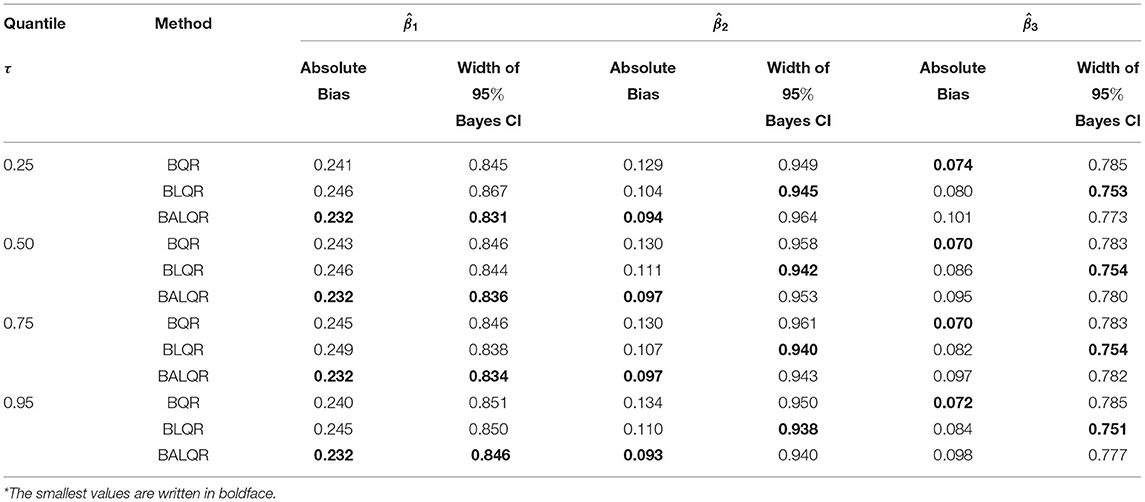
where each covariate x_ik is simulated from a standard normal distribution and β = (5, 1.5, 3). Three different distributions for e_i were considered: (i) heteroscedastic normal, (1 + x₁)N(0, 1), (ii) autocorrelated error, sin(seq(0.1π, 18.3π, 0.1π) + Z) with Z (0, 0.1), (iii) nonnormal error, the mixture of two Student's t distribution, 0.1t₍₁₎ + 0.9t₍₃₎. For each choice of the error distribution, we employed a Bootstrap resampling method with 100 simulations were carried out. In each simulation, 150 observations were generated. Four different values of the given quantile τ = 0.25, 0.50, 0.75, and 0.95 were considered. To assess the sampling efficiency of the proposed algorithm, the Monte Carlo standard errors for each β_k, k = 1, 2, 3 were calculated by running the Gibbs sampler for 5,000 iterations with an initial burn-in of 1,000 iterations to lessen the effect of initial simulations. The process resulted in 4,000 final posterior samples for each regression parameter. Then the width of 95% Bayes credible interval was estimated for each selected quantile for each proposed method. The absolute bias is also estimated when the estimates of ${\widehat{\beta }}_k$ were compared with the true value of β_k. The results are summarized in Tables 1–3.

TABLE 1

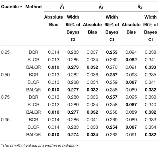
Table 1. The bias and width of 95% Bayes credible interval for heteroscedastic normal, e_i ~ (1 + x₁)N(0, 1)*.

Table 1 presents the results of all three proposed methods at several selected quantiles (i.e., τ = 0.25, τ = 0.50, τ = 0.75, and τ = 0.95). The table also presents the absolute bias and the width of 95% Bayes credible interval. The table shows that all proposed methods yielded very similar results. The table shows that, in general, Bayesian Adaptive Lasso quantile regression performs well compared to two other methods, BLQR and BQR.

Table 2 shows the results for autocorrelated errors. The table informs us that all proposed methods yielded almost similar values for corresponding quantiles. In general, BALQR performed best among the three methods because of the number of the smallest values of the entries.

TABLE 2

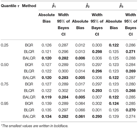
Table 2. The bias and width of 95% Bayes credible interval for autocorrelated error, e_i ~ sin(seq(0.1π, 18.3π, 0.1π)+Z_i) with Z ~ (0, 0.1)*.

Table 3 presents the absolute bias and the width of 95% Bayes credible interval for the three-parameter models of a nonnormal error condition. The results show that all values of the absolute Bias for corresponding quantiles are almost similar. Note that BALQR yielded the smallest values among the other three methods except for ${\widehat{\beta }}_3$. The Bayes credible intervals for all proposed methods at the same quantiles are almost similar. In general, the credible interval for BALQR is narrower than the other two methods.

TABLE 3

Table 3. The bias and width of 95% Bayes credible interval for non-normal, e_i ~ 0.1t₁ + 0.9t₃*.

The results concerning three different error distributions inform us of two things. First, although the performance of all the three methods proposed in this study is very close in general, the Bayes Adaptive Lasso quantile regression method performs better than the Bayes Lasso quantile regression and Bayes quantile method. Second, the BALQR method is robust to the error distribution assumptions, such as the normality assumption, the homogeneous assumption, or the non-correlated assumption. We assumed that the BALQR tends to produce more suitable values for the parameter estimated than other methods.

For the next analysis, we have to evaluate our algorithm's convergence used in the BALQR method. We use convergence diagnostics such as the posterior plots (trace plot and density plot) and autocorrelation analysis. Figures 1–3 present the trace plot, density plot, and autocorrelation plot of ${\widehat{\beta }}_1$ at quantile τ = 0.25 for all three conditions of error, i.e., heteroscedastic normal, autocorrelated error, and non-normal error, respectively. The author saves other plots for limited space.

FIGURE 1

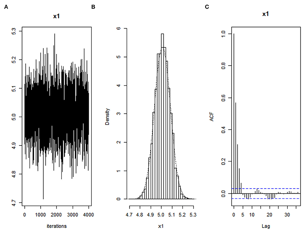
Figure 1. Convergence diagnostics of parameter ${\widehat{\beta }}_1$ for heteroscedasticity error when τ = 0.25 using Bayesian Adaptive Lasso quantile regression: (A) Trace plot, (B) density plot, and (C) autocorrelation plot.

As shown in the trace plots in Figures 1A, 2A, and 3A that all generated samples lie within two parallel horizontal lines, centered at respective values, and no trends are detected. The histograms of marginal posteriors in Figures 1B, 2B, and 3B above inform us that the conditional posterior distributions are the desired stationary univariate normal. All posterior distributions shrink at the true parameter value (trace plot and density plot). Furthermore, Figures 1C, 2C, and 3C inform that the decrease in the empirical autocorrelation of posterior samples proves that the underlying chains are stationary.

FIGURE 2

Figure 2. Convergence diagnostics of parameter ${\widehat{\beta }}_1$ for autocorrelated error when τ = 0.25 using Bayesian Adaptive Lasso quantile regression: (A) Trace plot, (B) density plot, and (C) autocorrelation plot.

FIGURE 3

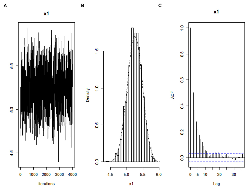
Figure 3. Convergence diagnostics of parameter ${\widehat{\beta }}_1$ for non-normal error when τ = 0.25 using Bayesian Adaptive Lasso quantile regression: (A) Trace plot, (B) density plot, and (C) autocorrelation plot.

The results obtained from these convergence diagnostics indicate that our algorithm used in the BALQR approach could produce adequate and acceptable values of the estimated parameter.

3.2. Modeling Low Birth Weight

3.2.1. Sample Data

The analysis is applied to the primary data related to Birth weight. The data was collected by distributing the online questionnaires from February to April 2020 to mothers who just delivered a singleton live birth and living in West Sumatera, Indonesia. In total, 150 respondents with complete information were involved in the analysis.

This study uses Birth weight, recorded in kilograms, as a response variable and 11 indicator variables, consisting of 6 variables in continuous type and five variables in categorical types. The continuous indicator variables were the Mother's age, Mother's weight gain (during pregnancy), Hemoglobin, Last birth interval, Parity, and Prenatal care. Meanwhile, the categorical indicator variables were Maternal education, Maternal occupation, Residence, Number of pregnancy problems, and Sex of the baby. Maternal education was divided into three levels; Low, Middle, and High level, where the Low level was set as a reference category, so coefficients were interpreted relative to this category. The Maternal occupation was classified into three categories, i.e., Government employee, Housewife, and Others. A Residence was categorized as Urban or Rural. Many pregnancy problems were categorized into three types: More than one problem, One problem, and No problem, where More than One problem was used as the reference category.

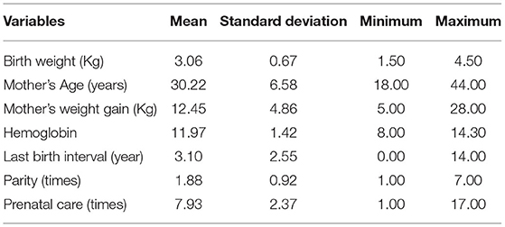
Table 4 displays the summary statistics for the continuous independents of the sample. The mean Birth weight data is 3.06, with the mean Mother's age being 30.22 years old. The average Mother's weight gain is 12.45 Kg and the mean of Hemoglobin is 11.97. On average, the mother's Last birth interval was 3.10 years ago. The mean of Parity is 1.88 times, and the mother had Prenatal care on average is 7.93 times.

TABLE 4

Table 4. Summary statistics for continuous independent variables of Birth Weight Data.

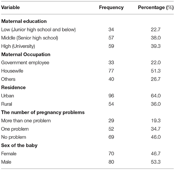
While Table 5 presents the summary statistics for categorical independents of the sample. In terms of Maternal educational attainment, 22.7% of mothers have a Low school education, 38% are Middle school, and 39.3 are University or College graduates. For the Maternal occupation variable, more than half of the mother's status is a Housewife (51.3%), 22.0% is a Government employee, and Others are 26.7%. More than half of mothers (64%) are living in urban areas. In terms of The number of pregnancy problems, most mothers have No problem while pregnancy (46%), 34.7% have One problem, and 19.3% have More than one problem. For the gender of babies, 46.7% are girls and 53.3% are boys.

TABLE 5

Table 5. Summary statistics of category independent variables.

3.2.2. Construction of LBW Model

In the preliminary analysis, we did several tests on the Birth weight model. Based on the test, it informs that the error of our model is violated by normality assumption and homoscedasticity. Then the quantile regression model between the response Birth weight and the eleven predictors without intercept was applied. In this empirical study, the frequentist quantile regression model is also employed for comparison purposes. The same equation shown in (1) is used here. The wild bootstrap method, as proposed by Feng et al. [38] and Yanuar and Zetra [39], was implemented for the quantile regression to get the parameter estimated. The procedures to use the wild bootstrap are as follows:

1. Fitting Equation (1) to the data to obtain the parameter vector of $\widehat{\beta }$ and the residual ê_i for i = 1, …, n.

2. Generate the weight w_i from an appropriate distribution and let $e_i^{*}=w_i\mid {ê}_i\mid$.

3. Calculate the bootstrap sample as $y_i^{*}=x_i^T\widehat{\beta }+e_i^{*}$.

4. Refit Equation (1) to the bootstrap sample and denote the bootstrap estimated by ${\widehat{\beta }}^{*}$.

5. Repeat Steps 2–4 until 100 times and estimate the mean and the variance of the 100 copies of ${\widehat{\beta }}^{*}$.

In constructing the proposed model, we did any model combination and compared it to obtain the best and most acceptable model, including allowing a model's simplicity (results for model comparison are available upon request).

Hence, our reduced model only involved the significant indicator variables, namely, Maternal education (consisting of 3 categories), The number of pregnancy problems (with three categories), and Parity. Thus, we consider the following quantile regression (QR) model:

$\begin{array}{l}Birthweigh{t}_i=\\ {\beta }_{1}Education{\left(Middle\right)}_i+{\beta }_{2}Education{\left(High\right)}_i+{\beta }_2\text{ Pro}blems\\ {\left(Oneproblem\right)}_i+\\ {\beta }_8\mathrm{Pr}oblems{\left(Noproblem\right)}_i+{\beta }_{9}Parit{y}_i+\epsilon i;\end{array}$

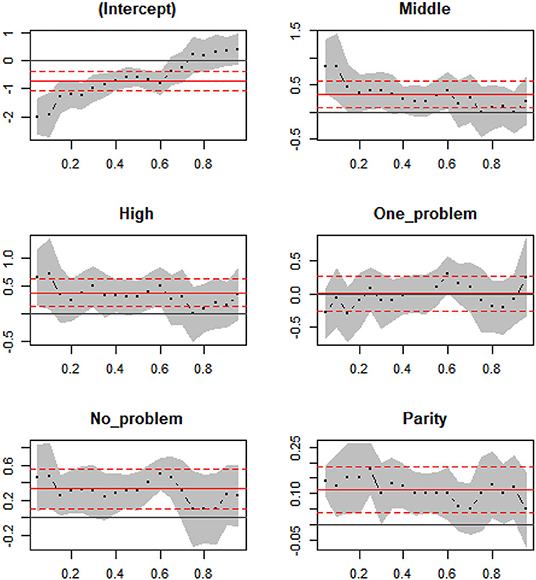
Figure 4 displays the quantile with CI estimated at any sequence quantiles shown with the grey area. The straight and dashed red line provides the OLS (Ordinary Least Square) estimated mean with its upper bound and lower bound for a 95% CI. This figure informs us that the width of 95% confidence interval based on OLS estimated seems to appear similar to quantiles, especially at lower quantiles.

FIGURE 4

Figure 4. Estimate coefficients for birth weight with 95% CI.

Table 6 summarizes the results for the estimated mean and the width of the 95% CI obtained based on quantile regression with the wild Bootstrap resampling method and modified quantile regression (BRQ, BLQR, and BALQR). Since LBW is focused on low quantiles, quantile t = 0.10, 0.25, and 0.50 were selected.

TABLE 6

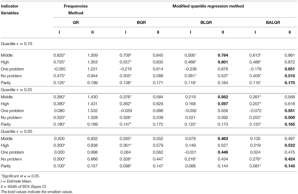
Table 6. The estimate mean and width of 95% Bayes credible interval for empirical data at quantile τ = 0.10, 0.25, and 0.50.

For the QR model at all selected quantiles τ, the 95% CI of the quantile is wider than each modified quantile method. These results have been predicted as the sample size is relatively small for the QR method (150 observations). Thus, in this analysis, QR does not produce an adequate model. ANOVA test also yielded that at selected quantile, the significant different due between quantile and respectively modified quantile. Furthermore, we could look at this table that at 0.10th quantile, all indicator variables for QR and modified QR are significantly difference from zero at the 5% level except for No problem. We also conclude here that BALQR tends to yield the shortest 95% CI among others.

The interpretation of the proposed model yielded based on BALQR is the 0.10th quantile (or percentile) of Birth weight for Middle is 0.613 Kg higher than Low, hold all else constant. The 0.10th quantile of Birth weight for High is 0.488 Kg higher than Low, assumed all else constant. Besides, the 0.10th quantile of Birth weight for No problem is 0.409 Kg higher than More than one problem. The impact of Parity on Birth weight is greater, for every increment of 1 unit of Parity, the Birth weight will increase by 0.116 Kg with assumptions else constant. A similar interpretation for model BALQR at 0.25th and 0.50th quantile could be created as well, except for No problem (not significant). While the 0.50th quantile for all four dummy variables is not significantly different from zero at the 5% level, only Parity. Parity, as a continuous variable, has a significant impact on Birth weight.

The next analysis is the convergency test for all estimated parameters. Figure 5 shows the diagnostic plots for Middle at the 0.25th quantile for illustrative purposes. The author saves other plots because of limited space.

FIGURE 5

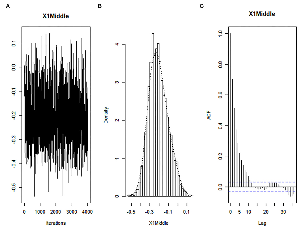
Figure 5. Convergence diagnostics of parameter ${\widehat{\beta }}_1$ (Middle) at τ = 0.25 using Bayesian Adaptive Lasso quantile regression: (A) Trace plot, (B) density plot, and (C) autocorrelation plot.

4. Conclusion

The study yields the acceptable model of LBW in West Sumatera, Indonesia, after doing a comparative study between three modification methods in quantile regression. The strength of the quantile method is that it can model the predictors' effects on the different quantiles of the response variable. It can accommodate non-normal errors since it is insensitive to heteroscedasticity and outliers. The quantile method's limitation requires a big sample size, and therefore, a quantile method should then be modified by combining it with the Bayesian approach. Under the Bayesian quantile regression approach, the parameter model is estimated by minimizing the check function, equivalent to maximizing a likelihood function formed by combining independently distributed asymmetric Laplace error distribution. This technique is robust to model small to moderate-sized samples and can handle any cases with violated normal assumptions. Generally, the Bayesian method needs no assumptions.

Even though many studies have been done on determining the LBW, no studies have been done on the modeling of the LBW model using a comparison of Bayesian quantile and its modification in this study. Not many studies have been done on constructing LBW using all 11 indicator variables as done in this present study. The indicators that are found significant in determining the LBW considered in this study are the mother's education at three levels: Middle, High, and Low level (as reference category), The number of pregnancy problems was categorized into three types: One problem, No problem, and More than one problem (as reference category), and Parity. These results are also linear with previous studies, such as research by Silvestrin et al. [5] and Yanuar et al. [18]. Here, the low birth weight model was constructed by involving 150 respondents. We assumed that these respondents were representing the condition of other mothers who just have a baby and living in West Sumatera. Based on data, we found that these size samples have met the requirement of sample adequacy. But, we argue to future research to use at least 200 samples to avoid misleading in such implementation of the quantile regression approach.

In this present study, we implemented the Wald method based on the asymptotic approximation to the variance-covariance matrix of the posterior sequences to estimate the Bayes credible interval. Based on simulation study and empirical study, it was proved that the Bayesian Adaptive Lasso quantile regression results in the smallest absolute Bias and the shortest 95% Bayes credible interval than the other two methods. This present study also gives a paramount significance to the attention of policymakers and decision-making organizations related to maternal pregnancy health to improve the adequacy of prenatal care use, facilitate the development of culturally sensitive interventions to enhance nutritional status and health of maternal pregnancy.

Data Availability Statement

The datasets presented in this article are not readily available because restrictions apply and are not publicly available. Requests to access the datasets should be directed to the corresponding author and with permission from West Sumatra Provincial Health Office, Indonesia.

Ethics Statement

The studies involving human participants were reviewed and approved by M. Djamil Hospital. Written informed consent to participate in this study was provided by the participants' legal guardian/next of kin.

Author Contributions

All authors listed have made a substantial, direct, and intellectual contribution to the work and approved it for publication.

Funding

This research was funded by Andalas University Research (PGB) Grant No.: T/3939/UN.16.17/PP.OK-KRPGB/LPPM/2019.

Conflict of Interest

The authors declare that the research was conducted in the absence of any commercial or financial relationships that could be construed as a potential conflict of interest.

Publisher's Note

All claims expressed in this article are solely those of the authors and do not necessarily represent those of their affiliated organizations, or those of the publisher, the editors and the reviewers. Any product that may be evaluated in this article, or claim that may be made by its manufacturer, is not guaranteed or endorsed by the publisher.

Acknowledgments

The authors are grateful to the editor and referee for their valuable suggestions and comments that greatly improved the manuscript.

References

1. Acharya D, Singh J, Kadel R, Yoo SJ, Park HJ, Lee K, et al. Maternal factors and utilization of the antenatal care services during pregnancy associated with low birth weight in rural Nepal: analyses of the antenatal care and birth weight records of the MATRI-SUMAN trial. Int J Environ Res Public Health. (2018) 15:2450. doi: 10.3390/ijerph15112450

PubMed Abstract | CrossRef Full Text | Google Scholar

2. Figueiredo A, Gomes-Filho I, Silva R, Pereira P, Mata F, Lyrio A, et al. Maternal anemia and low birth weight: a systematic review and meta-analysis. Nutrients. (2018) 10:601. doi: 10.3390/nu10050601

PubMed Abstract | CrossRef Full Text | Google Scholar

3. Lamichhane DK, Lee SY, Ahn K, Kim KW, Shin YH, Shu DI, et al. Quantile regression analysis of the socioeconomic inequalities in air pollution and birth weight. Environ Int. (2020) 142:105875. doi: 10.1016/j.envint.2020.105875

PubMed Abstract | CrossRef Full Text | Google Scholar

4. Spiegel E, Shoham-Vardi I, Sergienko R, Landau D, Sheiner E. The association between birth weight at term and long-term endocrine morbidity of the offspring. J Mater Fetal Neonatal Med. (2019) 32:2657–61. doi: 10.1080/14767058.2018.1443440

PubMed Abstract | CrossRef Full Text | Google Scholar

5. Silvestrin S, da Silva CH, Hirakata VN, Goldani AAS, Silveira PP, Goldani MZ. Maternal education level and low birth weight: a meta-analysis. J. Pediatr. (2013) 89:339–45. doi: 10.1016/j.jped.2013.01.003

PubMed Abstract | CrossRef Full Text | Google Scholar

6. Shi L, Macinko J, Starfield B, Xu J, Regan J, Politzer R, et al. Primary care, infant mortality, and low birth weight in the states of the USA. J Epidemiol Commun Health. (2004) 58:374–80. doi: 10.1136/jech.2003.013078

PubMed Abstract | CrossRef Full Text | Google Scholar

7. Yanuar F, Yozza H, Firdawati F, Rahmi I, Zetra A. Applying bootstrap quantile regression for the construction of a low birth weight model. Makara J Health Res. (2019) 23:90–5. doi: 10.7454/msk.v23i2.9886

CrossRef Full Text | Google Scholar

8. Soltani H, Lipoeto NI, Fair FJ, Kilner K, Yusrawati Y. Pre-pregnancy body mass index and gestational weight gain and their effects on pregnancy and birth outcomes: a cohort study in West Sumatra, Indonesia. BMC Womens Health. (2017) 17:102. doi: 10.1186/s12905-017-0455-2

PubMed Abstract | CrossRef Full Text | Google Scholar

9. Alhamzawi R, Yu K. Bayesian Lasso-mixed quantile regression. J Stat Comput Simulat. (2014) 84:868–80. doi: 10.1080/00949655.2012.731689

CrossRef Full Text | Google Scholar

10. Oh MS, Choi J, Park ES. Bayesian variable selection in quantile regression using the Savage “Dickey density ratio. J Kor Stat Soc. (2016) 45:466–76. doi: 10.1016/j.jkss.2016.01.006

CrossRef Full Text | Google Scholar

11. Saputri OD, Yanuar F, Devianto D. Simulation study the implementation of quantile bootstrap method on autocorrelated error. Cauchy. (2018) 5:95–101. doi: 10.18860/ca.v5i3.5349

CrossRef Full Text | Google Scholar

12. Zhen Z, Cao Q, Shao L, Zhang L. Global and geographically weighted quantile regression for modeling the incident rate of children's lead poisoning in Syracuse, NY, USA. Int J Environ Res Public Health. (2018) 15:2300. doi: 10.3390/ijerph15102300

PubMed Abstract | CrossRef Full Text | Google Scholar

13. Peters G. General quantile time series regressions for applications in population demographics. Risks. (2018) 6:97. doi: 10.3390/risks6030097

CrossRef Full Text | Google Scholar

14. Sigauke C, Nemukula M, Maposa D. Probabilistic hourly load forecasting using additive quantile regression models. Energies. (2018) 11:2208. doi: 10.3390/en11092208

CrossRef Full Text | Google Scholar

15. Tu S, Wang M, Sun X. Bayesian variable selection and estimation in maximum entropy quantile regression. J Appl Stat. (2017) 44:253–69. doi: 10.1080/02664763.2016.1168369

CrossRef Full Text | Google Scholar

16. Oh MS, Park ES, So BS. Bayesian variable selection in binary quantile regression. Stat Probabil Lett. (2016) 118:177–81. doi: 10.1016/j.spl.2016.07.001

CrossRef Full Text | Google Scholar

17. Yanuar F, Ibrahim K, Jemain AA. Bayesian structural equation modeling for the health index. J Appl Stat. (2013) 40:1254–9. doi: 10.1080/02664763.2013.785491

CrossRef Full Text | Google Scholar

18. Yanuar F, Zetra A, Muharisa C, Devianto D, Putri AR, Asdi Y. Bayesian quantile regression method to construct the low birth weight model. J Phys. (2019) 1245:012044. doi: 10.1088/1742-6596/1245/1/012044

CrossRef Full Text | Google Scholar

19. Li Q, Xi R, Lin N. Bayesian regularized quantile regression. Bayesian Anal. (2010) 5:533–56. doi: 10.1214/10-BA521

CrossRef Full Text | Google Scholar

20. Alhamzawi R, Yu K. Variable selection in quantile regression via Gibbs sampling. J Appl Stat. (2012) 39:799–813. doi: 10.1080/02664763.2011.620082

PubMed Abstract | CrossRef Full Text | Google Scholar

21. Ji Y, Lin N, Zhang B. Model selection in binary and tobit quantile regression using the Gibbs sampler. Comput Stat Data Anal. (2012) 56:827–39. doi: 10.1016/j.csda.2011.10.003

CrossRef Full Text | Google Scholar

22. Chen CWS, Dunson DB, Reed C, Yu K. Bayesian variable selection in quantile regression. Stat Its Interface. (2013) 6:261–74. doi: 10.4310/SII.2013.v6.n2.a9

CrossRef Full Text | Google Scholar

23. Benoit DF, Alhamzawi R, Yu K. Bayesian lasso binary quantile regression. Computat Stat. (2013) 28:2861–73. doi: 10.1007/s00180-013-0439-0

PubMed Abstract | CrossRef Full Text | Google Scholar

24. Muharisa C, Yanuar F, Devianto D. Simulation study the using of Bayesian quantile regression in nonnormal error. Cauchy. (2018) 5:121–6. doi: 10.18860/ca.v5i3.5633

CrossRef Full Text | Google Scholar

25. Yanuar F, Yozza H, Zetra A. Bayesian quantile regression methods in handling non-normal and heterogeneous error term. Asian J Scientific Res. (2019) 12:346–51. doi: 10.3923/ajsr.2019.346.351

CrossRef Full Text | Google Scholar

26. Benoit DF, Van den Poel D. Binary quantile regression: a Bayesian approach based on the asymmetric Laplace distribution. J Appl Econometr. (2012) 27:1174–88. doi: 10.1002/jae.1216

CrossRef Full Text | Google Scholar

27. Yu K, Moyeed RA. Bayesian quantile regression. Stat Probabil Lett. (2001) 54:437–47. doi: 10.1016/S0167-7152(01)00124-9

CrossRef Full Text | Google Scholar

28. Feng Y, Chen Y, He X. Bayesian quantile regression with approximate likelihood. Bernoulli. (2015) 21:832–50. doi: 10.3150/13-BEJ589

CrossRef Full Text | Google Scholar

29. Alhamzawi R, Yu K, Benoit DF. Bayesian adaptive Lasso quantile regression. Stat Model. (2012) 12:279–97. doi: 10.1177/1471082X1101200304

CrossRef Full Text | Google Scholar

30. Choi HM, Hobert JP. Analysis of MCMC algorithms for Bayesian linear regression with Laplace errors. J Mult Anal. (2013) 117:32–40. doi: 10.1016/j.jmva.2013.02.004

CrossRef Full Text | Google Scholar

31. Kozumi H, Kobayashi G. Gibbs sampling methods for Bayesian quantile regression. J Stat Comput Simulat. (2011) 81:1565–78. doi: 10.1080/00949655.2010.496117

PubMed Abstract | CrossRef Full Text | Google Scholar

32. Zou H. The adaptive lasso and its oracle properties. J Am Stat Assoc. (2006) 101:1418–29. doi: 10.1198/016214506000000735

CrossRef Full Text | Google Scholar

33. Andrews DF, Mallows CL. Scale mixtures of normal distributions. J R Stat Soc B. (1974) 36:99–102. doi: 10.1111/j.2517-6161.1974.tb00989.x

CrossRef Full Text | Google Scholar

34. Xu D, Tang N. Bayesian adaptive Lasso for quantile regression models with nonignorably missing response data. Commun Stat Simulat Comput. (2019) 48:2727–42. doi: 10.1080/03610918.2018.1468452

CrossRef Full Text | Google Scholar

35. Yang Y, Wang HJ, He X. Posterior inference in bayesian quantile regression with asymmetric laplace likelihood: bayesian quantile regression. Int Stat Rev. (2015) 84:327–44. doi: 10.1111/insr.12114

PubMed Abstract | CrossRef Full Text | Google Scholar

36. Yue YR, Hong HG. Bayesian Tobit quantile regression model for medical expenditure panel survey data. Stat Model. Int. J. (2012) 12:323–46. doi: 10.1177/1471082X1201200402

CrossRef Full Text | Google Scholar

37. Alhamzawi R, Ali HTM. Brq: an R package for Bayesian quantile regression. Metron. (2020) 78:313–28. doi: 10.1007/s40300-020-00190-6

CrossRef Full Text | Google Scholar

38. Feng X, He X, Hu J. Wild bootstrap for quantile regression. Biometrika. (2011) 98:995–9. doi: 10.1093/biomet/asr052

PubMed Abstract | CrossRef Full Text | Google Scholar

39. Yanuar F, Zetra A. Length-of-stay of hospitalized COVID-19 patients using bootstrap quantile regression. IAENG Int J Appl Math. (2021) 51:1–12. Available online at: http://www.iaeng.org/IJAM/issues_v51/issue_3/IJAM_51_3_40.pdf