Self-Retrospect Periphery Gate Model and Its Applications

By not only relying on the initial state but also relying on states before, the principle of a self-retrospect dynamic system has been developed to represent the changes in a system since 1991. Afterward, the periphery theory was established, which studies the boundary of a system. We try to integrate the principle of the self-retrospect system and periphery theory in this study. Thus, a self-retrospect periphery gate model, a new expression of temporal-spatial concept, has been derived to investigate the change of a system and forecast it in physics. Firstly, for the equation with a time difference term that controls the motion of the system, a difference-integral equation can be derived by introducing a retrospect function and applying the inner product, partial integral, and mean value theorem. The principle of constructing and solving the difference-integral equation of the system is referred to as the principle of self-retrospect dynamic systems, and the corresponding mathematical model is called the self-retrospect model. The principle of system self-retrospect has been applied to modeling, calculating, and forecasting in many fields such as meteorology, oceanography, hydrology, market, agriculture, transportation, energy, and so on. Secondly, the periphery is defined as an intermediary that can protect the system and exchange with the environment. It is a part of the system and is adjacent to the environment. It has been applied in many fields since the periphery theory was put forward, such as physics, meteorology, water resources, economy, as well as sports. Thirdly, the concept of periphery gate is embedded into the self-retrospect equation, the self-retrospect gate model has been proposed, and the physical implication of the model is mentioned. The mathematical derivation of the model and its physical explanation are the main points of the study. The applications of the model in physics and meteorology are discussed, for example, the relationship between heavy snowfall and airflow passage in Beijing was studied using synoptic meteorology in detail.

Introduction

The quantitative study of system memory can be carried out using Langevin Equation, delay differential equation, difference-integral equation, and so on. In time series analysis, the stochastic differential equation is usually employed to describe the relationship between the system states at different times, and it is another way of quantitatively studying the system memory.

The future change of a system is not only related to its present state but also related to its past state. Markov process is only an abstraction and simplification. In fact, the change of a system is always related to its history, or a system will always remember its past, although the “memory” or forgetting factor is different for various systems. For example, due to the nature of the fluid, the memory of the ocean is stronger than that of the atmosphere. Compared with the movement of the atmosphere, the ocean moves slower. Therefore, the information about the past state of atmosphere may still exist in the current state of the ocean. Thus, we should study not only the self-retrospect system but also the correlation between different systems. The study of system memory is not only an abstraction in respect of theory but also has an experimental basis. For example, the memory of Brownian motion was confirmed by experiments, and memory exists in ion passages of biofilm. Since the principle of self-retrospect dynamic system was put forward in 1991, it has been applied to many fields, such as meteorology, oceanography, hydrology, market, agriculture, transportation, and energy [1, 2]. For example, it can be used for forecasting and improving forecasting accuracy significantly [3–7].

By introducing a retrospect function and applying the inner product, partial integration, and mean value theorem to the equations containing time difference terms, a difference-integral equation can be derived, which contains both multiple past values and initial values. Solving the difference-integral equation constitutes a new forecast and calculation technique. The principle of constructing and solving the difference-integral equation of the system is also called the principle of self-retrospect of the system. The mathematical model derived from the principle is referred to as a self-retrospect model. The principle of self-retrospect emphasizes the continuity and evolution of the system state. At this point, a unique concept and mathematical method have been developed. The principle of system self-retrospect has been successfully applied in many fields, especially in weather forecast and climate prediction. Combined with the numerical model to solve the initial and boundary value problems of differential equations, and by means of a statistical model based on observation data, self-retrospect model not only has distinct originality in academic but also is very useful in practice. Based on the idea of using multi-time measurements, a new backtracking difference scheme is proposed, which significantly improves the calculation accuracy compared with traditional difference schemes.

There are a lot of periphery phenomena in both the material world and spiritual world, such as the eyewall of a hurricane [8–10], the shell of eggs, the earth's atmosphere [11], people's clothes, biofilm, national boundaries, underworld organizations, and so on. One example is the border between two countries, where only customs allow goods and personnel to enter and leave. In fact, how many goods and people pass through customs reflects whether a country or region is a developed or a developing country or region. The European castles and the Great Wall of China were used to defend against the alien invasion, but their gates are used as passages for the exchange of goods and people. A house was built to withstand wind, rain, and wild animals, while the narrow door allows people and materials to enter and leave (Figure 1).

FIGURE 1

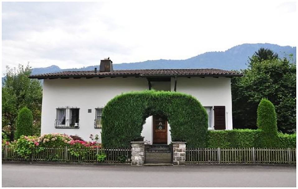
Figure 1. House.

The periphery theory is a general theory to study system periphery, that is, to study some common laws of system periphery and their applications in the fields of information theory, cybernetics, environment, physics, biology, management, decision-making, psychology, aesthetics, philosophy, etc. [12–14]. Its basic academic idea is that the input and output of energy, material, and information of a real system through the periphery gate must be controlled by the periphery. In another word, the state of a system and its periphery mutually govern each other. The problems in different fields such as system balance, life existence, and ethnic conflict are discussed from different points of view.

The purpose of periphery theory is to study the periphery shell focusing on the following features: (1) the survival and development of the system; (2) the exchange between the system and its surrounding environment. To exchange with the environment, there must be periphery gates on the periphery, that is, there must be passages through which the energy, material, and information can pass. The number of passages determines the occurrence and development of a system.

Based on the self-retrospect principle of dynamic system and periphery theory, a self-retrospect periphery gate model is proposed by combining the two. The main purpose of this study is to mathematically derive the self-retrospect periphery gate model and to explain the physical implications. Beyond that, the possible applications of the model in some fields are discussed, particularly the relationship between the heavy snow and the airflow passages around Beijing.

Study Methods

Self-Retrospect Principle

Without losing generality, the differential equation of system evolution can be written as

$\begin{array}{ll}\frac{\partial x}{\partial t}=F(x,\lambda ,r,t)& (1)\end{array}$

where x is a variable, λ is a parameter, r is space, and t is time. Equation (1) indicates the relationship between the local time variation of x and the source function (or field function, also known as the space term). F can include differential, difference, integral, or other functions. The retrospect function β(r, t) is a function of r and t, and |β(r, t)|≤1. Inner product in Hilbert space is given by:

$\begin{array}{ll}(f,g)=\int f(\zeta )g(\zeta )d(\zeta )f,g\in L^2& (2)\end{array}$

We use this inner product to transform Eq. (1), assuming that the variables x and ß are continuous, differentiable, and integrable, and a difference integral equation can be derived by using the partial integral and mean value theorem in calculus [12].

$\begin{array}{l}\beta (r,t)x(t)=\beta (r,t_{-p})x(t_{-p})+\\ {\displaystyle \sum _{i=-p}^0(\beta (r,t_{i+1})-\beta (r,t_i))x^m(t_i)+{\displaystyle {\int }_{i_{-p}}^i\beta (r,t)F(x,\lambda ,r,t)d_t}}& (3)\end{array}$

where t₀ is the time, p is the retrospective order, that is, the number of variables and state fields before t₀, $x^m(t_i)$ is the median between t_i and t_i+1, namely $x^m(t_i)\equiv x(t_m),t_i<t_m<t_{i+1}$. If x(t) is regarded as the forecast time, then the second and third terms in (2) represent the contribution of the local past value of p + 1 time to x(t), which is called the self-retrospect term. The fourth term is the contribution of p + 1 state field F(x, λ, r, t) to x(t), which is called the other effect item. Formula (2) emphasizes the relationship between the preceding system state and the subsequent system state, that is, the memory of the system itself, so formula (2) is called the self-retrospect equation of the system.

Once the retrospect function β is determined by historical measurement data, formula (2) can be used for simulation or prediction. The model based on the difference integral Equation (2) is called the self-retrospect model, and F(x, λ, r, t) in (2) is called the dynamic kernel. The principle of transforming a differential equation into a difference integral equation by introducing the retrospect function and solving it is called the self-retrospect principle.

The equal interval sampling is taken as Δt, that is, t_i = t₀ + iΔt, i = 1, 0, −1, −2,, −p, t₀ is the initial time, t = t₀ + Δt is a one-step prediction, and p the is retrospective order.

When the mean value is equal to the average of the two times before and after, the integral is replaced by summation and the expression (2) becomes discretization, abbreviated as R, and the expression (2) can be changed into

$\begin{array}{ll}x(t)={\displaystyle \sum _{i=-p}^0}{\alpha }_{i}x(t_0+i\Delta t)+{\displaystyle \sum _{i=-p}^0}{\theta }_i(r)F(x,\lambda ,t_0+i\Delta t)\Delta t& (4)\end{array}$

where α_i and θ_i are memory coefficients, which are composed of retrospect functions, reflecting the memory degree of the system at different past times, that is, the weight of contribution to x(t) at different times in mathematics. When there are historical observation data, α_i and θ_i can be determined by the least square, genetic algorithm, and artificial neural network. Once the memory coefficient is determined, the system can be simulated or predicted by formula (3).

Formula (2) is the basic equation of the self-retrospect model, which is obviously different from other existing methods to quantitatively study system memory. It uses a retrospect function to investigate the influence of different times and different factors on the future system state. When comparing formula (2) with formula (1), there is an extra retrospect function β(r, t) and retrospective order p needs to be determined. Therefore, solving formula (2) is more complex than solving formula (1), and usually it can only be solved numerically.

The retrospect function β(r, t) and retrospective order p are included in formula (2), which increases the plasticity of Equation (2), that is, by determining β(r, t) and p, Equation (2) is more suitable for the problem itself, and then the determination of β(r, t) and p becomes an optimization problem. The solution to Equation (1) is formula (4):

$\begin{array}{ll}\begin{array}{c}x(t)=x(t_0)+{\displaystyle {\int }_{t_0}^{t}F(\tau )d_{\tau }}\end{array}& (5)\end{array}$

Obviously, the numerical solution of difference integral Equation (2) is quite different from that of differential Equation (1).

An interesting mathematical problem is that many different schemes in numerical calculation can be deduced from the difference integral Equation (3) with a certain value provided by the retrospect function. According to this, the relationship [2] between Equation (3) and various calculation schemes of Equation (4) can be concluded. From these analyses, we can see the generalized properties of the difference integral equation. For differential equations with analytic solutions

$\begin{array}{ll}\frac{d_x}{d_t}=-x+2cost& (6)\end{array}$

The second-order difference quotient method and the self-remembering backtracking scheme are used for numerical integration, respectively [15, 16]. The results show that the accuracy of the latter is 10⁻⁷ and that of the former is 10⁻⁴. A so-called gray model GM (1,1) is applied to solve the equation [17]. The accuracy of absolute value error is 10⁻² and increases rapidly, while the accuracy of the self-recalling backtracking scheme is less than 10⁻⁶.

The differential equation can be derived by inversion for a system without differential equation description with a certain sampling length, and then the principle of self-retrospect is applied to the equation, thus a new way of dynamic data modeling is developed [18, 19].

The advection equations in fluid mechanics are calculated by using the backtracking scheme and frog leaping scheme, respectively, with the ideal field as the initial field and the flow field. The results show that the accuracy of the former is 2 to 5 times higher than that of the latter [2].

Self-Retrospect Periphery Gate Model

In the differential equations describing diffusion, heat conduction, convection, and other phenomena, the difference term of physical quantity to space is included, so the retrospect function is naturally related to space r. When the retrospect function is not only a function of time but also an explicit function of space, formula (2) can be transformed into a self-retrospect periphery gate model. In other words, the idea of periphery gate is introduced into the self-retrospect equation to combine the self-retrospect principle of the dynamic system with the theory of periphery shell. In ocean dynamics, the Strait is a periphery gate. In meteorology, both canyon and mountain pass play the role of periphery gate. Due to the human intervention in nature, such as building dams on rivers and setting checkpoints on roads, it has become a problem that could be described by the self-retrospect periphery gate model. The model can be applied to dynamic problems such as traffic flow, hydrology, cell membrane, and military models.

Let θ_i(r) be a separable multiplicative model of time and space, then θ_i(r) = θ_rθ_i

then Equation (3) becomes

$\begin{array}{ll}x(t)={\displaystyle \sum _{i=-p}^0}{\alpha }_{i}x(t_0+i\Delta t)+{\theta }_r{\displaystyle \sum _{i=-p}^0}{\theta }_{i}F(x,\lambda ,t_0+i\Delta t)\Delta t& (7)\end{array}$

when θ_r is a switch type, that is, θ_r ∈ {0, 1}, it acts as a periphery gate. When θ_r ∈ [0, 1], it acts as a fuzzy periphery gate.

The self-retrospect periphery gate model elucidates the view of time and space from a new perspective. The system is non-uniform in time, which is reflected in the change of memory coefficient with time, or the change of forgetting factor of the complement of memory coefficient. The retrospective order defined as p is the assumption that the system state before p has no influence on the future. If we assume that the retrospect function decays exponentially with time, then only when p → ∞, and it has no effect on the future of the system, and only by truncation can we determine the limited retrospective order. In other words, the development direction of the system is determined by the memory characteristic of the system in the time direction. The existence of the periphery gate changes the spatial configuration on both sides of the system and even leads to the opposite spatial distribution, which leads to the breaking of spatial symmetry. The passing of time is not governed by any periphery wall or gate, but its memory affects the development and change of the system, that is, the past and the present determine the future. Speaking of space, there are many kinds of periphery everywhere, as a metaphor, there are “fences” everywhere in the space. Only the periphery door can allow the flow of material, energy, and information. In other words, time and space are totally different philosophically [20]. The self-retrospect periphery gate equation is the expression of this philosophy, which is different from the space-time view derived from the second law of thermodynamics [21–23]. It should be said that the potential scientific significance of the self-retrospect periphery gate model is very profound.

Applications

In the Yangtze River Basin, there are three famous hot-summer cities, namely Chongqing, Wuhan, and Nanjing, and they are called the “three furnaces” in China. In fact, they are all related to their special topography, land-surface, and vegetation. The self-retrospect periphery gate model can be employed to simulate the flow field of these cities and their surrounding areas, identify some sensitive terrain points, and change the flow field by opening ventilation tunnels or man-made canyons to achieve the purpose of cooling. This is potentially doable in the near future.

The atmospheric barotropic model is a classical model of weather forecast [18, 24]. A self-retrospect backtracking scheme is formulated on basis of the principle of self-retrospect. The backtracking scheme and central difference scheme are used to calculate the barotropic model, respectively. Subsequently, the calculated value is compared with the Hurwitz wave function solution of the model. The results show that the accuracy of the former is 1 to 2 orders of magnitude higher than that of the latter [25].

The self-retrospect periphery gate model can also be used in hydrological calculation. For instance, the water discharge of the Yangtze River at Wuhan is related to the state of the Three Gorges Dam, whether it is releasing water or not, what date/season it releases water, and how long it releases water.

Lu et al. [15] applied the principle of self-retrospect to the calculation of cross-section discharge in hydrology and calculated the discharge with Muskingen method and self-retrospect model, respectively. Both methods can calculate the downstream discharge fairly well, but the self-retrospect model method has a higher accuracy than the Muskingen method. The relative error of self-retrospect periphery model is 1.6%, while that of the Muskingen method is 3.5%. The accuracy is improved by (3.5–1.6) / 3.5 = 54%. Due to the high accuracy of Muskingen method, the improvement is not easy, which shows the strong ability of self-retrospect model to improve the prediction.

In the past, we have discussed the relationship between artificial neural networks and the self-retrospect model. Network memory, network channel, and other issues need to be addressed in the network environment of intelligent computing problems. Self-retrospect periphery gate model is suitable to complement both of them.

Case Study

Weather Overview

On 5 January, 2020, it began to snow in Beijing toward evening, and gradually became steady at night. By 6:00 the next morning, the snowfall in many places had reached the level of moderate or heavy level. Especially, some areas in the northwest even reached the category of a blizzard. At 14: 00 on 6th January, the average snowfall in Beijing was 3.1 mm, and that in urban areas was 4.9 mm. The heaviest snowfall occurred in Erhaituo, Yanqing District, reaching 10.4 mm. This is the third-heaviest blizzard in Beijing since November 2019. Finally, this snow in the Beijing plain generally reached a thickness of 5–7 cm.

Circulation Situation

The 500 hPa circulation at 08:00 on 5th January showed (Figure 2) that there was a −32°C cold center in Siberia, and the Lake Baikal trough merged with the small trough in Qinghai and moved eastward and formed the north branch of the westerly trough from Lake Baikal to Alexa. There was a south branch trough in the Bay of Bengal, and the front of it cooperated with the warm ridge and pushed the southwesterly warm and humid airflow northward over to Beijing. The depression of the dew point t-t_d in Beijing was <4°C, and the humidity was obviously increasing. At 20:00 on 5th January (Figure 3), the north-westerly trough moved into the Hetao area, and Beijing was located in the southwest airflow passage in front of the trough. Due to the combination of cold airflow and warm airflow, the temperature dew-point difference was t-$t_d\le 1^{°}$C, and snowfall occurred in Beijing. At 08:00 on 6th June, the south branch trough moved to the east of Qinghai–Tibet Plateau, and the southwest airflow in front of the trough developed vigorously. The north-westerly trough was located in the northern part of North China. This trough moved eastward and carried weak cold air southward, which provided a weak cold air condition for the snowfall in Beijing.

FIGURE 2

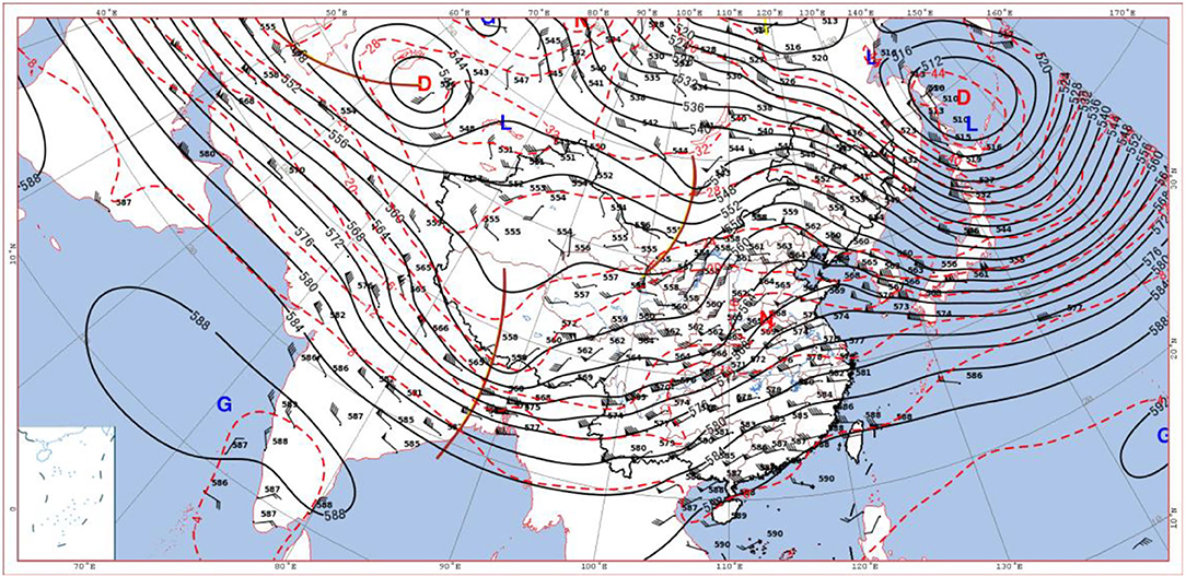
Figure 2. Wind field, height field (black isolines), and temperature field (red isolines) at 500 hPa at 08:00 on 5 January 2020 (G, D, N, and L are high-pressure center, low-pressure center, warm center, and cold center in turn, respectively).

FIGURE 3

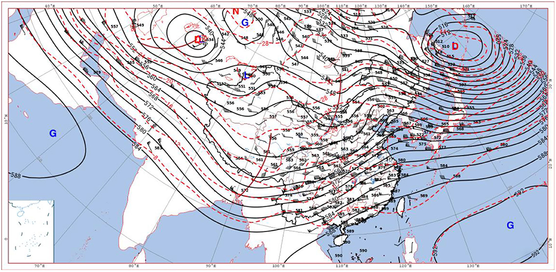
Figure 3. Wind field, height field (black isolines), and temperature field (red isolines) at 500 hPa at 20:00 on 5 January 2020 (G, D, N, and L are high-pressure center, low-pressure center, warm center, and cold center in turn, respectively).

The situation at 700 hPa was similar to that of 500 hPa: the warm air was observed to be strong in the early stage (Figure 4), while there was a cold vortex in the northeast of Japan and the west coast of the Pacific Ocean. Moreover, behind the cold vortex, there was ahigh-pressure ridge from the South China Sea to Hulunbuir area. The north-westerly trough was formed from Lake Baikal to Alexa, and the temperature trough lagged behind the height trough, which contributed to the deepening of the trough. At 20:00 on 5th January (Figure 5), the cold shear crossed Beijing with the eastward movement of the system. Meanwhile, the northwestern cold air behind the shear met the southwestern warm and humid air in the front of the shear and the warm and the humid airflow carried by the southwest gale belt, all these contributed much to the formation of the convection. In addition, t-t_d was <1°C. Under the combined influence of sufficient southwest water vapor supplement, the northwest cold air in front of cold high pressure and shear, and the three airflow passages around Beijing led to the large-scale snowfall in January 2020.

FIGURE 4

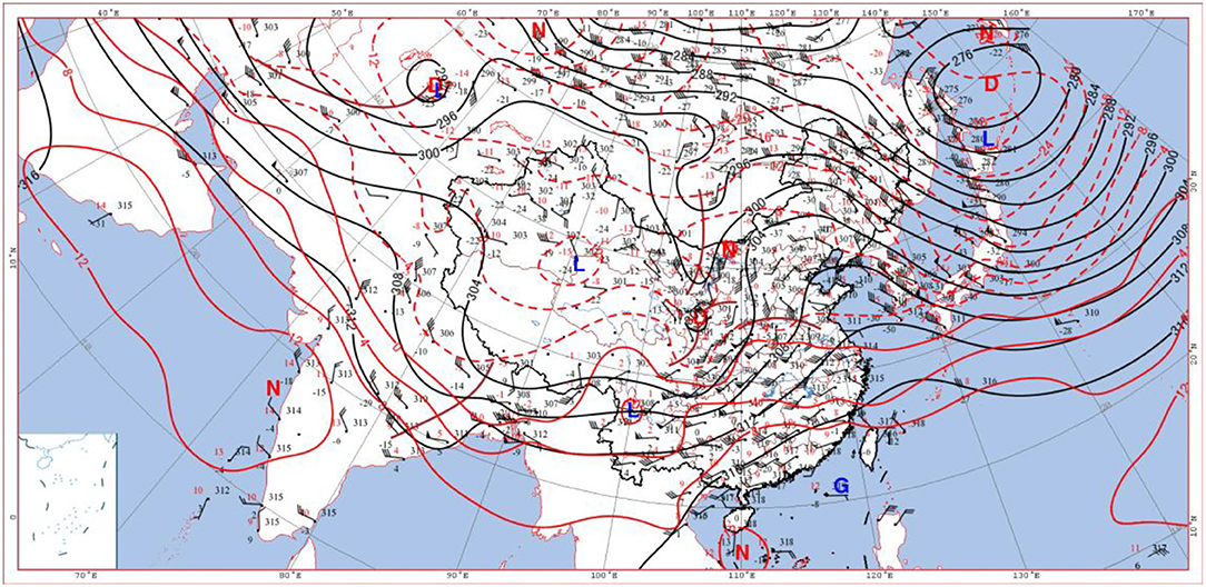
Figure 4. Wind field, height field (blue isolines), and temperature field (red isolines) at 700 hPa at 08:00 on 5 January 2020 (G, D, N, and L are high-pressure center, low-pressure center, warm center, and cold center in turn, respectively).

FIGURE 5

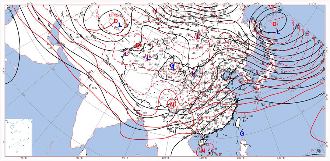
Figure 5. Wind field, height field (black isolines), and temperature field (red isolines) at 700 hPa at 20:00 on 5 January 2020 (G, D, N, and L are high-pressure center, low-pressure center, warm center, and cold center in turn, respectively).

At 08:00 on 5th January, there was a southwest vortex of 850 hPa in the lower level in Sichuan (Figure 6), and its front transverse trough guided the southeast warm and humid airflow northward, which was more obvious than the upper-level warm advection, resulting in unstable air stratification with upper cold and lower warm. There was a cold high-pressure center in the west of Lake Baikal, which pushed the cold air eastward and southward, deepening the development of its front trough. The southeasterly airflow with a wind speed of 10–12 m·s⁻¹ on the north side of the warm shear line between the Yangtze River and the Huaihe River transported water vapor from the east sea to Beijing. At 20:00 of 5 May (Figure 7), Beijing was in a trough of low pressure between the two highs. At the same time, the southern part of Beijing was affected by the warm and humid shear, and a closed low-pressure system was formed near the Sichuan Basin. The southerly airflow in front of it carried abundant water vapor northward to Beijing, and the wet area with $t-t_d\le 1^{°}$C had begun to affect Beijing, and sufficient water vapor led to a large-scale snowfall in Beijing. In the afternoon of 6 June, the snowfall ended as the cold high pressure gradually controlled this area.

FIGURE 6

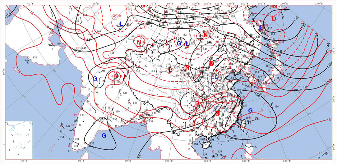
Figure 6. Wind field, height field (black isolines), and temperature field (red isolines) at 850 hPa at 08:00 on 5 January 2020 (G, D, N, and L are high-pressure center, low-pressure center, warm center, and cold center in turn, respectively).

FIGURE 7

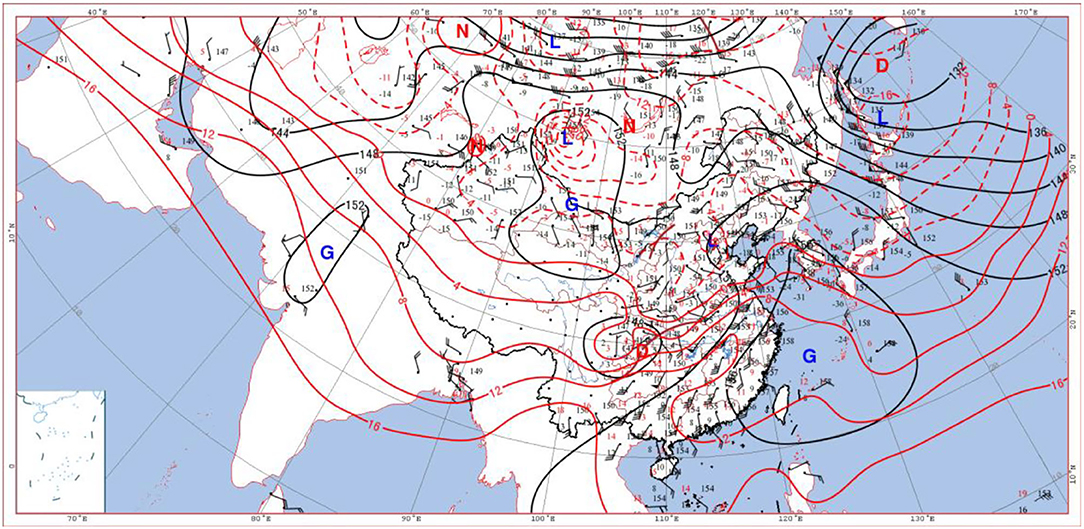
Figure 7. Wind field, height field (black isolines), and temperature field (red isolines) at 850 hPa at 20:00 on 5 January 2020 (G, D, N, and L are high-pressure center, low-pressure center, warm center, and cold center in turn, respectively).

In summary, the airflow passages at 500, 700, and 850 hPa clearly indicated that the upper atmosphere above 500 hPa was controlled by the warm and humid southwesterly airflow (purple arrow); and the wide southwesterly airflow transported the warm and humid air from the Bay of Bengal and the South China Sea to Beijing. Both warm and humid airflows met the southward cold air guided by the unstable trough in the north, which resulted in heavy snowfall in Beijing. The middle atmosphere of 700 hPa was dominated by southerly warm and humid airflow (brown arrow), and abundant water vapor was transported toward the north and converged in North China. Its upward movement made the precipitation develop and reached the strongest stage rapidly. There was a strong southeast wind (red arrow) at and below 850 hPa (Figure 8). The three airflow passages cooperated with each other and continuously transported abundant water vapor from the South China Sea, the East China Sea, and the Yellow Sea to Beijing, and provided a favorable large-scale circulation field for the occurrence of heavy snowfall, finally resulting in / heavy snowstorms in Beijing. A careful survey of the areas surrounding Beijing at 850 hPa reveals that there were several northeast-southwest wind directions on the northeast edge of Beijing, which would lead to the easterly airflow on the ground and form the turbulent weather finally. The turbulent weather was necessary for heavy snowfalls in Beijing. The heavy snow weather was the result of the intersection of the three airflows from different passages. This is an example of the application of the multi-passage in periphery theory to weather analysis.

FIGURE 8

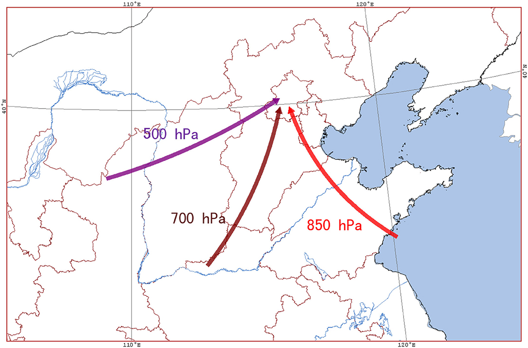
Figure 8. Integration of three air flow passages of 500, 700, and 850 hPa.

The research results by Jiang et al. [26], Zhang et al. [27], Guo [28], and Su and Zheng [29] also support this conclusion.

Conclusions and Discussion

Based on the principle of self-retrospect of dynamical system and periphery theory, the self-retrospect periphery gate model is established and discussed in this study.

The principle of self-retrospect of system emphasizes the continuous relationship between the system state and its evolution law; thus a unique concept and mathematical method has been developed. The principle of self-retrospect of system combines the numerical model, which solves the initial value and boundary problems of differential equations, with the statistical model based on observation data.

The self-retrospect model not only has distinct academic originality but also is very useful in practice. Based on the idea of using multi-time measurements, a new difference and back-tracking scheme has been proposed, which significantly improved the calculation accuracy compared with traditional difference schemes. For example, it has higher accuracy than the Muskingen method [15] does. It widened the application range of GM (1, 1) model and overcome the limitation of “sensitive to initial value,” which comes with GM (1, 1) model by using only one initial value for forecasting. These are of great significance to improve forecasting and calculation in many fields of science and technology.

The theory of periphery discusses the problems in different disciplines such as system balance and life existence from a new point of view. It is beneficial to inspire people to study natural sciences and social sciences further. From the perspective of the periphery theory, people can rethink the existing concepts and theories, including artificial intelligence.

The self-retrospect periphery gate model is an organic combination of self-retrospect principle with periphery theory. It is a philosophical expression of space-time view, which is different from the space-time view derived from the second law of thermodynamics. The self-retrospect periphery gate model is of latent scientific significance, which broadens our horizons of dynamic modeling.

This study analyzed a snowfall in Beijing in detail, studied its relationship with the multi-passage airflows of Beijing, and illustrated the applicability of the self-retrospect periphery gate model in weather forecasting.

Data Availability Statement

The original contributions presented in the study are included in the article/supplementary files, further inquiries can be directed to the corresponding author.

Author Contributions

XC, HC, and XF: conceptualization, methodology, formal analysis, investigation, and writing-original draft preparation. CC, WF, and YY: investigation. XC, HC, XF, and JS: revision. JS, CC, WF, and YY: proofreading and editing. All the authors have read and agreed with the published version of this paper. All authors contributed to the article and approved the submitted version.

Funding

This research is funded by the Basic Research Fund (2021Z001) of Chinese Academy Meteorological Sciences.

Conflict of Interest

The authors declare that the research was conducted in the absence of any commercial or financial relationships that could be construed as a potential conflict of interest.

Publisher's Note

All claims expressed in this article are solely those of the authors and do not necessarily represent those of their affiliated organizations, or those of the publisher, the editors and the reviewers. Any product that may be evaluated in this article, or claim that may be made by its manufacturer, is not guaranteed or endorsed by the publisher.

Acknowledgments

It is grateful to Academician Lianshou Chen of Chinese Academy of Engineer, Prof. Minghu Ding and Prof. Yafei Wang of Chinese Academy of Meteorological Sciences (CAMS), Senior Lecturer Qiufen Xiong of CMA Training Center, and Chief Forecaster Weiguo Wang of National Meteorological Center, for their generous support and help!

References

1. Gu XQ. A spectral model based on atmospheric self–memory principle. Chin Sci Bull. (1998) 43:909–17. doi: 10.1007/BF02883967

CrossRef Full Text | Google Scholar

2. Cao HX. Self–Memory Principle of Dynamical System–Prediction and Calculation Application. Beijing: Geology press. (2002).

3. Cao HX, Gu XQ. Improvement of medium range circulation forecast by self– memory spectral model. Ziran Kexue Jinzhan. (2001) 11:309–12. doi: 10.3969/j.issn.1001-7313.2000.04.009

CrossRef Full Text | Google Scholar

4. Yang F, Tian K. Analysis of high-rise constructions settlement based on grey self-memory model. Sci Surv Map. (2017) 42:80–4, 91. doi: 10.16251/j.cnki.1009-2307.2017.11.014

CrossRef Full Text | Google Scholar

5. Zhang JN, Zhang PL, Hua C, Wu D. System self-memory model for predicting friction fault trend of sliding bearings. J Vib Shock. (2017) 36: 20–6, 47. doi: 10.13465/j.cnki.jvs.2017.11.004

CrossRef Full Text | Google Scholar

6. Zou PJ, Yao JG, Kong WH, Hu LB, Pan XQ. Mid–long term power load forecasting based on multivariable time series inversion self-memory model. Proc CSU-EPSA. (2017) 29:98–105. doi: 10.3969/j.issn.1003-8930.2017.10.017

CrossRef Full Text | Google Scholar

7. Jia XJ, Cao HX, Feng GL. New approach to dynamic data modeling and its application to precipitation forecasting. J Appl Meteorol Sci. (2002) 13:96–101. doi: 10.3969/j.issn.1001-7313.2002.01.011

CrossRef Full Text | Google Scholar

8. Wang YQ. Structure and formation of an annular hurricane simulated in a fully compressible, nonhydrostatic model–TCM4. J Atmos Sci. (2007) 65:1505–27. doi: 10.1175/2007JAS2528.1

CrossRef Full Text | Google Scholar

9. Wang YQ, Li YL, Xu J. A new time-dependent theory of tropical cyclone intensification. J Atmos Sci. (2021) 78:3855–65. doi: 10.1175/JAS-D-21-0169.1

CrossRef Full Text | Google Scholar

10. Qin N, Wu LG. Possible environmental influence on eyewall expansion during the rapid intensification of hurricane helene (2006). Front Earth Sci. (2021) 9:1–12. doi: 10.3389/feart.2021.715012

CrossRef Full Text | Google Scholar

11. Chen XD, Xia J, Xu Q. Self–memory prediction pattern of grey differential dynamic model. Sci China. (2009) 39:341–50.

12. Cao HX. The General Theory of System Perimeter–Periphery Theory. Beijing: Meteorology Press. (1997).

13. Jiao JS, Hua X, Liu XL. Research on aerodynamics teaching quality monitoring system based on Periphery Theory. Jiaoyu Jiaoxue Luntan. (2016) 193–4. doi: 10.3969/j.issn.1674-9324.2016.26.084

CrossRef Full Text | Google Scholar

14. Qian F, Xi GD. Study on the evaluation model of waterfront space openness from the perspective of the periphery theory–the case of dalian blackstone reef–star bay seashore. Chin Landsc Archit. (2020) 36:97–101. doi: 10.19775/j.cla.2020.01.0097

CrossRef Full Text | Google Scholar

15. Lu JA, Xia J, Chen SH, Zhan GB. Self–memory numerical prediction of dynamical system. J Math. (1998) 11–14.

16. Feng GL, Cao HX, Wei FY, Chou JF. On area rainfall ensemble prediction and its application. Acta Meteorol Sin. (2001) 259:206–12.

PubMed Abstract | Google Scholar

17. Fan XH, Zhang Y. A Novel Self–Memory Grey Model. Syst Eng Theory Pract. (2003) 23:114–7. doi: 10.3321/j.issn:1000-6788.2003.08.020

CrossRef Full Text | Google Scholar

18. Song J, Liu QS, Yang LG. Rossby waves excited by large topography and beta change in barotropic atmosphere. Appl Math Mech. (2017) 38:216–23. doi: 10.21656/1000-0887.370135

CrossRef Full Text | Google Scholar

19. Yin ZD, Yue K, Wu H, Fu XD, Liu WY. Data intensive modeling of dynamic user behaviors based on forgetting curve. J Front Comput Sci Technol. (2016) 10:1376–86. doi: 10.3778/j.issn.1673-9418.1508049

CrossRef Full Text | Google Scholar

20. Cao YHX. Modeling of System Boundary—Periphery Theory. Staarbruecken, Germany: Lambert Academic Publishing. (2016).

Google Scholar

21. Nikolis G, Prigogine L. Exploring Complexity. New York: W H Freeman. (1989).

Google Scholar

22. Gu XQ, You XT, Zhu H, Cao HX. Numerical experiments on the effectiveness of the backtracking time integration scheme in the self–memory model. Prog Nat Sci. (2004) 14:232–5. doi: 10.1080/10020070412331344411

CrossRef Full Text | Google Scholar

23. Tu FQ. The Appearance of Space in FRW Universe and the Thermodynamic Description of Event Horizon. Hangzhou: Wanfang Data Knowledge Service Platform V2.0 (2016).

24. Zhang YL, Yang LG. Nonlinear Rossby envelope solitary waves with topographic effect and β effect in the barotropic atmospheric model. Prog Geophys. (2016) 31:2482–6. doi: 10.6038/pg20160617

CrossRef Full Text | Google Scholar

25. You XT, Zhu H, Cao HX. On Efficiency of retrospective time integration scheme. Chin J Atmos Sci. (2002) 26:249–54.

26. Jiang Q, Gui HL, Xu R. Analysis of January 2020 atmospheric circulation and weather. Meteorol Mon. (2020) 46:575–80. doi: 10.7519/j.issn.1000-0526.2020.04.012

PubMed Abstract | CrossRef Full Text | Google Scholar

27. Zhang Z, Zhang MT, Song ZF. Analysis of Extreme Rain and Snow Weather Process from January 4 to January 7, 2020. Nongcun Shiyong Jishu. (2020) 185–187.

28. Guo HL. Analysis of heavy snow weather process and verification of intelligent grid forecast in Ulanqab City from January 5 to 6, 2020. J Agric Catastrophol. (2021) 11:69–71. doi: 10.3969/j.issn.2095-3305.2021.06.028

CrossRef Full Text | Google Scholar

29. Su QL, Zheng LN. Analysis of the weather process of a rain-to-blizzard in Shandong in Early 2020. J Shaanxi Meteorol. (2021) 15–20. doi: 10.3969/j.issn.1006-4354.2021.01.003

PubMed Abstract | CrossRef Full Text | Google Scholar