Rank-Based Mixture Models for Temporal Point Processes

Temporal point process, an important area in stochastic process, has been extensively studied in both theory and applications. The classical theory on point process focuses on time-based framework, where a conditional intensity function at each given time can fully describe the process. However, such a framework cannot directly capture important overall features/patterns in the process, for example, characterizing a center-outward rank or identifying outliers in a given sample. In this article, we propose a new, data-driven model for regular point process. Our study provides a probabilistic model using two factors: (1) the number of events in the process, and (2) the conditional distribution of these events given the number. The second factor is the key challenge. Based on the equivalent inter-event representation, we propose two frameworks on the inter-event times (IETs) to capture large variability in a given process—One is to model the IETs directly by a Dirichlet mixture, and the other is to model the isometric logratio transformed IETs by a classical Gaussian mixture. Both mixture models can be properly estimated using a Dirichlet process (for the number of components) and Expectation-Maximization algorithm (for parameters in the models). In particular, we thoroughly examine the new models on the commonly used Poisson processes. We finally demonstrate the effectiveness of the new framework using two simulations and one real experimental dataset.

1. Introduction

Temporal point process is a collection of mathematical points randomly located on the real line, where the domain can be a finite interval or the whole line [1]. It is very common to observe temporal point pattern data in practice, for example, a sequence of time points of incoming calls in a phone, the occurrence of earthquakes, or the usage of a mobile app [2]. Studying the underlying mechanisms of these random times is an important subject in the field of stochastic process. Classical models on temporal point process are time-based, where we treat the sequence of times as having an “evolutionary character.” That is, what happens now may depend on what happened in the past, but not on what is going to happen in the future [3]. A time-based function, referred to as conditional intensity function, is used to describe the process. For regular point processes [4], it was shown that the conditional intensity function can determine the probability structure of the process uniquely [1]. However, because of the computational complexity, it is often a significant challenge to estimate the conditional intensity function. Various simplified or parametric forms have been introduced to model practical observations. For example, renewal processes are used to approximate complex point processes [5]; Hawkes processes are often used in the finance area [6]; and neuronal spike trains have been commonly modeled using parametric point processes [7, 8].

We point out that these time-based methods only focus on modeling the probability distribution at every time point. They do not characterize patterns or structures of the process as a whole. For example, they do not provide a notion of “center” (or “template”) of a set of point process realizations, provide a center-outward rank on each realization, or identify outliers in the data. The center-outward rank has been thoroughly studied with the notion of statistical depth for multivariate and functional observations. Conditioned on the number of events, a point process can be treated as a multivariate sequence [9]. Commonly used depth methods such as halfspace depth [10], simplicial depth [11], Mahalanobis depth [9, 12], and likelihood depth [13], can be directly applied. All these depth methods own desirable mathematical properties, which are well summarized by Zuo and Serfling, [14]. Alternatively, a smoothing procedure can be adopted to convert point process to a smooth function. In this case, commonly used depth on functional data such as projection-based functional depths [15], band depth [16], half region depth [17], multivariate functional halfspace depth [18], and Pareto depth [19] can be adopted to examine center-outward rank in the given data. A formal definition of statistical depth was provided for functional data [20], where they pointed out six properties that a valid functional depth should satisfy. Note that all depth methods only provide a rank, but do not describe a model or distribution for given observations. In contrast, we aim to propose rank-based models on the temporal point processes in this article.

In practice, point processes are often studied in a finite time domain [0, T]. In this case, the event times can be equivalently represented using inter-event times (IETs). As the IETs are non-negative with sum being the constant T, one may adopt a Dirichlet distribution to describe them directly. This uni-modal distribution can naturally define a center-outward rank of the data, and the depth function on a point process is called a Dirichlet depth [21]. This is shown in Figure 1A as one illustration, where we generate 2000 two-event realizations from a binomial point process (see details in Section 3). The IETs of two events from a binomial process are displayed in a three-dimensional space.

FIGURE 1

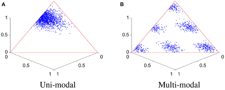
Figure 1. Uni-modal and multi-modal IETs. (A) IETs of a two-event binomial process, with a uni-modal distribution. (B) IETs of another two-event binomial process, with a multi-modal distribution.

However, practical data may have more complicated structures than a uni-modal distribution; that is, a single Dirichlet distribution may not be able to fully characterize the details of the conditional distribution of IETs. Using another binomial point process, its 2000 two-event IET vectors are shown in Figure 1B, where a clear multi-modal distribution is observed. In this article, we further propose to extend the notion of rank-based Dirichlet model to a more general framework—a Dirichlet mixture model, where we model the IETs of a point process (conditioned on the number of events) using a mixture of Dirichlet distributions.

For uni-modal Dirichlet distribution, the parameters in the model can be easily estimated using a classical maximum likelihood approach. However, the estimation is more challenging for a mixture model. In principle, we need to do two estimations: one is on the number of mixture components, and the other is on the parameter values given the component number. We propose to use a Dirichlet process and Expectation-Maximization (EM) algorithm to handle these two estimations, respectively. Dirichlet Process Mixture (DPM) model is a nonparametric mixture model which allows infinitely many components. The method can conduct clustering on observations without model selection. The Dirichlet Process was first presented as a class of prior distributions for nonparametric problems [22], and then extended with the formal definition for Dirichlet Process Mixture [23]. In particular, Markov chain Monte Carlo (MCMC) methods are often used for the purposes of inference and sampling in the DPM model.

For the Dirichlet model, conjugate prior is often not available [24, 25]. In this case, approximations based on Monte Carlo methods can be computationally expensive. In order to take advantage of the conjugate priors and simplify the calculation, instead of modeling IETs directly using a Dirichlet mixture, we also propose an indirect model by adopting the isometric logratio transformation in compositional data analysis [26, 27]. By this bijective transformation, the IETs are transformed to an unconstrained Euclidean space. Then, a classical multivariate Gaussian Mixture model (GMM) can be adopted to model the transformed data. For GMM, the closed-form estimations in the Dirichlet process posterior and EM algorithm are thoroughly studied in Murphy [28] and Bilmes [29] and no approximation is needed.

The rest of this manuscript is organized as follows: In Section 2, we will provide details of the Dirichlet model, Dirichlet mixture model on the IETs and Gaussian mixture model on the transformed IETs. The estimation procedures, including Dirichlet process and EM algorithm will also be given. In Section 3, two simulation experiments will be used to illustrate the center-outward ranking of the proposed models. We will also apply the new methods to conduct a classification task in a real experimental data set. Finally, we will summarize our work in Section 4.

2. Methods

2.1. Likelihood in a Temporal Point Process

Mathematical modeling on the temporal point process has been a central problem in stochastic process. We will at first review the classical theory on point process and then provide a new framework for the likelihood representation.

2.1.1. Review of the Classical Theory

Classical methods have focused on regular point processes, where the event times can be ordered increasingly without overlapping. Only finite number of events are allowed in any finite time interval, and the commonly used conditional intensity function can be well defined. In practical use, point process observations are often in a finite domain and we limit our study in an interval [0, T], where T > 0 denotes the time length.

Assume a temporal point process is given as ${H}=\left\{s_i\right\}$ with $s_i\in {ℝ}^{+}$ and i = 1, 2, ⋯ . Denote the conditional density function $f(s_{n+1}|{{H}}_{s_n})$ of the event time s_n+1 given the history of previous events ${{H}}_{s_n}=(s_1,\cdots ,s_n)$. Using the chain rule of the conditional distribution, the joint density can be represented as follows:

$\begin{array}{l}f(s_1,s_2,\cdots )={\displaystyle \prod _n}f(s_n|s_{n-1},\cdots ,s_1)={\displaystyle \prod _n}f(s_n|{{H}}_{s_{n-1}}).\end{array}$

For any u > s_n, the conditional intensity function is defined in the following form:

$\begin{array}{l}{\lambda }^{*}(u)=\frac{f(u|{{H}}_{s_n})}{1-F(u|{{H}}_{s_n})},\end{array}$

where $F(u|{{H}}_{s_n})={\int }_{s_n}^{u}f(t|{{H}}_{s_n})dt$ is the conditional cumulative distribution function. The conditional intensity function λ^*(u) models the mean number of events in a region conditional on the past, and it can determine the probability structure of a regular point process uniquely [1]. Using λ^*(u), the likelihood of a point process realization (s₁, ⋯ , s_n) on (0, T) is given by

$\begin{array}{l}L=({\displaystyle \prod _{i=1}^n}{\lambda }^{*}(s_i))exp(-{\Lambda }^{*}(T)),\end{array}$

where ${\Lambda }^{*}(u)={\int }_0^u{\lambda }^{*}(t)dt$ is the integrated conditional intensity function.

This time-based description characterizes the probability structure at any time. However, it does not describe the center-outward rank, or relative “importance,” of each realization. For example, for a homogeneous Poisson process (HPP) with constant intensity λ^*(s) = λ, the likelihood is:

$\begin{array}{l}{L}_{HPP}=({\displaystyle \prod _{i=1}^n}\lambda )exp(-{\displaystyle {\int }_0^T}\lambda dt)={\lambda }^{n}exp(\lambda T).\end{array}$

Given the time interval [0, T] and intensity rate λ, the likelihood only depends on n. That is, realizations with the same number of events will have equal likelihood, regardless of their event times. Such likelihood cannot properly define a center-outward rank to indicate the centrality (or outlyingness) of each realization. In the article, we aim to propose a data-driven model on point processes which leads to a proper center-outward rank.

2.1.2. Rank-Based Likelihood Representation

To characterize the overall pattern of a temporal point process s = (s₁, ⋯ , s_n), we need to measure the likelihood of two types of randomnesses: (1) the number of events in the process and (2) the distribution of these events. That is, the likelihood of the process s can also be calculated via the following equation.

$\begin{array}{ll}p(s=(s_1,\cdots ,s_n))=p(|s|=n)·p(s=(s_1,\cdots ,s_n)||s|=n),& (1)\end{array}$

where |s| denotes the cardinality of the sequence s.

Note that |s| is a random variable. For a regular point process on [0, T], p(|s| < ∞) = 1. As |s| is only a one-dimensional counting variable, there are a lot of possible ways to model it such as a parametric Poisson model or a nonparametric model. The key challenge is at the conditional distribution p(s||s|). In the special case of a Poisson process with (history-independent) intensity function λ(t), it is known that $|s|~Poisson\left({\int }_0^T\lambda (t)dt\right),$ and

$s_1,\cdots ,s_n||s|=n\stackrel{\text{i.i.d.}}{~}\frac{\lambda (t)}{{\int }_0^T\lambda (t)dt}.$

A point process, however, in general is history-dependent, and there will be no such explicit formula for the conditional distribution. Parametric models such as Gaussian distribution [9] and Dirichlet distribution [21] can be considered. Our main goal of this article is to provide a rank-based parsimonious model on this conditional distribution which can properly characterize practical observations. This will be clearly given in the following subsections.

2.2. Rank-Based Conditional Model

2.2.1. Dirichlet Model

In this section, we will provide models for the conditional distribution p(s = (s₁, ⋯ , s_d)| |s| = d) in Equation (1). Given the number of events, a parsimonious Dirichlet distribution is proposed to describe the conditional distribution of inter-event times. Note that this model may not describe the true likelihood of the realization, but provides a reasonable data-driven description of the importance or center-outward rank of the given realization. Therefore, the probability representation is actually a “pseudo-likelihood,” and is denoted as $\tilde{p}$.

It is commonly known that a point process can be equivalently represented by their inter-event times (IETs). That is, for a point process with d events 0 < s₁ < s₂ < ⋯ < s_d < T, its IETs are given as u₁ = s₁, u₂ = s₂−s₁, ⋯ , u_d = s_d−s_d−1, u_d+1 = T−s_d. The IET sequence u = (u₁, u₂, ⋯ , u_d+1) forms a d-dimensional simplex (scaled standard simplex) as:

$\begin{array}{l}{{S}}^d=\{(u_1,u_2,\cdots ,u_{d+1})\in {ℝ}^{d+1}:u_1+u_2+\cdots +u_{d+1}\\ =T,u_i\ge 0,i=1,2,\cdots ,d+1\},\end{array}$

which has the same support as a Dirichlet distribution. Therefore, it is natural to adopt a Dirichlet distribution to model the conditional distribution of the IETs as follows.

2.2.1.1. Dirichlet Model

For a point process s = (s₁, ⋯ , s_d) in time interval (0, T), let s₀ = 0 and s_d+1 = T. Then its IET vector $u=(u_1=s_1-s_0,u_2=s_2-s_1,\cdots ,u_{d+1}=s_{d+1}-s_d)\in {ℝ}^{d+1}$ lies on a d-dimensional simplex. We model the conditional distribution of this process using a d+1 dimensional Dirichlet distribution with parameters $\alpha =({\alpha }_1,\cdots ,{\alpha }_{d+1})\in {ℝ}_{+}^{d+1}$ on its IET vector. That is:

$\begin{array}{ll}\tilde{p}(s=(s_1,\cdots ,s_d)||s|=d)=\frac{\Gamma ({\displaystyle {\sum }_{i=1}^{d+1}}{\alpha }_i)}{{\displaystyle {\prod }_{i=1}^{d+1}}\Gamma ({\alpha }_i)}{\displaystyle \prod _{i=1}^{d+1}}{(\frac{u_i}{T})}^{{\alpha }_i-1},& (2)\end{array}$

where Γ(·) is a Gamma function, and α_i > 1 for i = 1, ⋯ , d+1 to guarantee the unique mode in the Dirichlet model.

Based on the IET representation, the Dirichlet model in Equation (2) can naturally take into account the orderedness and boundedness of all events in a point process. In addition, the center of the process can be characterized by the mode of the Dirichlet distribution. In a Dirichlet model, the likelihood reaches the maximum when $u_i=\frac{{\alpha }_i-1}{{\sum }_{j=1}^{d+1}{\alpha }_j-(d+1)}$, i = 1, ⋯ , d+1. Also, it is easy to verify that the likelihood value decreases from the center monotonically. That is, a center-outward rank can be naturally given by the likelihood value.

2.2.2. Model Identification

Given point process observations, we will need to estimate the parameter α of the Dirichlet model in Equation (2). We propose to conduct the conventional Maximum Likelihood Estimate (MLE) procedure. Assume we have observed N independent realizations with d events, that is S = (S₁, S₂, ⋯ , S_N), where S_n = (s_{n, 1}, s_{n, 2}, ⋯ , s_{n, d}). Then the log-likelihood function L(α) is given as follows:

$\begin{array}{l}L(\alpha )=log\tilde{p}(S|\alpha )=log{\displaystyle \prod _{n=1}^N}p(S_n|\alpha )\\ =log{\displaystyle \prod _{n=1}^N}\frac{\Gamma ({\displaystyle {\sum }_{i=1}^{d+1}}{\alpha }_i)}{{\displaystyle {\prod }_{i=1}^{d+1}}\Gamma ({\alpha }_i)}{\displaystyle \prod _{i=1}^{d+1}}{(\frac{s_{n,i}-s_{n,i-1}}{T})}^{{\alpha }_i-1}\\ =N(log\Gamma ({\displaystyle \sum _{i=1}^{d+1}}{\alpha }_i)-{\displaystyle \sum _{i=1}^{d+1}}log\Gamma ({\alpha }_i))\\ +{\displaystyle \sum _{i=1}^{d+1}}({\alpha }_i-1){\displaystyle \sum _{n=1}^N}log(\frac{s_{n,i}-s_{n,i-1}}{T}).\end{array}$

We propose to use the Newton-Raphson (N-R) method to find the maximum of L(α) [30]. In order to use the method, we need to derive the gradient ∇L and Hessian matrix H with respect to the parameter α. The gradient $\nabla L=(\frac{\partial L}{\partial {\alpha }_1},\cdots ,\frac{\partial L}{\partial {\alpha }_{d+1}})$ is obtained by calculating the first-order derivatives:

$\begin{array}{l}\frac{\partial L}{\partial {\alpha }_i}=N(\psi ({\displaystyle \sum _{i=1}^{d+1}}{\alpha }_i)-\psi ({\alpha }_i))+{\displaystyle \sum _{n=1}^N}log(\frac{s_{n,i}-s_{n,i-1}}{T}),\\ i=1,\cdots ,d+1,\end{array}$

where $\psi (x)=\frac{{\Gamma }^{\prime }(x)}{\Gamma (x)}$ is known as the digamma function. To get the Hessian matrix $H={(\frac{{\partial }^{2}L}{\partial {\alpha }_j\partial {\alpha }_i})}_{j,i=1}^{d+1}\in {ℝ}^{(d+1)\times (d+1)}$, we need to calculate the second-order derivatives:

$\frac{{\partial }^{2}L}{\partial {\alpha }_i^2}=N({\psi }^{\prime }({\displaystyle \sum _{i=1}^{d+1}}{\alpha }_i)-{\psi }^{\prime }({\alpha }_i)),i=1,\cdots ,d+1,$

$\frac{{\partial }^{2}L}{\partial {\alpha }_j\partial {\alpha }_i}=N{\psi }^{\prime }({\displaystyle \sum _{i=1}^{d+1}}{\alpha }_i),j,i=1,\cdots ,d+1,j\ne i.$

Note that for a large value of d, the computation of H⁻¹ can be very costly. To make the procedure more efficient, we can rewrite the hessian matrix as H = Q+c11^T, where Q = diag(q₁, ⋯ , q_d+1) with $q_i=-N{\psi }^{\prime }({\alpha }_i)\underset{̣}{,}i=1,\cdots ,d+1$, $c=N{\psi }^{\prime }({\sum }_{i=1}^{d+1}{\alpha }_i)$, and 1 ∈ ℝ^d+1 is a column vector with every entry being 1. It is easy to see that $H^{-1}=Q^{-1}-\frac{Q^{-1}11^T{Q}^{-1}}{1/c+1^T{Q}^{-1}1}$. Therefore, the parameter α can be updated using the following iteration:

${\alpha }^{new}={\alpha }^{old}-(Q^{-1}-\frac{Q^{-1}11^T{Q}^{-1}}{1/c+1^T{Q}^{-1}1})\nabla L.$

The MLE estimate above is for a given number of events d. For a point process, we need to estimate the Dirichlet parameters in each dimension. In practice, we will set an upper bound D and only make estimations for the cases with up to D events.

2.3. Dirichlet Mixture Models

We have proposed to use a Dirichlet model to represent the likelihood of the IETs of a given point process realization. However, the underlying distribution of the IETs of a point process may be more complicated than a unimodal Dirichlet distribution. In this section, we will propose to adopt a mixture model to address this issue.

2.3.1. Mixture of Dirichlet Distribution

We will at first use an example to illustrate the insufficiency of Dirichlet model for complicated IET patterns. In Figure 2A, the scatter plot is the point cloud from a binomial point process with 2 events (see simulation detail in Section 3). A single Dirichlet model (shown with multiple contour lines) cannot properly describe the multi-modal pattern. In Figure 2B, we adopt a mixture of Dirichlet distributions, which apparently provides a more appropriate characterization on the observed IETs.

FIGURE 2

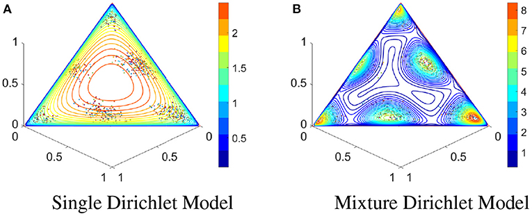
Figure 2. IETs of a binomial point process and contours of Dirichlet models. (A) IETs of simulated binomial point process with 2 events and contours of a fitted single Dirichlet model. (B) Same as (A) except using a Dirichlet mixture model with 6 components.

The Dirichlet mixture model on the conditional distribution of IETs is formally given as follows:

2.3.1.1. Dirichlet Mixture Model

For a point process s given |s| = d in time interval (0, T), let s₀ = 0, s_d+1 = T, and the IETs u = (u₁, u₂, ⋯ , u_d+1) = (s₁−s₀, s₂−s₁, ⋯ , s_d+1−s_d). The conditional distribution of IETs is modeled using a Dirichlet mixture model:

$\begin{array}{l}\tilde{p}(s=(s_1,\cdots ,s_d)||s|=d)={\displaystyle \sum _{k=1}^K}{w}_k\frac{{\displaystyle {\prod }_{i=1}^{d+1}}\Gamma ({\alpha }_{i,k})}{\Gamma ({\displaystyle {\sum }_{i=1}^{d+1}}{\alpha }_{i,k})}{\displaystyle \prod _{i=1}^{d+1}}{(\frac{u_i}{T})}^{{\alpha }_{i,k}-1}\end{array}$

where K denotes the number of the mixture components, w_k is the weight parameter of k^th component, α_{·, k} = (α_{1, k}, ⋯ , α_{d+1, k}) are the parameters of the k^th Dirichlet distribution, k = 1, ⋯ , K.

In practice, we need to estimate parameters in a Dirichlet mixture model for given IETs. To do so, we need to estimate (1) the number of components K and (2) parameters {α_{i, k}} and {w_k} in each component. Estimation of K is a classical model selection problem. We propose to adopt a nonparametric Dirichlet process to find an optimal component number. Once this number is known, we will use an Expectation-Maximization (EM) algorithm to estimate parameters {α_{i, k}} and {w_k}. These two procedures are clearly given in the following subsections.

2.3.2. Model Selection via Dirichlet Process

Dirichlet Process [22] defines a prior distribution for the mixture. In this subsection, we propose to use a Monte-Carlo method to estimate the optimal number of components in the mixture.

2.3.2.1. Prior

Assume the mixture of Dirichlet distributions in Section 2.3.1 has a prior of Dirichlet Process with exponential base distribution G₀ = exp(λ) and a scalar precision parameter γ > 0 for the components concentration. N observations X = {X₁, ⋯ , X_N} are given in the Dirichlet mixture model, where each observation comes from one of the mixture components. Using the Dirichlet process, we can write the prior information of the mixture model as:

$\begin{array}{l}G~DP(\gamma ,G_0=exp(\lambda ))\\ ({\theta }_i|G)~G\\ X_i~Dir({\theta }_i),& (3)\end{array}$

where λ is a hyperparameter of the base distribution G₀, X_i = (x_i1, ⋯ , x_id) is the i^th observation, θ_i = (α_{1, (i)}, ⋯ , α_{d, (i)}) is the parameters of the component that the i^th observation X_i belongs to. Note that if θ_i = θ_j, then the i^th and j^th components are from the same component.

To sample from the posterior distribution easily, we need to introduce the equivalent view of the Dirichlet Process, known as “Chinese Restaurant Process” [31]. Given the Dirichlet process prior we described in Equations (3), the indicator variable follows the Chinese Restaurant Process. That is

$\begin{array}{ll}P(z_i=j|Z^{-i},\gamma )=\frac{n_j^{-i}}{n-1+\gamma }& (4)\end{array}$

$\begin{array}{ll}P(z_i=new|Z^{-i},\gamma )=\frac{\gamma }{n-1+\gamma },& (5)\end{array}$

where z_i is the indicator variable corresponding to the i^th observation, $Z^{-i}=(z_1,\cdots ,z_{i-1},z_{i+1},\cdots ,z_N)$, and $n_j^{-i}$ is the number of observations in (X₁, ⋯ , X_i−1, X_i+1, ⋯ , X_N) belonging to j^th component.

2.3.2.2. Posterior of Indicator

Assume we fix the currently existing component parameters Θ = (θ₁, …, θ_k). Given γ and observations X, the posterior probability of indicators can be written as:

For the existing components:

$\begin{array}{l}P(z_i=j|Z^{-i},X,\Theta )=P(z_i=j|Z^{-i})\\ P(X_i|z_i=j,{\theta }_j)\frac{P(Z^{-i},X^{-i},\Theta )}{P(Z^{-i},X,\Theta )}.& (6)\end{array}$

For the new component:

$\begin{array}{l}P(z_i=new|Z^{-i},X,\Theta )=P(z_i=new|Z^{-i})\\ P(X_i|z_i=new)\frac{P(Z^{-i},X^{-i},\Theta )}{P(Z^{-i},X,\Theta )}.& (7)\end{array}$

Integrating over Θ, we get

$\begin{array}{ll}P(z_i=j|Z^{-i},X)=b·\frac{n_j^{-i}}{n-1+\gamma }·{\displaystyle {\int }_{{\theta }_j}Dir(X_i|{\theta }_j)d{H}_{-i}({\theta }_j)}& (8)\end{array}$

$\begin{array}{ll}P(z_i=new|Z^{-i},X)=b·\frac{\gamma }{n-1+\gamma }·{\displaystyle {\int }_{\theta }}Dir(X_i|\theta )d{G}_0(\theta ),& (9)\end{array}$

where H_−i(θ_j) is the posterior distribution of θ based on the prior G₀ and all observations $X_l\in X^{-i}$, z_l = j, and $b=\frac{P(Z^{-i},X^{-i},\Theta )}{P(Z^{-i},X,\Theta )}$.

2.3.2.3. Non-conjugate Estimation

The integrals in Equations (8) and (9) can be integrated analytically in a conjugate context. Dirichlet and Exponential distributions, however, are not conjugate, and we need to find another method to estimate the posterior distribution of indicators Z = (z₁, ⋯ , z_n) [24]. In this article, we propose to substitute Θ into Equations (6) and (7) to estimate the posterior distribution of Z.

Then for Equation (6)

$\begin{array}{l}P(z_i=j|Z^{-i},X,\Theta )=b·P(z_i=j|Z^{-i})P(X_i|z_i=j,{\theta }_j)\\ =b·\frac{n_j^{-i}}{n-1+\gamma }·Dir(X_i|{\theta }_j).& (10)\end{array}$

When θ_j is available, it is straight forward to obtain the result in Equation (10). For Equation (7)

$\begin{array}{l}P(z_i=new|Z^{-i},X,\Theta )=b·P(z_i=new|Z^{-i})P(X_i|z_i=new)\\ =b·\frac{\gamma }{n-1+\gamma }·{\displaystyle {\int }_{\theta }}Dir(X_i|\theta )d{G}_0(\theta )& (11)\end{array}$

In Equation (11), the integral term is on one sample X_i. Therefore, a Monte-Carlo method can be adopted. We will generate M samples of θ from G₀, denoted as ${\left\{{\theta }_i\right\}}_{i=1}^M$, and then estimate the integral term as.

$\begin{array}{ll}{\displaystyle {\int }_{\theta }}Dir(X_i|\theta )d{G}_0(\theta )=\frac{1}{M}{\displaystyle \sum _{i=1}^M}Dir(X_i|{\theta }_i).& (12)\end{array}$

2.3.2.4. Maximum a Posteriori (MAP) for Estimating Θ

Next, we will use the MAP to estimate the new θ_j after each iteration. The likelihood with the prior knowledge is

$\begin{array}{l}L({\theta }_j)=p(X|{\theta }_j)p({\theta }_j)={\displaystyle \prod _i}Dir(X_i|{\theta }_j)exp({\theta }_j)\\ ={\displaystyle \prod _{i=1}^{n_j}}(\frac{\Gamma ({\displaystyle {\sum }_{k=1}^d}{\alpha }_{j,k})}{{\displaystyle {\prod }_{k=1}^d}\Gamma ({\alpha }_{j,k})}{\displaystyle \prod _{k=1}^d}{x}_{ik}^{{\alpha }_{j,k}-1}){\displaystyle \prod _{k=1}^d}{\lambda }_k{e}^{-{\lambda }_k{\alpha }_{j,k}}.\end{array}$

Hence, the log-likelihood is

$\begin{array}{l}l({\theta }_j)=n_j(\log \Gamma ({\displaystyle \sum _{k=1}^d{\alpha }_{j,k}})-{\displaystyle \sum _{k=1}^d\log }\Gamma ({\alpha }_{j,k})\\ +{\displaystyle \sum _{k=1}^d(}{\alpha }_{j,k}-1)\log {\widehat{X}}_k)-{\displaystyle \sum _{k=1}^d{\lambda }_k}{\alpha }_{j,k}+constant,& (13)\end{array}$

where {X₁, X₂, …, X_nj} is a set of observed multinomial data in component j, and $log{\widehat{X}}_k=\frac{1}{n_j}{\sum }_{i}log{x}_{ik}$. Similar to Section 2.2.2, we can use the Newton-Raphson's method to find the maximum of l(θ). The details are omitted here.

So far we have sampled Dirichlet Mixture Distributions from the posterior DP iteratively. For each sample, we have a number of components. Therefore, we obtain an empirical distribution of number of components and an “optimal” number of components for the given data can be taken as the mean, median, or mode of the distribution thereafter. In practice, such distribution often has a narrow range of optimal values. The MCMC algorithm is given in Algorithm 1 as follows, where NumOfComponents denotes the number of components for the given data.

ALGORITHM 1

Algorithm 1. Dirichlet Process to Estimate the Number of Components.

2.3.3. Model Identification via EM Algorithm

Once an optimal number of events is estimated using the Dirichlet process, we can estimate parameters in the Dirichlet mixture model. This estimation can be effectively done with an EM algorithm.

Let S = {s₁, s₂, ⋯ , s_N} denote N observed realizations with d events. Their equivalent representations using IETs are denoted by U = {u₁, ⋯ , u_N} in simplex ${{S}}^d\subset {ℝ}^{d+1}$. We will model these IETs using a Dirichlet mixture model with K components. The likelihood of all observations is given as

$\begin{array}{ll}f(U|\theta )={\displaystyle \prod _{i=1}^N}{\displaystyle \sum _{k=1}^K}{w}_k{f}_k(u_i|{\alpha }_{·,k}),& (14)\end{array}$

where $\theta =({\left\{w_k,{\alpha }_{·,k}\right\}}_{k=1}^K)$ denote all parameters with w_k being the weight coefficient and α_{·, k} = (α_{0, k}, ⋯ , α_{d, k}) in the density of Dirichlet distribution f_k, k = 1, ⋯ , K. We use Z = {Z₁, Z₂, ⋯ , Z_N} to denote the missing labels of all observations, where Z_i = (z_{i, 1}, ⋯ , z_{i, K}) with

$\begin{array}{l}{z}_{i,k}=\{\begin{array}{cc}1& \text{if }{u}_i\text{ belongs to the }k\text{th component}\\ 0& \text{otherwise}.\\ \end{array}\end{array}$

2.3.3.1. E-Step

Our goal is to maximize f(U|θ). Based on conditional representation f(U, Z|θ) = f(U|θ)f(Z|U, θ), we get

$logf(U|\theta )=logf(U,Z|\theta )-logf(Z|U,\theta ).$

Taking expectation on both side with respect to the density function f(Z|U, θ^(m)) for estimate θ^(m) after m-th iteration, we have

$E\left[logf(U|\theta )\right]=Q(\theta |{\theta }^{(m)},U)-H(\theta |{\theta }^{(m)},U),$

where Q(θ|θ^(m), U) = E[logf(U, Z|θ)|θ^(m), U] and H(θ|θ^(m), U) = E[logf(Z|U, θ)|θ^(m), U].

According to (14), the Q function can be written as.

$\begin{array}{l}Q(\theta |{\theta }^{(m)},U)=E[\log f(U,Z|\theta )|{\theta }^{(m)},U]\\ ={\displaystyle \sum _{i=1}^N(}{\displaystyle \sum _{k=1}^K[log{w}_k}log\Gamma ({\displaystyle \sum _{d=1}^D{\alpha }_{d,k})}\\ -{\displaystyle \sum _{d=1}^{D}l}og\Gamma ({\alpha }_{d,k})\\ +{\displaystyle \sum _{d=1}^D({\alpha }_{d,k}-1)}log{u}_{i,d}]P(k|u_i,{\theta }^{(m)})).& (15)\end{array}$

2.3.3.2. M-Step

We will update {α_{d, k}} to maximize Q function by solving

$\begin{array}{ll}\frac{\partial Q}{\partial {\alpha }_{d,k}}={\displaystyle \sum _{i=1}^N}(\frac{{\Gamma }^{\prime }({\displaystyle {\sum }_d}{\alpha }_{d,k})}{\Gamma ({\displaystyle {\sum }_d}{\alpha }_{d,k})}-\frac{{\Gamma }^{\prime }({\alpha }_{d,k})}{\Gamma ({\alpha }_{d,k})}+log{u}_{i,d})P(k|u_i,{\theta }^{(m)})=0& (16)\end{array}$

with the Newton-Raphson method. Update {w_k} by solving

$\begin{array}{ll}\frac{\partial g}{\partial w_k}={\displaystyle \sum _{i=1}^N}\frac{P(k|u_i,{\theta }^{(m)})}{w_k}+\lambda =0,& (17)\end{array}$

where

$g=Q+\lambda ({\displaystyle \sum _{k=1}^K}{w}_k-1)$

and λ is the Lagrange multiplier.

In summary, the EM-algorithm is given in Algorithm 2 as follows.

ALGORITHM 2

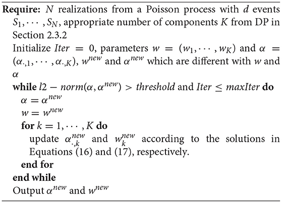
Algorithm 2. Parameter Estimation using the EM Algorithm.

2.3.4. Multiple Mixture Models

When the number of events, d, is given in the point process, we have proposed a combination of Dirichlet process and EM algorithm to estimate the parameters in the model. However, point process data often have observations with various numbers of events, and we need to estimate a model for each case. In practice, we can set an upper bound D, and only estimate models with number of events up to D. To make the estimation procedure feasible, we will only use Dirichlet process to estimate the number of mixture components for d = D, and then use the same component number for d = 1, ⋯ , D − 1. To identify these mixture models, the EM algorithm will be used for each value of d = 1, ⋯ , D. We use w_k:d to denote the weight parameter and α_{·, k:d} to denote the Dirichlet parameters for k^th component in d dimensional cases. The algorithm is shown below.

2.4. Alternative Mixture Model

In Subsection 2.3, we have proposed a Dirichlet Mixture Model to describe the conditional distribution of IETs of a point process. Dirichlet distribution has the same support as IETs so that it is suitable for the IET modeling. However, the Dirichlet process and EM algorithm for the mixture Dirichlet distributions have no closed-form updates. We choose to rely on Monte Carlo or gradient methods to approximate the solutions, which are computationally expensive. In this subsection, we introduce an alternative approach based on compositional data analysis. Firstly, we apply the bijective isometric logratio transformation (ilr) [26] to map the IETs from D-dimensional simplex ${{S}}^D$ to ℝ^D−1. Then a Gaussian Mixture model can be utilized to characterize the distribution of transformed IETs in the Euclidean space and we can take advantages of the conjugate prior with closed-form solutions.

2.4.1. Isometric Logratio Transformation and Gaussian Mixture Model

Compositional data is fundamentally different from unconstrained multivariate data that it has a constant sum constraint [27]. The bijective logratio transformation methods such as centered logratio transformation (clr) and isometric logratio transformation (ilr) [32] have been successfully used to deal with such type of data. They transform the original data to an unconstrained space, making it possible to use various conventional multivariate models on the transformed data. The isometric logratio transformation is a preferred version of such transformation with the apparent advantages such as distance and angle preserving and full rank covariance. Given $X=(x_1,x_2,\cdots ,x_D)\in {{S}}^D$, we can denote the centered logratio transformation as:

$\begin{array}{l}clr(X)=(ln\frac{x_1}{g(X)},ln\frac{x_2}{g(X)},\cdots ,ln\frac{x_D}{g(X)}),\end{array}$

where $g(X)={({\prod }_{i=1}^D{x}_i)}^{1/D}$ is the component-wise geometric mean. Together with an appropriate clr-matrix of the orthonormal basis, Ψ ∈ ℝ^{D × (D−1)}, the isometric logratio transformation can be expressed as:

$\begin{array}{ll}ilr(X)=clr(X)·{\text{Ψ}}^{\prime }.& (18)\end{array}$

Gram-Schmidt techniques [26] can be utilized to obtain an appropriate orthonormal basis of the simplex easily. The entries of Ψ can be expressed as:

$\begin{array}{ll}{\text{Ψ}}_{i,j}=\{\begin{array}{cc}\hfill \sqrt{\frac{1}{(D-i)(D-i+1)}},& j\le D-i,\hfill \\ \hfill -\sqrt{\frac{D-i}{D-i+1}},& j=D-i+1,\hfill \\ \hfill 0,& \text{otherwise}.\hfill \end{array}& (19)\end{array}$

Assuming we have N observations and their corresponding IETs U = {u₁, ⋯ , u_N} in simplex ${{S}}^d$, the ilr transformation can help remove the constant-sum constraint of U by mapping it to an unconstrained Euclidean space ℝ^d−1, i.e., $ilr(U)={\left\{ilr(u_i)\right\}}_{i=1}^N\subset {ℝ}^{d-1}$. Because of its isometric property, the clustering components will be preserved (See one example in Figure 3). This makes the commonly used Gaussian Mixture model appropriate for ilr(U).

FIGURE 3

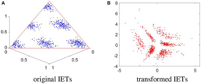
Figure 3. 2-event IETs on simplex and transformed IETs on Euclidean space. (A) Scatter plot for the original IETs on the 3-D simplex. (B) Transformed IETs after ilr transformation in the 2-D Euclidean space.

After removing the constant sum restriction, the transformed IET vector ilr(U) is in an unconstrained Euclidean space so that the classical multivariate Gaussian Mixture model (GMM) can be used directly. For a given process, we firstly conduct the ilr transformation, and then fit a GMM on the transformed data. This modeling procedure is given as follows:

2.4.1.1. Gaussian Mixture Model

For a point process s given |s| = d in time interval [0, T), let s₀ = 0, s_d+1 = T, and the IET vector u = (u₁, u₂, ⋯ , u_d+1) = (s₁−s₀, s₂−s₁, ⋯ , s_d+1−s_d). Using the ilr transformation, we have u^* = ilr(u) ∈ ℝ^d−1, the conditional distribution of point process is modeled using a Gaussian mixture model on u^*:

$\begin{array}{l}\tilde{p}(s=(s_1,\cdots ,s_n)||s|=n)\\ ={\displaystyle \sum _{k=1}^K{w}_k}\frac{1}{{(2\pi )}^{(d-1)/2}|{\sum }_k{|}^{(1/2)}}\\ \exp (-\frac{1}{2}{(u^{*}-{\mu }_k)}^T{\sum }_k^{-1}(u^{*}-{\mu }_k))\end{array}$

where K denotes the number of the mixture components, w_k is the weight parameter of k^th component, and ${\mu }_k\in {ℝ}^{d-1}$ and ${\Sigma }_k\in {ℝ}^{(d-1)\times (d-1)}$ are the mean and covariance of the k^th Gaussian distribution, respectively, k = 1, ⋯ , K.

For a given number of events d, we still use the Dirichlet Process to conduct the model selection and EM-algorithm to estimate the mixture model parameters. For observations with various number of events, we follow the same procedure in Algorithm 3 to identify Gaussian mixture models for each dimension. The details are given in the following subsections.

ALGORITHM 3

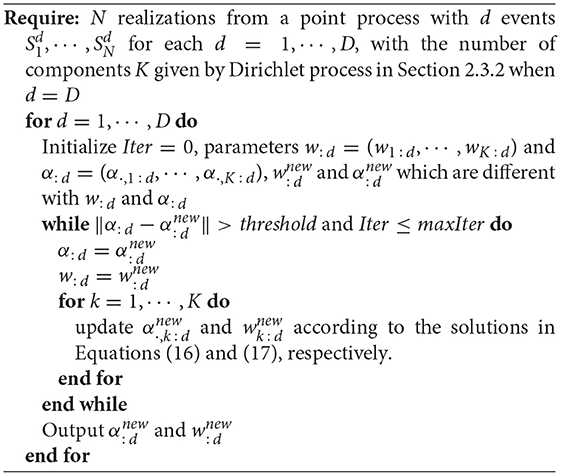
Algorithm 3. Estimate Parameters for Multiple Dirichlet Mixture Models.

2.4.2. Dirichlet Process on Gaussian Mixture Model

Dirichlet process Gaussian mixture model (DPGMM) [33] is a classical Dirichlet process mixture model. We can naturally choose the conjugate priors for the mean and precision matrix (inverse of covariance matrix) to get a closed-form posterior. For a Gaussian distribution N(μ_i, R_i) with mean μ_i and precision R_i, we assume the joint distribution of (μ_i, R_i) has a Normal-Wishart distribution, denoted as

$({\mu }_i,R_i)~NW(\kappa ,m,\nu ,U),$

where m and κR_i are the mean and precision of the Normal prior; ν and U are the parameters of the Wishart prior. The DP can be written as:

$\begin{array}{l}G~DP(\gamma ,NW({\kappa }_0,m_0,{\nu }_0,U_0))\\ ({\theta }_i|G)~G\\ X_i~N({\theta }_i),& (20)\end{array}$

where κ₀, m₀, ν₀, U₀ are four hyperparameters of the base distribution G₀, X_i = (x_i1, ⋯ , x_id) is the i^th observation, θ_i = (μ_{·, (i)}, R_(i)) is the mean and precision of the component that the i^th observation X_i belongs to.

With this conjugate prior base distribution, the integral parts in Equations (8) and (9) can be calculated analytically. Meanwhile, the posterior distribution of component parameters Θ will also be a Normal-Wishart distribution and the parameters κ, m, ν, U|X can be expressed in closed-forms [28]. Instead of calculating the MAP estimation of Θ, we can sample from the posterior directly. The algorithm is summarized as follows:

In Algorithm 4, we can take advantage of the closed-form solutions to avoid estimating the integral in Equations (10) and (11) without using Monte Carlo method or Newton-Raphson numerical approximation. It can lead to more accurate and efficient sampling procedure for the posterior distribution.

ALGORITHM 4

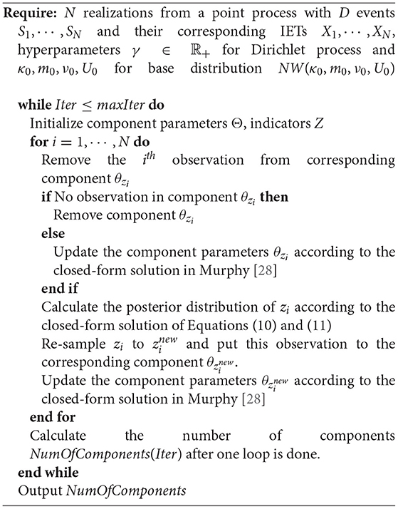
Algorithm 4. Dirichlet Process Gaussian Mixture Model (DPGMM).

2.4.3. EM Algorithm on Gaussian Mixture Model

Gaussian Mixture Model (GMM) is one of the most classical examples for model estimation by the EM algorithm. The closed-form update is well studied in many articles [29]. We will only list the update equations and omit the details.

2.4.3.1. E-Step

For observation $u_i^{*}$, the posterior probability for component k is given by:

$z_{i,k}=P(k|u_i^{*},{\mu }_k,{\Sigma }_k)=\frac{w_{k}N(u_i^{*}|{\mu }_k,{\Sigma }_k)}{{\displaystyle {\sum }_{k=1}^K}{w}_{k}N(u_i^{*}|{\mu }_k,{\Sigma }_k)}$

2.4.3.2. M-Step

The updated parameters $w_k^{new}$, ${\mu }_k^{new}$, and ${\Sigma }_k^{new}$ are given by:

$\begin{array}{l}{w}_k^{new}=\frac{1}{N}{\displaystyle \sum _{i=1}^N}{z}_{i,k}\\ {\mu }_k^{new}=\frac{{\displaystyle {\sum }_{i=1}^N}{z}_{i,k}{u}_i^{*}}{{\displaystyle {\sum }_{i=1}^N}{z}_{i,k}}\\ {\Sigma }_k^{new}=\frac{{\displaystyle {\sum }_{i=1}^N}{z}_{i,k}(u_i^{*}-{\mu }_k^{new}){(u_i^{*}-{\mu }_k^{new})}^T}{{\displaystyle {\sum }_{i=1}^N}{z}_{i,k}}& (21)\end{array}$

We point out that although the closed-form solutions for GMM can make Dirichlet Process and EM algorithm more efficient to calculate, the second-order covariance matrices need to be estimated. This may not be robust when sample size is small. In this study, we will use both DMM on the original IETs and GMM on the transformed IETs, and compare their performance on simulations and real data in the next section.

3. Experimental Studies

In this section, we will at first show a simulation study on a homogeneous Poisson process (HPP) to illustrate the center-outward ranking of our models. We will then examine the likelihood contours and classification performances to show the advantage of the mixture models on simulated inhomogeneous Poisson processes (IPPs). Finally, both Dirichlet Mixture model and Gaussian Mixture model will be evaluated on a real experimental dataset.

3.1. Example 1: Homogeneous Poisson Process (HPP)

We set the upper bound of number of events to be D = 10. For every dimension d ∈ {1, 2, ⋯ , 10}, 1,000 realizations are generated from an HPP. Once we get enough data for all dimensions, Gaussian models and Dirichlet models can be fitted, respectively. In this HPP example, we fit single Dirichlet model and Gaussian model by maximum likelihood estimation (MLE) method.

Figure 4A shows the single Dirichlet model fitted by 1,000 2-event realizations from the HPP. It is clear that the points near the center of the simplex have a higher likelihood. Figure 4B illustrate the corresponding center-outward ranking performance for the top 5 and bottom 5 processes using the single Dirichlet model. It is clear that realizations with evenly distributed events tend to have higher ranks. Similarly, the single Gaussian model likelihood contour and ranking pattern are shown in Figures 4C,D, respectively. Here we fit the single Gaussian models on the transformed IETs in Euclidean space at first, and then transform the IETs and contours back to the simplex space.

FIGURE 4

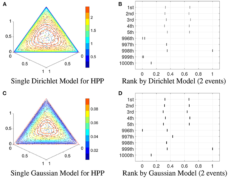
Figure 4. Single models on HPP. (A) Contour of single Dirichlet model for 2-event realizations. (B) Center-outward rank given by the single Dirichlet model for 2-event realizations. (C,D) Same as (A,B) except for the Gaussian model.

To further evaluate the ranking performance, 1,000 realizations with 5 events are tested on the well-trained Dirichlet and Gaussian model and sorted by the likelihood. Figure 5 shows the center-outward ranking of these realizations. We can see the ranking results based on Dirichlet model and Gaussian model are very similar in the five top-ranked and the five bottom-ranked realizations. This indicates both methods produce similar ranks for “central” realizations, as well as similar ranks for extreme outliers.

FIGURE 5

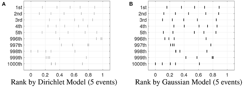
Figure 5. Center-outward Rank given by the models. (A) Center-outward rank given by the single Dirichlet model for 5-event realizations. (B) Same as (A) except for the Gaussian model.

3.2. Example 2: Inhomogeneous Poisson Processes (IPPs)

We generate N = 1, 000 realizations from each of four IPPs on [0, 1] with intensity functions given below:

$\begin{array}{l}{\lambda }_{ipp1}=5·\frac{1}{\sqrt{2\pi }·0.1}·(\exp (-\frac{1}{2}{(\frac{t-0.3}{0.1})}^2)\\ {\lambda }_{ipp2}=5·\frac{1}{\sqrt{2\pi }·0.1}·(\exp (-\frac{1}{2}{(\frac{t-0.7}{0.1})}^2)\\ +\exp (-\frac{1}{2}{(\frac{t-0.66}{0.05})}^2)+\exp (-\frac{1}{2}{(\frac{t-0.9}{0.05})}^2))\\ {\lambda }_{ipp3}=2·\frac{1}{\sqrt{2\pi }·0.05}·(\exp (-\frac{1}{2}{(\frac{t-0.1}{0.05})}^2)\\ +\exp (-\frac{1}{2}{(\frac{t-0.5}{0.05})}^2)\\ +\exp (-\frac{1}{2}{(\frac{t-0.9}{0.05})}^2))\\ {\lambda }_{ipp4}=1.5·\frac{1}{\sqrt{2\pi }·0.05}·(\exp (-\frac{1}{2}{(\frac{t-0.1}{0.05})}^2)\\ +\exp (-\frac{1}{2}{(\frac{t-0.33}{0.05})}^2)\\ +\exp (-\frac{1}{2}{(\frac{t-0.66}{0.05})}^2)+\exp (-\frac{1}{2}{(\frac{t-0.9}{0.05})}^2)),\end{array}$

where the first two intensity functions are uni-modal and the last two are multi-modal. Figure 6 shows all intensity functions.

FIGURE 6

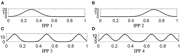
Figure 6. Intensities of four inhomogeneous Poisson processes. (A) The intensity of the first IPP. (B–D) Same as (A) except for the other three processes, respectively.

3.2.1. Uni-Modal Cases

For processes IPP1 and IPP2, we still use single models to describe the IETs' distribution and use MLE method to identify the models. Their IETs of 2-events realizations are shown in Figure 7. It is clear to see that in each process, the IETs are clustering together to one class on the 3-D simplex ${{S}}^3$. Therefore, it is natural to use a Dirichlet distribution to model the likelihood of IETs. Instead of modeling the intensity of each process, our models describe the distribution of the IETs.

FIGURE 7

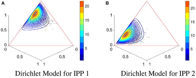
Figure 7. Uni-modal IETs of 2-event realizations for IPP1 and IPP2 and single Dirichlet models. (A) 1,000 2-event realizations of IPP1 and the fitted single Dirichlet model with contours. (B) Same as (A) except for IPP2.

Figure 8 illustrates the ilr-transformation-based approach to model the IETs. Figures 8A,C show the ilr-transformed IETs with the fitted Gaussian contours in these two processes, respectively. Panels (b) and (d) show the corresponding original IETs and the contours transformed back to 3-D simplex from the 2-D Gaussian contours. The shapes of the contours look different from the single Dirichlet models in Figure 7, whereas both methods can properly represent single cluster patterns in the given IETs.

FIGURE 8

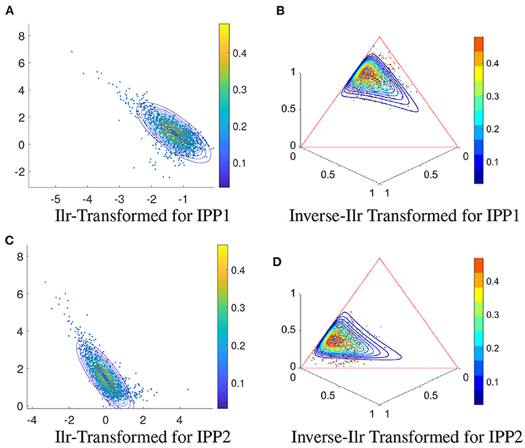
Figure 8. Uni-modal IETs of 2-event realizations for IPP1 and IPP2 and single Gaussian models: (A) Ilr-transformed realizations of IPP1 given in Figure 7A and the fitted Gaussian contours. (B) Original realizations of IPP1 and ilr-inverse-transformed contours from the Gaussian contours in (A). (C,D) Same as (A,B) except for IPP2.

3.2.2. Multi-Modal Cases

For processes IPP3 and IPP4, we model the IETs using mixture models. To fit the models, firstly we do the Dirichlet Process model selection based on Algorithms 1 and 4 to get the optimal number of components. Then, the mixture models are identified by the EM method according to Algorithm 3.

Figures 6C,D are two IPPs with multi-modal intensity functions. In these cases, we use Algorithm 3 to fit Gaussian mixture and Dirichlet mixture models on each dimension. Dirichlet mixture contours with 2-event cases are shown in Figure 9. Similarly to Figures 8B,D, these 2-event realizations with the ilr-inverse-transformed contours are shown in Figure 10.

FIGURE 9

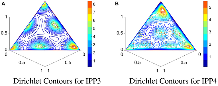
Figure 9. Dirichlet mixture models on IPPs. (A) 1,000 2-event realizations of IPP3 and the density contours by using the Dirichlet mixture model. (B) Same as (A) except for IPP4.

FIGURE 10

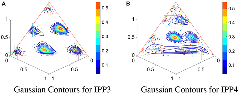
Figure 10. Gaussian mixture models on IPPs: (A) 1,000 2-event realizations from the original 1,000 realizations of IPP3, and the density contours by using the Gaussian mixture model. (B) The same as (A) except for IPP4.

It is easy to see from Figures 9, 10 that these IETs have a clear multi-modal distribution on the simplex, and therefore the single uni-modal distribution cannot describe the distribution appropriately. We adopt the Dirichlet and Gaussian mixture models to characterize the multi-modality. Figure 9 shows that the contours of the Dirichlet mixture model can properly fit the multi-modal pattern. As a comparison, Figure 10 shows the contours of the Gaussian mixture model, which also has the ability to describe the multi-modal pattern, but it is more sensitive to the number of points in each cluster. We can see the contours' shapes fit the data well, whereas the value of likelihoods is very sensitive to the density and location of the points. The clusters at the corner of the triangle tend to have lower likelihood than those at the center. This may be due to the ilr transformation which bijectively maps the cluster points near boundaries of the simplex to sparse points in the unbounded Euclidean space and a Gaussian model on these sparse points can be sensitive to outliers.

In order to demonstrate the advantage of the mixture models, we conduct a classification comparison by using all four models (single Dirichlet, single Gaussian, Dirichlet mixture, and Gaussian mixture). Another 20,000 realizations from IPP3 and IPP4 were generated respectively as the test set. For each realization, we feed it to the four models we proposed. In each case, the label with higher likelihood will be the predicted label of this realization. The classification result of these models is shown in Figure 11. We can see the two mixture models have much higher accuracies for any given number of events (varying from 1 to 10) than the two single models. This result illustrates that the mixture models do have a better representation for data with multi-modal structures.

FIGURE 11

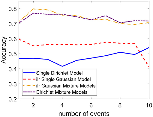
Figure 11. Classification accuracy for each method with respect to the number of events.

3.3. Real Data

In additional to the simulation examples shown above, we will apply these new models on a real experimental recording. This recording was previously used and clearly described in Wu and Srivastava [34]. Briefly, a juvenile male macaque monkey was trained to perform a closed Squared-Path (SP) task by moving a cursor to targets via contralateral arm movements in the horizontal plane. In each trial the subject reached a sequence of five targets consists of the four corners of the square counterclockwise with the first and last one overlapped. If we label the upper left corner as A, lower left as B, lower right as C, and upper right as D, then there will be four different paths, namely, Path 1: ABCDA, Path 2: BCDAB, Path 3: CDABC, and Path 4: DABCD. During the movement, silicon microelectrode arrays were implanted in the arm area of primary motor cortex in the monkey. Signals were filtered, amplified and recorded digitally and single units were manually extracted. There are 60 trials for each path with time length 5–6 s. To fit the models, all these 240 trials were normalized to 5 s. Figure 12 shows 10 trials of spike trains from each path.

FIGURE 12

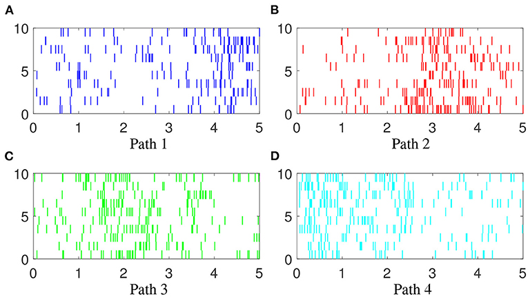
Figure 12. Examples of spike trains. 10 examples of spike trains generated from each path. The four colors (blue, red, green and cyan) indicate spiking activity during hand movement in Paths 1, 2, 3, and 4, (A–D), respectively. Each vertical line represents one event. Each row represents one trial.

For the 60 trials in each path, we randomly select 45 trials as the training data and use the other 15 trials as the test data. The number of events of the 240 trials varies between 12 to 61. It is not robust to train a mixture model for each number of events with such small samples. Therefore, for each trial in the training data, we resample 10 events randomly and use this 10-event realization as one training sample. 10 resampled realizations are randomly generated from each training trial so that we have 45 × 10 = 450 training samples for each path, which are sufficient for the training purpose in this study.

In the training stage, for each path, 450 samples with 10 events described above are used to fit a Dirichlet mixture model and a Gaussian mixture model, respectively. The classification on the test stage is also done for these two models. In the Dirichlet case, we sample 500 10-event realizations for each trial and then fit them to all four Dirichlet mixture models. For each realization, we have 4 likelihoods representing Paths 1, 2, 3, and 4, respectively, and the one with the largest likelihood will be the label of this realization. As a result, 500 labels can be calculated for each trial and the mode will be used as the final label of this trial. The same procedure also applies to the Gaussian case.

Figure 13 are the confusion matrices of Dirichlet and Gaussian mixture models to summarize the classification result. We can see that both methods can identify the trials from Paths 1, 3 and 4 almost perfectly, but perform a little bit worse on identifying trials from Path 2. The overall accuracy of Dirichlet mixture model is 88.33% and of Gaussian mixture model is 86.67%. This result is comparable with the state-of-the-art nearest neighbor method [35].

FIGURE 13

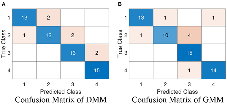
Figure 13. Confusion matrices in 60 testing trials (15 trials for each path). (A) The confusion matrix of the Dirichlet mixture model. (B) The confusion matrix of the Gaussian mixture model.

4. Summary

Instead of estimating the conditional intensity function, we have proposed an alternative approach to model the point process using two factors: (1) the number of events in the process, and (2) the conditional distribution of these events given the number. Our study focuses on the conditional distribution and two approaches are given in this study. One approach adopts Dirichlet distribution to describe the conditional distribution by modeling the equivalent inter-event time representation. To fit more complicated multi-modal distribution of IETs, we extend the notion of rank-based Dirichlet model to rank-based Dirichlet mixture model. The other approach is based on Gaussian model or Gaussian mixture models on the transformed IETs using isometric logratio transformation. This is to avoid the computational inefficiency in the Dirichlet method. In the model fitting stage, we have proposed to use Dirichlet processes to identify the number of components in the mixture models and well-known Expectation-Maximization algorithms for parameter estimations.

This novel, data-driven, rank-based modeling framework can naturally provide a center-outward rank to the realizations, and it is easy to be fitted given enough data. For practical application, realizations from Poisson processes and real experimental recording of spike trains are used to investigate the center-outward ranking and classification performances. In multi-modal cases, it shows that the mixture models offer a more appropriate description and better classification performances than single models. Further applications such as outlier detection will be studied in the future. In addition, we will explore other modeling approaches than the Gaussian mixtures on the transformed IETs.

Data Availability Statement

The original contributions presented in the study are included in the article, further inquiries can be directed to the corresponding author.

Author Contributions

All authors listed have made a substantial, direct, and intellectual contribution to the work and approved it for publication.

Conflict of Interest

The authors declare that the research was conducted in the absence of any commercial or financial relationships that could be construed as a potential conflict of interest.

Publisher's Note

All claims expressed in this article are solely those of the authors and do not necessarily represent those of their affiliated organizations, or those of the publisher, the editors and the reviewers. Any product that may be evaluated in this article, or claim that may be made by its manufacturer, is not guaranteed or endorsed by the publisher.

References

1. Daley DJ, Vere-Jones D. An Introduction to the Theory of Point Processes: Volume I: Elementary Theory and Methods. Probability and Its Applications. New York, NY: Springer (2003).

Google Scholar

2. Brown L, Gans N, Mandelbaum A, Sakov A, Shen H, Zeltyn S, et al. Statistical analysis of a telephone call center: a queueing-science perspective. J Am Stat Assoc. (2005) 100:36–50. doi: 10.1198/016214504000001808

CrossRef Full Text | Google Scholar

3. Rasmussen JG. Lecture notes: temporal point processes and the conditional intensity function. arXiv preprint arXiv:180600221. (2018).

Google Scholar

4. Rubin I. Regular point processes and their detection. IEEE Trans Inf Theory. (1972) 18:547–57. doi: 10.1109/TIT.1972.1054897

CrossRef Full Text | Google Scholar

5. Whitt W. Approximating a point process by a renewal process, I: two basic methods. Oper Res. (1982) 30:125–47. doi: 10.1287/opre.30.1.125

CrossRef Full Text | Google Scholar

6. Hawkes AG. Hawkes processes and their applications to finance: a review. Quant Finance. (2018) 18:193–8. doi: 10.1080/14697688.2017.1403131

CrossRef Full Text | Google Scholar

7. Brown EN, Frank LM, Tang D, Quirk MC, Wilson MA. A statistical paradigm for neural spike train decoding applied to position prediction from ensemble firing patterns of rat hippocampal place cells. J Neurosci. (1998) 18:7411–25. doi: 10.1523/JNEUROSCI.18-18-07411.1998

PubMed Abstract | CrossRef Full Text | Google Scholar

8. Kass RE, Ventura V. A spike-train probability model. Neural Comput. (2001) 13:1713–20. doi: 10.1162/08997660152469314

PubMed Abstract | CrossRef Full Text | Google Scholar

9. Liu S, Wu W. Generalized Mahalanobis depth in point process and its application in neural coding. Ann Appl Stat. (2017) 11:992–1010. doi: 10.1214/17-AOAS1030

CrossRef Full Text | Google Scholar

10. Tukey JW. Mathematics and the picturing of data. In: Proceedings of the International Congress of Mathematicians, Vol. 2. Vancouver, BC (1975). p. 523–31.

Google Scholar

11. Liu RY. On a notion of data depth based on random simplices. Ann Stat. (1990) 18:405–14. doi: 10.1214/aos/1176347507

CrossRef Full Text | Google Scholar

12. Liu RY, Singh K. A quality index based on data depth and multivariate rank tests. J Am Stat Assoc. (1993) 88:252–60. doi: 10.1080/01621459.1993.10594317

CrossRef Full Text | Google Scholar

13. Fraiman R, Liu RY, Meloche J. Multivariate density estimation by probing depth. Lecture Notes Onogr Ser. (1997) 31:415–30. doi: 10.1214/lnms/1215454155

PubMed Abstract | CrossRef Full Text | Google Scholar

14. Zuo Y, Serfling R. General notions of statistical depth function. Ann Stat. (2000) 28:461–82. doi: 10.1214/aos/1016218226

CrossRef Full Text | Google Scholar

15. Cuevas A, Febrero M, Fraiman R. Robust estimation and classification for functional data via projection-based depth notions. Comput Stat. (2007) 22:481–96. doi: 10.1007/s00180-007-0053-0

CrossRef Full Text | Google Scholar

16. López-Pintado S, Romo J. On the concept of depth for functional data. J Am Stat Assoc. (2009) 104:718–34. doi: 10.1198/jasa.2009.0108

CrossRef Full Text | Google Scholar

17. López-Pintado S, Romo J. A half-region depth for functional data. Comput Stat Data Anal. (2011) 55:1679–95. doi: 10.1016/j.csda.2010.10.024

CrossRef Full Text | Google Scholar

18. Claeskens G, Hubert M, Slaets L, Vakili K. Multivariate functional halfspace depth. J Am Stat Assoc. (2014) 109:411–23. doi: 10.1080/01621459.2013.856795

CrossRef Full Text | Google Scholar

19. Helander S, Van Bever G, Rantala S, Ilmonen P. Pareto depth for functional data. Statistics. (2020) 54:182–204. doi: 10.1080/02331888.2019.1700418

CrossRef Full Text | Google Scholar

20. Nieto-Reyes A, Battey H. A topologically valid definition of depth for functional data. Stat Sci. (2016) 31:61–79. doi: 10.1214/15-STS532

CrossRef Full Text | Google Scholar

21. Qi K, Chen Y, Wu W. Dirichlet depths for point process. Electron J Stat. (2021) 15:3574–610. doi: 10.1214/21-EJS1867

PubMed Abstract | CrossRef Full Text | Google Scholar

22. Ferguson TS. A Bayesian analysis of some nonparametric problems. Ann Statist. (1973) 1:209–30. doi: 10.1214/aos/1176342360

CrossRef Full Text | Google Scholar

23. Antoniak CE. Mixtures of Dirichlet processes with applications to Bayesian nonparametric problems. Ann Statist. (1974) 2:1152–74. doi: 10.1214/aos/1176342871

CrossRef Full Text | Google Scholar

24. Neal RM. Markov chain sampling methods for Dirichlet process mixture models. J Comput Graph Stat. (2000) 9:249–65. doi: 10.1080/10618600.2000.10474879

CrossRef Full Text | Google Scholar

25. Nguyen VA, Boyd-Graber J, Altschul SF. Dirichlet mixtures, the Dirichlet process, and the structure of protein space. J Comput Biol. (2013) 20:1–18. doi: 10.1089/cmb.2012.0244

PubMed Abstract | CrossRef Full Text | Google Scholar

26. Egozcue JJ, Pawlowsky-Glahn V, Mateu-Figueras G, Barcelo-Vidal C. Isometric logratio transformations for compositional data analysis. Math Geol. (2003) 35:279–300. doi: 10.1023/A:1023818214614

CrossRef Full Text | Google Scholar

27. Pawlowsky-Glahn V, Egozcue JJ, Tolosana Delgado R. Lecture Notes on Compositional Data Analysis. Girona: Universitat de Girona (2007).

Google Scholar

28. Murphy KP. Conjugate Bayesian analysis of the Gaussian distribution. def. (2007) 1:16.

Google Scholar

29. Bilmes JA. A gentle tutorial of the EM algorithm and its application to parameter estimation for Gaussian mixture and hidden Markov models. Int Comput Sci Institute. (1998) 4:126.

Google Scholar

30. Huang J. Maximum likelihood estimation of Dirichlet distribution parameters. CMU Technique Report (2005).

Google Scholar

31. Aldous DJ. Exchangeability and related topics. In: École d'Été de Probabilités de Saint-Flour XIII—1983. Springer (1985). p. 1–198. Available online at: https://link.springer.com/chapter/10.1007/BFb0099421

PubMed Abstract | Google Scholar

32. Aitchison J. The Statistical Analysis of Compositional Data. Monographs on Statistics and Applied Probability. Dordrecht: Springer Netherlands (1986).

Google Scholar

33. Görür D, Rasmussen CE. Dirichlet process gaussian mixture models: choice of the base distribution. J Comput Sci Technol. (2010) 25:653–64. doi: 10.1007/s11390-010-9355-8

CrossRef Full Text | Google Scholar

34. Wu W, Srivastava A. An information-geometric framework for statistical inferences in the neural spike train space. J Comput Neurosci. (2011) 31:725–48. doi: 10.1007/s10827-011-0336-x

PubMed Abstract | CrossRef Full Text | Google Scholar

35. Wu W, Srivastava A. Estimation of a mean template from spike-train data. Annu Int Conf IEEE Eng Med Biol Soc. (2012) 2012:1323–6. doi: 10.1109/EMBC.2012.6346181

PubMed Abstract | CrossRef Full Text | Google Scholar