Block Row Kronecker-Structured Linear Systems With a Low-Rank Tensor Solution

Several problems in compressed sensing and randomized tensor decomposition can be formulated as a structured linear system with a constrained tensor as the solution. In particular, we consider block row Kronecker-structured linear systems with a low multilinear rank multilinear singular value decomposition, a low-rank canonical polyadic decomposition or a low tensor train rank tensor train constrained solution. In this paper, we provide algorithms that serve as tools for finding such solutions for a large, higher-order data tensor, given Kronecker-structured linear combinations of its entries. Consistent with the literature on compressed sensing, the number of linear combinations of entries needed to find a constrained solution is far smaller than the corresponding total number of entries in the original tensor. We derive conditions under which a multilinear singular value decomposition, canonical polyadic decomposition or tensor train solution can be retrieved from this type of structured linear systems and also derive the corresponding generic conditions. Finally, we validate our algorithms by comparing them to related randomized tensor decomposition algorithms and by reconstructing a hyperspectral image from compressed measurements.

1. Introduction

In a wide array of applications within signal processing, machine learning, and data analysis, sampling all entries of a dataset is infeasible. Datasets can be infeasibly large either because their dimensions are huge, like a matrix with millions of rows and columns, or because they are higher-order. In several cases, a relatively limited set of indirectly sampled datapoints, i.e., linear combinations A x = b of the datapoints x, suffices for recovering an accurate approximation of the full dataset, making the problem tractable again. For example in compressed sensing [1, 2] and randomized tensor decomposition algorithms [3], random measurement matrices are used to compress the data x. Directly sampling a subset of the datapoints can also be written in the format A x = b, in which the measurement matrix a now consists of a subset of the rows of the identity matrix. Hence, problems such as incomplete tensor decomposition [4], non-uniform sampling [5] and cross-approximation [6] can also be formulated in this manner.

Retrieving the original data from such a linear system is generally only possible if it is overdetermined. This would mean that the number of indirectly sampled datapoints equals at least the total number of dataset entries, which is the opposite of what is needed in the compressed sensing (CS) setting. This requirement becomes especially restrictive for higher-order datasets. “Higher-order” means that the dataset consists of more than two dimensions or modes, in which case the number of entries increases exponentially with the number of modes. This phenomenon is commonly known as the curse of dimensionality (CoD).

Real data often allows compact representations thanks to some intrinsic structure, such as the data being generated by an underlying lower-dimensional process [1, 7]. In this case, x can be well approximated by a sparsifying basis Φ and a sparse coefficient vector θ, namely x ≈ Φθ. The literature on compressed sensing (CS) shows that for a measurement matrix and sparsifying basis pair with low coherence, the linear system can be solved in the underdetermined case [1, 2]. This means that x can be recovered using far fewer compressed measurements Ax than the total number of entries in x, breaking the CoD in the case of a higher-order dataset. An appropriate sparsifying basis is known a priori for some types of data, for example a wavelet basis for images, or can be obtained through dictionary learning [8]. If the sparsifying basis is known, then the measurement matrix can be chosen such that the coherence between the sparsifying basis and the measurement matrix is low. If no sparsifying basis for x is known a priori, one often chooses a random measurement matrix, as they are largely incoherent with any fixed basis [1].

In this paper, we exploit intrinsic structure that is common in real data by compactly approximating x using tensor decompositions, which in turn allows us to solve A x = b in the underdetermined case. This means that we will solve

$\begin{array}{ll}\text{A}\text{vec}({X})=\text{b}\text{with}{X}\text{ of low rank}\text{\hspace{1em}and\hspace{1em}}\text{vec}({X})=\text{x}.& (1)\end{array}$

Concretely, we will consider ${X}$ constrained to a multilinear singular value decomposition (MLSVD), a canonical polyadic decomposition (CPD) or a tensor train (TT) of low rank¹. Note that at this point we have addressed the dimensionality issue only partially: on one hand, x is compactly modeled by a tensor decomposition; however, on the other hand, the number of columns of A remains equal to the total number of entries in x and thus still suffers from the CoD. Therefore, we will employ a block row Kronecker-structured (BRKS) measurement matrix A. Efficient algebraic algorithms for solving this linear system will be obtained by combining this Kronecker structure with the low-rank constraints on x such that A and x do not need to be fully constructed. A standard approach for computing the CPD of a tensor is to first orthogonally compress this tensor, for example using the MLSVD, and then compute the CPD of the compressed tensor [9]. In this paper, we generalize this approach to the CS-setting.

Unstructured measurement matrices compress all modes of ${X}$ simultaneously. On the contrary, Kronecker-structured measurement matrices produce compressed versions of ${X}$ by compressing each mode individually, making them useful for higher-order datasets. Therefore, these Kronecker-structured measurement matrices are used in the CS-setting [10–12]. In Sidiropoulos and Kyrillidis [10] the CPD of a tensor is computed by first decomposing multiple compressed versions of ${X}$ and then retrieving the factor matrices of the full tensor under the assumption that their columns are sparse. There is some similarity between the Kronecker compressive sampling (KCS) approach [11] and ours, because it uses a Kronecker-structured measurement matrix and assumes that x is sparse in a Kronecker-structured basis. However, in KCS this basis is assumed to be known a priori, while in our approach it is estimated as well. In Kressner and Tobler [13], a low-rank approximation to the solution of a parametrized set of linear systems, which can be rewritten as a large linear system in which the coefficient matrix consists of a sum of Kronecker products, is computed. This approach is suited toward applications such as solving partial differential equations rather than CS, as the requirement that the smaller individual systems should be overdetermined makes it infeasible for the latter purpose. Additionally, this approach utilizes the hierarchical Tucker decomposition to constrain the solution, as opposed to the MLSVD, CPD and TT constraints in this paper.

Algorithms similar to the ones in this paper appear in the literature on randomized tensor decomposition (RTD) [3, 14–16]. The main difference is that the full tensor is available in such a randomized algorithm, while our algorithms can also be applied when only compressed measurements are available. In a randomized algorithm, the tensor is compressed in multiple modes to speed up further computations. In Zhou et al. [16] the factor matrices of an MLSVD are computed by randomly compressing the tensor. However, this compression is carried out simultaneously in multiple modes in a manner that is not Kronecker-structured. Also, the full tensor is needed to retrieve the core ${S}$, as opposed to only compressed measurements like in our approach. A similar randomized approach for computing the MLSVD is introduced in Che et al. [15], with the difference that the compression is carried out independently in different modes. An overview of RTD algorithms for computing an MLSVD is given in Ahmadi-Asl et al. [3, Section 5]. In Sidiropoulos et al. [12], a CPD is computed by decomposing multiple randomly compressed versions of the tensor in parallel and then combining the results. The algorithm in Yang et al. [17] improves upon this by replacing the dense random matrices with sketching matrices in the compression step to reduce the computational complexity. In Battaglino et al. [14], sketching matrices are used to speed up the least squares subproblems in the alternating least squares approach for computing the CPD. Multiplication with a sketching matrix is a Johnson-Lindenstrauss Transform (JLT), which transforms points in a high dimensional subspace to a lower dimensional subspace while preserving the distance between points up to a certain bound. In Jin et al. [18], it is proven that applying a JLT along each mode of a tensor is also a JLT. On the other hand, in cross approximation, CUR decompositions and pseudo-skeleton decompositions, a tensor is decomposed using a subset of directly sampled vectors along each mode [6, 19–21]. These subsets are determined on the basis of heuristics, for which algebraic results on the obtained quality of the approximation are available [22].

In the next part of this section, we introduce notations and definitions for further use in this paper. In Section 2, we propose an algorithm for computing an MLSVD from a BRKS linear system and derive conditions under which a solution can be found. In Section 3, we generalize the standard approach for computing a CPD, in which the tensor is first compressed using its MLSVD, to computing a CPD from a BRKS linear system. We also derive conditions under which the CPD can be retrieved. In Section 4, we compute a TT from a BRKS linear system and derive conditions under which the TT can be retrieved. Finally, in Section 5, we validate our algorithms by computing tensor decompositions in a randomized approach using synthetic data and by applying them to a hyperspectral imaging application.

1.1. Notations and Definitions

A scalar, vector, matrix and tensor are, respectively, denoted by x, x, X and ${X}$. The dimensions of a tensor ${X}\in {ℝ}^{I_1\times \cdots \times I_N}$ of order N are denoted by I_n for n = 1, …, N. The rank of a matrix X is denoted by r (X). The identity matrix is denoted by ${\mathbf{\text{I}}}_I\in {ℝ}^{I\times I}$. A set and its complementary set are, respectively, denoted by ${I}$ and ${{I}}^c$. A matricization of a tensor is obtained by reshaping the tensor into a matrix and is denoted by ${\mathbf{\text{X}}}_{\left[{I};{{I}}^c\right]}$, with ${I}\subset \left\{1,\dots ,N\right\}$. The sets ${I}$ and ${{I}}^c$, respectively, indicate which modes of the tensor are in the rows and columns of the matricization. See Kolda [23] for a more detailed, elementwise definition of a matricization. We use a shorthand notation for the matricization that contains a single mode in its rows, also known as the mode-n unfolding, namely

$\begin{array}{l}{\text{X}}_{\left[n\right]}:\; ={\text{X}}_{\left[n;1,\dots ,n-1,n+1,\dots ,N\right]}.\end{array}$

The mode-n, outer, Kronecker and Khatri–Rao product are denoted by ${·}_n,\otimes ,\otimes$ and ⊙. The mixed product property of the Kronecker product is (A ⊗ B)(C ⊗ D) = (AC) ⊗ (BD), with A ∈ ℝ^{I × J}, B ∈ ℝ^{L × M}, C ∈ ℝ^{J × K} and D ∈ ℝ^{M × N}. Similarly, the mixed product property of the Khatri–Rao product is (A ⊗ B)(C ⊙ D) = (AC) ⊙ (BD). The rank of the Kronecker product of matrices equals the product of the ranks of those matrices, i.e., r (A ⊗ B) = r (A) r (B). A shorthand notation for a sequence of products is:

$\begin{array}{l}{\displaystyle \underset{n=1}{\overset{N}{\otimes }}}{\text{U}}^{(n)}:\; ={\text{U}}^{(1)}\otimes \cdots \otimes {\text{U}}^{(N)},{\displaystyle \underset{n=1}{\overset{N}{\odot }}}{\text{U}}^{(n)}:\; ={\text{U}}^{(1)}\odot \cdots \odot {\text{U}}^{(N)}.\end{array}$

The multilinear singular value decomposition (MLSVD) decomposes a tensor as

$\begin{array}{l}{X}={S}{·}_1{\text{U}}^{(1)}\cdots {·}_N{\text{U}}^{(N)}=:⟦{S};{\text{U}}^{(1)},\dots ,{\text{U}}^{(N)}⟧,\end{array}$

with column-wise orthonormal factor matrices ${\mathbf{\text{U}}}^{(n)}\in {ℝ}^{I_n\times R_n}$ for n = 1, …, N and an all-orthogonal core tensor ${S}\in {ℝ}^{R_1\times \cdots \times R_N}$ [24]. The tuple (R₁, …, R_N) is the multilinear rank of ${X}$, in which R_n = r (X_[n]) for n = 1, …, N. In vectorized form, this decomposition equals

$\begin{array}{ll}\text{vec}({X})=\left({\displaystyle \underset{n=1}{\overset{N}{\otimes }}}{\text{U}}^{(n)}\right)\text{ vec}({S}).& (2)\end{array}$

The canonical polyadic decomposition (CPD) decomposes a tensor as a minimal sum of rank-1 tensors

$\begin{array}{l}{X}={\displaystyle \sum _{r=1}^R}{\text{u}}_r^{(1)}\otimes \cdots \otimes {\text{u}}_r^{(N)}=:⟦{\text{U}}^{(1)},\dots ,{\text{U}}^{(N)}⟧,\end{array}$

with factor matrices ${\mathbf{\text{U}}}^{(n)}\in {ℝ}^{I_n\times R}$ for n = 1, …, N. The number of rank-1 tensors R equals the rank of ${X}$. In vectorized form, the CPD equals

$\begin{array}{l}\text{vec}({X})=\left({\displaystyle \underset{n=1}{\overset{N}{\odot }}}{\text{U}}^{(n)}\right)1_R\end{array}$

with 1_R a vector of length R containing all ones. The tensor train (TT) factorizes each entry of ${X}$ as a sequence of matrix products

$\begin{array}{l}{x}_{i_1\cdots i_N}={\text{G}}_{:i_1:}^{(1)}\cdots {\text{G}}_{:i_N:}^{(N)},\end{array}$

with ${\mathbf{\text{G}}}_{:i_n:}^{(n)}\in {ℝ}^{R_{n-1}\times R_n}$ for n = 1, …, N and R₀ = R_N = 1 [25]. An index that has not been fixed is indicated by :, meaning that ${\mathbf{\text{G}}}_{:i:}^{(n)}$ is the ith mode-2 slice of a third-order tensor. The cores of the TT are obtained by stacking ${\mathbf{\text{G}}}_{:i_n:}^{(n)}$ for n = 2, …, N − 1 and for n = 1, N into third-order tensors and matrices ${{G}}^{(n)}\in {ℝ}^{R_{n-1}\times I_n\times R_n}$, respectively. The tuple (R₀, …, R_N) is the TT-rank of ${X}$. We use

$\begin{array}{l}{X}=⦇{{G}}^{(1)},\dots ,{{G}}^{(N)}⦈\end{array}$

as a shorthand notation for the TT.

2. Computing an MLSVD From a BRKS Linear System

Using a BRKS linear system avoids the need for constructing and storing the full measurement matrix A and results in efficient algorithms for retrieving a low-rank constrained x. With this structure, Equation (1) becomes

$\begin{array}{ll}\left[\begin{array}{c}{\otimes }_{n=1}^N{\text{A}}^{(1,n)}\\ {\otimes }_{n=1}^N{\text{A}}^{(2,n)}\\ ⋮\\ {\otimes }_{n=1}^N{\text{A}}^{(M,n)}\end{array}\right]\text{ vec}({X})=\left[\begin{array}{c}{\text{b}}^{(1)}\\ {\text{b}}^{(2)}\\ ⋮\\ {\text{b}}^{(M)}\end{array}\right],& (3)\end{array}$

with generating matrices ${\mathbf{\text{A}}}^{(m,n)}\in {ℝ}^{P_{mn}\times I_n}$ and compressed measurements ${\mathbf{\text{b}}}^{(m)}\in {ℝ}^{{\prod }_{n=1}^N{P}_{mn}}$ for m = 1, …, M and n = 1, …, N. This type of linear system appears, for instance, in RTD and hyperspectral imaging, as illustrated in Section 5. Each block row of this linear system corresponds to a linear subsystem that produces a compressed version of ${X}$. This can be seen by tensorizing the mth block row as

$\begin{array}{ll}{{B}}^{(m)}={X}{·}_1{\text{A}}^{(m,1)}\cdots {·}_N{\text{A}}^{(m,N)},& (4)\end{array}$

in which ${{B}}^{(m)}$ is b^(m) reshaped into a tensor of dimensions P_m1 × ⋯ × P_mN. Each mode of ${{B}}^{(m)}$ has been compressed by mode-n multiplication with A^(m,n) for n = 1, …, N.

If ${X}$ is approximately of low multilinear rank (R₁, …, R_N), reflecting some inherent structure, then the vectorized MLSVD in Equation (2) can be substituted into Equation (3):

$\begin{array}{ll}\text{A}\left({\displaystyle \underset{n=1}{\overset{N}{\otimes }}}{\text{U}}^{(n)}\right)\text{ vec}({S})=\text{b}.& (5)\end{array}$

Note that the factor matrices would be in the reverse order when vectorizing conventionally, meaning ${\otimes }_{n=N}^1{\mathbf{\text{U}}}^{(n)}$. However, by vectorizing like in Equation (5), the index n of the generating matrices A^(m,n) for m = 1, …, M and n = 1, …, N corresponds nicely to the mode it operates on.

In order to solve the linear system in Equation (5) in the underdetermined case, it will not be directly solved for $\left({\otimes }_{n=1}^N{\mathbf{\text{U}}}^{(n)}\right)\mathrm{\text{ vec}}({S})$. Instead, the factor matrices U⁽ⁿ⁾ for n = 1, …, N will be retrieved individually using the linear subsystems

$\begin{array}{ll}\left({\displaystyle \underset{n=1}{\overset{N}{\otimes }}}{\text{A}}^{(m,n)}\right)\left({\displaystyle \underset{n=1}{\overset{N}{\otimes }}}{\text{U}}^{(n)}\right)\text{ vec}({S})={\text{b}}^{(m)}\text{for }m=1,\dots ,M& (6)\end{array}$

in Equation (5). If the BRKS linear system consists of N linear subsystems, then all factor matrices can be computed. Therefore, we assume from this point on that M = N. The case where M < N is of use when not all factor matrices need to be retrieved. Next, the core tensor will be retrieved using the computed factor matrices. The linear system in Equation (6) is similar to the problem that is solved in KCS, namely ${\otimes }_{n=1}^N{\mathbf{\text{A}}}^{(m,n)},{\otimes }_{n=1}^N{\mathbf{\text{U}}}^{(n)}$ and $\mathrm{\text{vec}}({S})$, respectively, correspond to the Kronecker-structured measurement matrix, the Kronecker-structured sparsifying basis and the sparse coefficients. In CS, choosing a good basis that sparsifies the data [8] and determining the sparse coefficients of the data in this basis [1, 2] are separate problems. In this paper, both problems are solved simultaneously using one BRKS linear system. Furthermore, unlike in the CS-setting, the coefficients $\mathrm{\text{vec}}({S})$ are not necessarily sparse. In the remainder of this section, we discuss the methods for retrieving the factor matrices and the core tensor.

2.1. Computing the Factor Matrices

The mth linear subsystem in Equation (6) can be simplified to

$\begin{array}{ll}\left({\displaystyle \underset{n=1}{\overset{N}{\otimes }}}\left({\text{A}}^{(m,n)}{\text{U}}^{(n)}\right)\right)\text{ vec}({S})={\text{b}}^{(m)}\text{for }m=1,\dots ,N& (7)\end{array}$

using the mixed product property of the Kronecker product. This corresponds to a vectorized MLSVD with factor matrices A^(m,n)U⁽ⁿ⁾ for n = 1, …, N and core ${S}$. Rearranging Equation (7) as the mode-m matrix unfolding of this MLSVD

$\begin{array}{l}{\text{A}}^{(m,m)}{\text{U}}^{(m)}{\text{S}}^{(m)}={\text{B}}_{[m]}^{(m)}\text{with}\\ {\text{S}}^{(m)}={\left({\displaystyle \prod _{n\ne m}}{S}{·}_n\left({\text{A}}^{(m,n)}{\text{U}}^{(n)}\right)\right)}_{[m]}\text{for }m=1,\dots ,N\\ ={\text{S}}_{[m]}{\left({\displaystyle \underset{n\ne m}{\otimes }}\left({\text{A}}^{(m,n)}{\text{U}}^{(n)}\right)\right)}^{\text{T}},& (8)\end{array}$

shows that solving the linear system

$\begin{array}{ll}{\text{A}}^{(m,m)}{\text{F}}^{(m)}={\text{B}}_{[m]}^{(m)}\text{with}{\text{F}}^{(m)}={\text{U}}^{(m)}{\text{S}}^{(m)}\text{for }m=1,\dots ,N& (9)\end{array}$

for the unknown matrix F^(m) yields linear combinations of the columns of U^(m). Therefore, the dominant column space of F^(m) is the same as the subspace spanned by the columns of U^(m) if S^(m) is of full column rank. This means that we can find the column space of the mth factor matrix by computing an orthonormal basis that spans the dominant column space of F^(m). In applications that allow the generating matrices to be chosen, setting ${\mathbf{\text{A}}}^{(m,m)}={\mathbf{\text{I}}}_{I_m}$ for m = 1, …, N avoids the need for solving this linear system altogether. In this case, ${{B}}^{(m)}$ in Equation (4) equals ${X}$ multiplied in every mode except the mth with a generating matrix. This situation is similar to RTD methods for computing an MLSVD, where the tensor is compressed in all modes except the mth in order to retrieve U^(m) [15, 16]. Generically, the dimensions P_mn, for m, n = 1, …, N and n ≠ m, of the generating matrices can be chosen much smaller than the rank R_n of the mode-n unfolding of ${X}$, as we will further explain in Section 2.4. As a first indication, note that for the factorization in the right-hand side of Equation (9), we expect ∏_{n ≠ m} P_mn = R_m to be sufficient, allowing P_mn ≪ R_m for m, n = 1, …, N and n ≠ m.

2.2. Computing the Core Tensor

In some applications, not only the factor matrices U⁽ⁿ⁾ for n = 1, …, N but also the core ${S}$ are needed. At first sight, it looks like a data efficient way to compute the core is reusing the linear combinations with which the column space of the factor matrices has been computed. The core tensor that corresponds to the retrieved column spaces of the factor matrices is then obtained by solving the linear system in Equation (5) for $\mathrm{\text{vec}}({S})$, with the column space of U⁽ⁿ⁾ already available for n = 1, …, N, which is

$\begin{array}{ll}\left[\begin{array}{c}{\otimes }_{n=1}^N\left({\text{A}}^{(1,n)}{\text{U}}^{(n)}\right)\\ {\otimes }_{n=1}^N\left({\text{A}}^{(2,n)}{\text{U}}^{(n)}\right)\\ ⋮\\ {\otimes }_{n=1}^N\left({\text{A}}^{(N,n)}{\text{U}}^{(n)}\right)\end{array}\right]\text{ vec}({S})=\text{b}.& (10)\end{array}$

The core can be retrieved if the coefficient matrix of this system is of full column rank. However, the requirement that this coefficient matrix must be of full column rank imposes much more severe constraints on the dimensions P_mn than the constraints for computing the factor matrices in Section 2.4. Under these harder constraints, the right hand sides b⁽ⁿ⁾ would have to contain far more compressed measurements than actually needed to retrieve the nth factor matrix U⁽ⁿ⁾ for n = 1, …, N. The reason is that in the coefficient matrix in Equation (10) there are many linear dependencies between the rows, because the same factor matrices U⁽ⁿ⁾ appear in each block row. Therefore, it is not practical to compute the core by solving the system in Equation (10) for $\mathrm{\text{vec}}({S})$.

Instead, the core can be computed by solving a separate linear system, independent from the N block rows of the BRKS system used for computing the factor matrices, for $\mathrm{\text{vec}}({S})$, namely

$\begin{array}{ll}\left({\displaystyle \underset{n=1}{\overset{N}{\otimes }}}\left({\text{C}}^{(n)}{\text{U}}^{(n)}\right)\right)\text{ vec}({S})=\text{d}& (11)\end{array}$

with extra generating matrices ${\mathbf{\text{C}}}^{(n)}\in {ℝ}^{Q_n\times I_n}$ for n = 1, …, N and compressed measurements $\mathbf{\text{d}}\in {ℝ}^{{\prod }_{n=1}^N{Q}_n}$. This approach allows us to choose the dimensions Q_n for n = 1, …, N such that the core can be retrieved, without the need to increase the dimensions P_mn for m, n = 1, …, N. Additionally, this additional system can be solved efficiently by subsequently solving smaller linear systems

$\begin{array}{ll}\left({\text{C}}^{(n)}{\text{U}}^{(n)}\right){\tilde{\text{S}}}_{\text{new}}^{(n)}={\tilde{\text{S}}}^{(n)}\text{for }n=1,\dots ,N& (12)\end{array}$

for ${\widetilde{\mathbf{\text{S}}}}_{\mathrm{\text{new}}}^{(n)}$. Here, ${\widetilde{\mathbf{\text{S}}}}^{(1)}={\mathbf{\text{D}}}_{\left[1\right]}$, in which D_[1] is the mode-1 matrix unfolding of the tensorization ${D}\in {ℝ}^{Q_1\times \cdots \times Q_N}$ of d, and ${\widetilde{\mathbf{\text{S}}}}^{(n)}=\mathrm{\text{reshape}}\left({\widetilde{\mathbf{\text{S}}}}_{\mathrm{\text{new}}}^{(n-1)},[Q_n,{\prod }_{i=1}^{n-1}{R}_i{\prod }_{i=n+1}^N{Q}_i]\right)$ for n = 2, …, N. After solving all N systems, ${\widetilde{\mathbf{\text{S}}}}_{\mathrm{\text{new}}}^{(N)}$ is the mode-N matrix unfolding of ${S}$. These linear systems, with coefficient matrices of size Q_n × R_n for n = 1, …, N, are much smaller than the linear system in Equation (10), consisting of all compressed measurements used to estimate the factor matrices, with a coefficient matrix of size $\sum _{m=1}^N\left({\prod }_{n=1}^N{P}_{mn}\right)\times {\prod }_{n=1}^N{R}_n$. This coefficient matrix is so large because of the Kronecker products. In Section 2.4, we show that generically the core can be retrieved if the dimensions Q_n are greater than or equal to R_n for n = 1, …, N. Therefore, solving the subsequent systems in Equation (12) is a computationally much cheaper approach for computing ${S}$ than solving the system in Equation (10) is. This additional linear system can be added to the BRKS linear system in Equation (3) by renaming C⁽ⁿ⁾ for n = 1, …, N and d to A^(N+1,n) and b^(N+1), respectively. The complete BRKS linear system now consists of N + 1 block rows with generating matrices ${\mathbf{\text{A}}}^{(m,n)}\in {ℝ}^{P_{mn}\times I_n}$ and compressed measurements ${\mathbf{\text{b}}}^{(m)}\in {ℝ}^{{\prod }_{n=1}^N{P}_{mn}}$ for m = 1, …, N + 1 and for n = 1, …, N.

If we estimate the core tensor using a separate linear system, we do not use all available compressed measurements, since we disregard the first N block rows of the BRKS linear system. This can be resolved by solving the full BRKS linear system for $\mathrm{\text{vec}}({S})$ with a numerical algorithm such as conjugate gradients, using the matrix-vector product

$\begin{array}{l}\left[\begin{array}{c}{\otimes }_{n=1}^N\left({\text{A}}^{(1,n)}{\text{U}}^{(n)}\right)\\ ⋮\\ {\otimes }_{n=1}^N\left({\text{A}}^{(N+1,n)}{\text{U}}^{(n)}\right)\end{array}\right]\text{ vec}({S}),\end{array}$

which can be computed efficiently by exploiting the block rowwise Kronecker structure. Alternatively, all block rows of the system can also be used if the full BRKS system is solved for a sparse core ${S}$, which we will illustrate in an experiment in Section 5.

2.3. Algorithm

By combining the steps in Sections 2.1 and 2.2, we obtain Algorithm 1 for computing the MLSVD of ${X}$ from a BRKS linear system. In the outlined version of the algorithm, the additional linear system in Equation (11) is used to estimate the core tensor. The computation of each factor matrix depends only on one compressed tensor ${{B}}^{(m)}$ for m = 1, …, N, allowing the different factor matrices to be computed in parallel. In the RTD-setting, the full tensor is available and is then randomly compressed in order to efficiently compute a tensor decomposition. On the other hand, compressed measurements can be obtained directly in the data acquisition stage in the CS-setting. To accommodate for both settings, Algorithm 1 accepts either the generating matrices and the compressed measurements or the generating matrices and the full tensor as inputs.

ALGORITHM 1

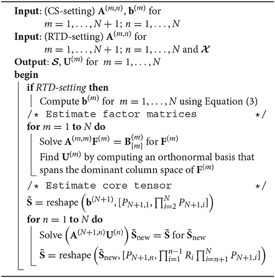
Algorithm 1. MLSVD from a BRKS linear system (lsmlsvd_brks).

2.4. Conditions for MLSVD Retrieval

In this section, we derive the conditions in Theorem 1, under which the retrieval of the MLSVD of ${X}$ from a BRKS system is guaranteed. Since the factor matrices and the core are intrinsic to the data ${X}$, the conditions in this section are to be seen as constraints on the generating matrices.

Theorem 1. Consider a tensor ${X}\in {ℝ}^{I_1\times \cdots \times I_N}$ of multilinear rank (R₁, …, R_N), admitting an MLSVD $⟦{S};{\mathbf{\text{U}}}^{(1)},\dots ,{\mathbf{\text{U}}}^{(N)}⟧$ with factor matrices ${\mathbf{\text{U}}}^{(n)}\in {ℝ}^{I_n\times R_n}$ for n = 1, …, N and core tensor ${S}\in {ℝ}^{R_1\times \cdots \times R_N}$. Given linear combinations b of $\mathrm{\text{vec}}({X})$ obtained from a BRKS linear system with generating matrices ${\mathbf{\text{A}}}^{(m,n)}\in {ℝ}^{P_{mn}\times I_n}$ for m = 1, …, N + 1 and n = 1, …, N, the factor matrices U⁽ⁿ⁾ for n = 1, …, N can be retrieved if and only if

$\begin{array}{ll}1)& \text{r}\left(A^{(m,m)}\right)=I_m\text{for }m=1,\dots ,N;\\ 2)& {\displaystyle \prod _{n\ne m}^N}\text{r}\left({\text{A}}^{(m,n)}{\text{U}}^{(n)}\right)\ge R_m\text{for }m=1,\dots ,N.\end{array}$

The core ${S}$ can be retrieved if and only if

$\begin{array}{l}3){\displaystyle \prod _{n=1}^N}\text{r}\left({\text{A}}^{(N+1,n)}{\text{U}}^{(n)}\right)={\displaystyle \prod _{n=1}^N}{R}_n.\end{array}$

Proof: Condition 1): The linear system in Equation (9) can be uniquely solved for F^(m) if and only if A^(m,m) is of full column rank I_m for m = 1, …, N.

Condition 2): An orthonormal basis of dimension R_m for the column space of F^(m) can be retrieved if and only if

$\begin{array}{l}\text{r}\left({\text{U}}^{(m)}{\text{S}}^{(m)}\right)=\text{r}\left({\text{U}}^{(m)}{\text{S}}_{[m]}\left({\displaystyle \underset{n\ne m}{\otimes }}\left({\text{A}}^{(m,n)}{\text{U}}^{(n)}\right)\right)\right)\\ =R_m\text{for }m=1,\dots ,N\end{array}$

holds. Since $\mathrm{\text{r}}\left({\mathbf{\text{U}}}^{(m)}\right)=\mathrm{\text{r}}({{S}}_{[m]})=R_m$, which follows from the definition of the MLSVD, this condition reduces to

$\begin{array}{l}\text{r}\left({\displaystyle \underset{n\ne m}{\otimes }}\left({\text{A}}^{(m,n)}{\text{U}}^{(n)}\right)\right)={\displaystyle \prod _{n\ne m}^N}\text{r}\left({\text{A}}^{(m,n)}{\text{U}}^{(n)}\right)\\ \ge R_m\text{for }m=1,\dots ,N.\end{array}$

Condition 3): The linear system in Equation (11) can be uniquely solved for $\mathrm{\text{vec}}({S})$ if and only if the coefficient matrix ${\otimes }_{n=1}^N\left({\mathbf{\text{A}}}^{(N+1,n)}{\mathbf{\text{U}}}^{(n)}\right)$ is of full column rank:

$\begin{array}{l}\text{r}\left({\displaystyle \underset{n=1}{\overset{N}{\otimes }}}{\text{A}}^{(N+1,n)}{\text{U}}^{(n)}\right)={\displaystyle \prod _{n=1}^N}\text{r}\left({\text{A}}^{(N+1,n)}{\text{U}}^{(n)}\right)={\displaystyle \prod _{n=1}^N}{R}_n.\end{array}$

The conditions in Theorem 1 are satisfied in the generic case, in which the generating matrices are sampled from a continuous probability distribution and thus are of full rank with probability 1, if and only if the conditions in Theorem 2 hold. The conditions in the latter theorem allow us to determine the dimensions P_mn for m = 1, …, N + 1 and n = 1, …, N of the generating matrices such that generically the MLSVD of ${X}$ can be retrieved.

Theorem 2. With generic generating matrices A^(m,n) for m = 1, …, N + 1 and n = 1, …, N, the conditions in Theorem 1 hold if and only if

$\begin{array}{ll}1)& P_{mm}\ge I_m\text{for }m=1,\dots ,N;\\ 2)& {\displaystyle \prod _{n\ne m}}\text{min}(P_{mn},R_n)\ge R_m\text{for }m=1,\dots ,N;\\ 3)& P_{N+1,n}\ge R_n\text{for }n=1,\dots ,N.\end{array}$

Proof: The proof of these conditions follows from the conditions in Theorem 1 and the properties of generic matrices.

Condition 1): Since a generic matrix is of full rank, $\mathrm{\text{r}}\left({\mathbf{\text{A}}}^{(m,m)}\right)=min(P_{mm},I_m)$ for m = 1, …, N.

Condition 2): The matrix product A^(m,n)U⁽ⁿ⁾ is of full rank min(P_mn, R_n) with probability 1 for a generic matrix A^(m,n) and U⁽ⁿ⁾ of full column rank (the latter following from the definition of an MLSVD) with P_mn, R_n ≤ I_n for m = 1, …, N + 1 and n = 1, …, N [10, Lemma 1].

Condition 3): Similar to the proof of condition 2), generically $\mathrm{\text{r}}\left({\mathbf{\text{A}}}^{(N+1,n)}{\mathbf{\text{U}}}^{(n)}\right)=\mathrm{\text{min}}(P_{N+1,n},R_n)$ for n = 1, …, N according to Sidiropoulos and Kyrillidis [10, Lemma 1]. Condition 3) in Theorem 1 then reduces to ${\prod }_{n=1}^{N}min(P_{N+1,n},R_n)\ge {\prod }_{n=1}^N{R}_n$, which holds if and only if condition 3) in this theorem is satisfied.

In practice, the dimensions P_mn can easily be chosen such that the second generic condition is satisfied with P_mn < R_n for m, n = 1, …, N and n ≠ m. The second condition then reduces to ${\prod }_{n\ne m}^N{P}_{mn}\ge R_m$ for m = 1, …, N. Assuming that P_mn for m = 1, …, N and n ≠ m are approximately equally large, we obtain the condition $P_{mn}\ge \sqrt[N-1]{R_m}$, meaning that the generating matrices ${\mathbf{\text{A}}}^{(m,n)}\in {ℝ}^{P_{mn}\times I_n}$ for m, n = 1, …, N and n ≠ m can be chosen as fat matrices. Therefore, the mth block row of Equation (3) compresses all modes of ${X}$ except the mth, as illustrated in Figure 1, similar to an RTD algorithm for the MLSVD. Additionally, this implies that ${\mathbf{\text{B}}}_{[m]}^{(m)}\in {ℝ}^{P_{mm}\times {\prod }_{n\ne m}{P}_{mn}}$ holds at least R_m columns, which is indeed the minimum required number for estimating the R_m-dimensional mode-m subspace of ${X}$. Algorithm 1 uses an oversampling factor q ≥ 1 such that this matrix holds more than the minimum required number of columns, namely ∏_{n ≠ m} P_mn = qR_m columns for m = 1, …, N. These additional compressed measurements allow a better estimation of the factor matrices if the data is noisy.

FIGURE 1

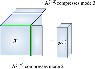
Figure 1. Similar to the RTD algorithm in Che et al. [15], we recover the first MLSVD factor matrix from ${{B}}^{(1)}$, which is a version of ${X}$ that is compressed in every mode except the first.

2.5. Noisy Data

In applications, noise can be present on the compressed measurements and/or on the entries of the tensor. In the former case, the linear system becomes $\mathbf{\text{A}}\mathrm{\text{vec}}({X})=\mathbf{\text{b}}+\mathbf{\text{n}}$, in which the noise vector n is partitioned into subvectors n^(m) for m = 1, …, N, consistent with the partitioning of b in Equation (3). The linear system in Equation (8), with a noise term n, becomes

$\begin{array}{l}{\text{A}}^{(m,m)}{\text{F}}^{(m)}={\text{B}}_{[m]}^{(m)}+{\text{N}}_{[m]}^{(m)}\text{for }m=1,\dots ,N,\end{array}$

in which ${{N}}^{(m)}\in {ℝ}^{P_{m1}\times \cdots \times P_{mN}}$ is the tensor representation of n^(m) and ${\mathbf{\text{N}}}_{[m]}^{(m)}$ its mode-m matrix unfolding. The rank of the matrix, obtained by solving this subsystem for F^(m), generically equals $min\left(I_m,{\prod }_{n\ne m}^N{P}_{mn}\right)$ due to the presence of the noise and thus exceeds R_m if q > 1 for m = 1, …, N. If the signal-to-noise ratio $\frac{\left|\right|\mathbf{\text{b}}|{|}_2}{\left|\right|\mathbf{\text{n}}|{|}_2}$ is sufficiently high, then the dominant column space of F^(m) is nevertheless expected to be a good approximation for the column space of U^(m). A basis for this dominant column space can be computed with the singular value decomposition (SVD) and the approximation is optimal in least squares sense if n^(m) is white Gaussian noise.

In the case of noisy tensor entries, the linear system becomes $\mathbf{\text{A}}\mathrm{\text{vec}}({X}+{N})=\mathbf{\text{b}}$, with ${N}\in {ℝ}^{I_1\times \cdots \times I_N}$. In contrast with the former case, the coefficient matrix now also operates on the noise. Equation (8) then becomes

$\begin{array}{l}{\text{A}}^{(m,m)}\left({\text{F}}^{(m)}+{\text{N}}^{(m)}\right)={\text{B}}_{[m]}^{(m)}\text{with}\\ {\text{N}}^{(m)}={\left({\displaystyle \prod _{n\ne m}}\left({N}{·}_i{\text{A}}^{(m,n)}\right)\right)}_{[m]}\text{for }m=1,\dots ,N.\end{array}$

Because of the noise, the rank of F^(m) + N^(m) generically exceeds R_m for m = 1, …, N. The least squares optimal approximation of the column space of U^(m) can again be retrieved using the SVD if $\left({\otimes }_{n=1}^N{\mathbf{\text{A}}}^{(m,n)}\right)\mathrm{\text{ vec}}({N})$ is white Gaussian noise. As derived in Sidiropoulos et al. [12], this holds true if $\mathrm{\text{vec}}({N})$ is white Gaussian noise and ${\mathbf{\text{A}}}^{(m,n)}{{\mathbf{\text{A}}}^{(m,n)}}^{\mathrm{\text{T}}}={\mathbf{\text{I}}}_{P_{mn}}$ for m, n = 1, …, N. The latter condition is approximately satisfied for large tensor dimensions if the generating matrices are sampled from a zero-mean uncorrelated distribution.

3. Computing an Orthogonally Compressed CPD From a BRKS Linear System

Since the core of the MLSVD of an Nth order tensor is also an Nth order tensor, the MLSVD suffers from the CoD. On the contrary, the number of parameters of the CPD scales linearly with the order of the tensor. Additionally, the CPD is unique under mild conditions. For applications that are more suited to these properties, such as blind signal separation, we introduce an algorithm for computing a CPD from a BRKS linear system in this section. An efficient, three-step approach for computing the CPD of a tensor is: 1) compressing the tensor, 2) decomposing the compressed tensor and 3) expanding the factor matrices to the original dimensions. In Bro and Andersson [9], the tensor is orthogonally compressed using the factor matrices of its MLSVD, i.e., the orthogonally compressed tensor corresponds to the core tensor of the MLSVD. In this section, we generalize this popular approach to computing a CPD from the BRKS linear system in Equation (3). Following this approach, we can find the CPD of a large tensor of order N by computing the CPDs of N small tensors.

3.1. Computing the Factor Matrices

If ${X}$ is approximately of rank R, it admits a CPD

$\begin{array}{ll}{X}=⟦{\text{W}}^{(1)},\dots ,{\text{W}}^{(N)}⟧& (13)\end{array}$

with ${\mathbf{\text{W}}}^{(n)}\in {ℝ}^{I_n\times R}$ for n = 1, …, N. Since the dimension of the subspace spanned by the mode-n vectors of ${X}$ is at most of dimension R for n = 1, …, N, as ${X}$ is of rank R, ${X}$ also admits an MLSVD

$\begin{array}{ll}{X}=⟦{S};{\text{U}}^{(1)},\dots ,{\text{U}}^{(N)}⟧& (14)\end{array}$

with ${\mathbf{\text{U}}}^{(n)}\in {ℝ}^{I_n\times R}$ for n = 1, …, N and ${S}\in {ℝ}^{R\times \cdots \times R}$. Note that the rank R_n of the mode-n vectors of ${X}$ can be smaller than R for any n = 1, …, N, namely when W⁽ⁿ⁾ is not of full column rank. In this case, an orthogonal compression matrix U⁽ⁿ⁾ of dimensions I_n × R_n can still be used. Equation (13) and (14) together imply that the core tensor ${S}$ admits the following CPD:

$\begin{array}{ll}{S}=⟦{{\text{U}}^{(1)}}^{\text{T}}{\text{W}}^{(1)},\dots ,{{\text{U}}^{(N)}}^{\text{T}}{\text{W}}^{(N)}⟧=⟦{\text{V}}^{(1)},\dots ,{\text{V}}^{(N)}⟧.& (15)\end{array}$

Alternatively, the CPD of ${X}$ can be written as

$\begin{array}{l}{X}=⟦{\text{U}}^{(1)}{\text{V}}^{(1)},\dots ,{\text{U}}^{(N)}{\text{V}}^{(N)}⟧\end{array}$

by substituting Equation (15) into Equation (14). This CPD can be substituted for ${S}$ in the BRKS system in Equation (3). Using the mixed product property of the Khatri–Rao product, the mth block row of the BRKS system becomes

$\begin{array}{l}\left({\displaystyle \underset{n=1}{\overset{N}{\odot }}}\left({\text{A}}^{(m,n)}{\text{U}}^{(n)}{\text{V}}^{(n)}\right)\right)1_R={\text{b}}^{(m)}\text{for }m=1,\dots ,N.\end{array}$

Tensorizing this equation yields a polyadic decomposition (PD) expression for each block row of the BRKS system:

$\begin{array}{l}⟦{\text{A}}^{(m,1)}{\text{U}}^{(1)}{\text{V}}^{(1)},\dots ,{\text{A}}^{(m,N)}{\text{U}}^{(N)}{\text{V}}^{(N)}⟧={{B}}^{(m)}\text{for }m=1,\dots ,N.\end{array}$

(Note that, since the number of rank-1 terms in this PD is not necessarily minimal, it is a priori not necessarily canonical. However, we will assume further on that the m-th factor matrix in the PD of ${\tilde{{B}}}^{(m)}$ is unique for m = 1, …, N. As that implies that a decomposition in fewer terms is impossible, the PDs are CPDs by our assumption). After solving Equation (9) for F^(m) and estimating U^(m) for m = 1, …, N as described in Section 2.1, the tensorization ${{F}}^{(m)}\in {ℝ}^{P_{m1}\times \cdots \times I_m\times \cdots \times P_{mN}}$ of F^(m) is orthogonally compressed

$\begin{array}{l}{\tilde{{B}}}^{(m)}={{F}}^{(m)}{·}_m{{\text{U}}^{(m)}}^{\text{T}}\\ =⟦{\text{A}}^{(m,1)}{\text{U}}^{(1)}{\text{V}}^{(1)},\dots ,{\text{V}}^{(m)},\dots ,{\text{A}}^{(m,N)}{\text{U}}^{(N)}{\text{V}}^{(N)}⟧\\ \text{ for }m=1,\dots ,N.& (16)\end{array}$

The CPD of the compressed tensor ${\tilde{{B}}}^{(m)}$ shares the factor matrix V^(m) with the CPD of the core tensor ${S}$. The factor matrices V⁽ⁿ⁾ for n = 1, …, N of the CPD of the core can thus be found by computing the CPD of each compressed tensor if the mth factor matrix of the CPD of ${\tilde{{B}}}^{(m)}$ is unique for m = 1, …, N. If the CPD of the full tensor ${X}$ is also unique, its factor matrices can be retrieved by expanding the factor matrices W⁽ⁿ⁾ = U⁽ⁿ⁾V⁽ⁿ⁾ for n = 1, …, N. Since a CPD can only be unique up to the factor scaling and permutation indeterminacies and each factor matrix V⁽ⁿ⁾ for n = 1, …, N is retrieved from a different compressed tensor, the indeterminacies must be addressed. To this end, the fact that the N tensors ${\tilde{{B}}}^{(m)}$ all have the same CPD, up to the (known) compression matrices A^(m,n) for m, n = 1, …, N, can be exploited.

3.2. Algorithm

The steps in Section 3.1 mimic the popular approach in Bro and Andersson [9] for computing the CPD of a fully given tensor, which is: 1) compute the MLSVD of ${X}$, 2) compute the CPD of the core ${S}$ and 3) expand the factor matrices W⁽ⁿ⁾ = U⁽ⁿ⁾V⁽ⁿ⁾ for n = 1, …, N. The corresponding steps in the approach in this paper are: 1) compute the MLSVD factor matrices U⁽ⁿ⁾ for n = 1, …, N and orthogonally compress the tensors ${{F}}^{(m)}$ for m = 1, …, N, 2) compute the CPD of the compressed tensors and 3) expand the factor matrices W⁽ⁿ⁾ = U⁽ⁿ⁾V⁽ⁿ⁾ for n = 1, …, N. Instead of computing the CPD of a core tensor of dimensions R × ⋯ × R, this approach computes the CPD of the N tensors in Equation (16) which are of dimensions P_m1 × ⋯ × P_m,m−1 × R × P_m,m+1 × ⋯ × P_m,N for m = 1, …, N. As will be shown in Section 3.3, these tensors can be far smaller than the core tensor. Algorithm 2 outlines all steps needed to compute a CPD with orthogonal compression from a BRKS linear system. All steps of this algorithm can be computed in parallel. Like Algorithm 1, Algorithm 2 accomodates both the RTD- and CS-setting.

ALGORITHM 2

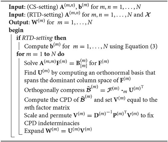
Algorithm 2. Orthogonally compressed CPD from a BRKS linear system (lscpd_brks).

Instead of computing the CPDs of the tensors ${\tilde{{B}}}^{(m)}$ for m = 1, …, N separately, they can also be computed simultaneously as a set of coupled CPDs. These CPDs are coupled since their factor matrices all depend linearly, with coefficients A^(m,n)U⁽ⁿ⁾, on the same factors V⁽ⁿ⁾ for m, n = 1, …, N with n ≠ m. This set of coupled CPDs can be computed in Tensorlab [26] through structured data fusion [27].

3.3. Conditions for CPD Retrieval

In this section, we derive conditions for the identifiability of the CPD of ${X}$ from a BRKS system. The CPD can be identified if the conditions in Theorem 3 hold. In Domanov and De Lathauwer [28], conditions are provided to guarantee that one factor matrix of the CPD is unique.

Theorem 3. Consider a tensor ${X}\in {ℝ}^{I_1\times \cdots \times I_N}$ of rank R, admitting a CPD ${⟦\mathbf{\text{W}}}^{(1)},\dots ,{\mathbf{\text{W}}}^{(N)}⟧$ with factor matrices ${\mathbf{\text{W}}}^{(n)}\in {ℝ}^{I_n\times R}$ for n = 1, …, N. Given linear combinations b of $\mathrm{\text{vec}}({X})$, obtained from a BRKS linear system with generating matrices ${\mathbf{\text{A}}}^{(m,n)}\in {ℝ}^{P_{mn}\times I_n}$ for m, n = 1, …, N, the factor matrices W⁽ⁿ⁾ for n = 1, …, N can be retrieved if

$\begin{array}{ll}1)& \text{r}\left({\text{A}}^{(m,m)}\right)=I_m\text{for }m=1,\dots ,N;\\ 2)& {\displaystyle \prod _{n\ne m}^N}\text{r}\left({\text{A}}^{(m,n)}{\text{U}}^{(n)}\right)\ge R\text{for }m=1,\dots ,N;\\ 3)& \text{The }m\text{th factor matrix of }{\tilde{{B}}}^{(m)}\text{ is unique for }m=1,\dots ,N;\\ 4)& \text{The CPD of }{X}\text{ is unique.}\end{array}$

Proof: Conditions 1) and 2): For the compression matrices U⁽ⁿ⁾ for n = 1, …, N, the factor matrices of the MLSVD of ${X}$ must be retrievable. These conditions are the same as the first two conditions in Theorem 1.

Condition 3): The CPD of the compressed tensor ${\tilde{{B}}}^{(m)}$ for m = 1, …, N in Equation (16) shares the mth factor matrix with the core of the MLSVD of ${X}$ if the mth factor matrix is unique for m = 1, …, N.

Condition 4): While condition 3) ensures that the factor matrices W⁽ⁿ⁾ for n = 1, …, N are unique, condition 4) is needed to ensure that there is only one set of rank-1 tensors, consisting of the columns of W⁽ⁿ⁾ for n = 1, …, N, that forms a CPD of ${X}$, i.e., to exclude different ways of pairing.

In the generic case, in which the generating matrices and the factor matrices of the CPD are sampled from a continuous probability distribution, the CPD of ${X}$ can be identified if the conditions in Theorem 4 hold. Here we used a generic condition to prove the uniqueness of the full CPD of ${\tilde{{B}}}^{(m)}$ for m = 1, …, N, which a fortiori guarantees the uniqueness of its mth factor matrix. The conditions in Theorem 4 can be used to determine the dimensions of the generating matrices that are generically required for the identifiability of the CPD of ${X}$.

Theorem 4. With generic generating matrices A^(m,n) for m,n = 1, …, N, the conditions in Theorem 3 hold if

$\begin{array}{ll}1)& P_{mm}\ge I_m\text{for }m=1,\dots ,N;\\ 2)& {\displaystyle \prod _{n\ne m}^N}\text{min}(P_{mn},R)\ge R\text{for }m=1,\dots ,N;\\ 3)& I_m\ge R\text{for }m=1,\dots ,N;\\ 4)& \{\exists {N}\subset \left\{\left[1,\dots ,N\right]\backslash m\right\}:\text{min}(J_2,J_3)\ge 3\\ & \text{ and }(J_2-1)(J_3-1)\ge R\}\text{for }m=1,\dots ,N\\ & \text{ with }{J}_2={\displaystyle \prod _{n\in {N}}}{P}_{mn}\text{ and }{J}_3={\displaystyle \prod _{n\in {{N}}^c}}{P}_{mn}\end{array}$

Proof: Conditions 1) and 2): These conditions are the same as the first two conditions in Theorem 2.

Condition 3) and 4): The mth factor matrix of ${\tilde{{B}}}^{(m)}$ is unique for m = 1, …, N if the CPD of these tensors is unique. The Nth order tensor ${\tilde{{B}}}^{(m)}$ can be reshaped to a third-order tensor ${Y}\in {ℝ}^{J_1\times J_2\times J_3}$, with J₁ = I_m, $J_2={\prod }_{n\in {N}}{P}_{mn}$, $J_3={\prod }_{n\in {{N}}^c}{P}_{mn}$ and ${N}\subset \left\{[1,\dots ,N]\backslash m\right\}$, of which the first mode corresponds to the uncompressed mth mode of ${\tilde{{B}}}^{(m)}$. The second and third mode, respectively, correspond to a subset ${N}$ of the remaining N − 1 modes and its complementary subset ${{N}}^c$. The rank R CPD of ${\tilde{{B}}}^{(m)}$ is unique if there exists a subset ${N}$ such that the rank R CPD of the reshaped third-order tensor ${Y}$ is unique. Generically, a third-order tensor ${Y}\in {ℝ}^{J_1\times J_2\times J_3}$ of rank R is unique if J₁ ≥ R, min(J₂, J₃) ≥ 3 and (J₂ − 1)(J₃ − 1) ≥ R [29]. Condition 3) guarantees that the former condition is satisfied and condition 4) guarantees that the latter two conditions are satisfied for ${\tilde{{B}}}^{(m)}$ for m = 1, …, N. Additionally, condition 3) guarantees generic uniqueness of the CPD of ${X}$ since for each reshaped, third-order version of ${X}$, all dimensions exceed R [30, Theorem 3].

As explained in Section 2.4, the second condition in Theorem 4 implies that $P_{mn}\ge \sqrt[N-1]{R}$ if the values P_mn are approximately equally large for m, n = 1, …, N and n ≠ m. Similarly, the fourth condition in Theorem 4 implies that

$\begin{array}{l}{P}_{mn}\ge \sqrt[N-1]{{(1+\sqrt{R})}^2}\text{for }m,n=1,\dots ,N\text{ and }n\ne m.\end{array}$

(Note that this bound is derived for tensors of uneven order N. The bound for tensors of even order is similar, but does not have a simple expression). The latter constraint poses only slightly more restrictive bounds than the former, meaning that the dimensions P_mn for m, n = 1, …, N and n ≠ m can still be chosen such that they are much smaller than R. In real applications, tensor dimensions often exceed the tensor rank, satisfying the third condition in Theorem 4.

Remark: Note that the rank of a tensor can exceed some of its dimensions, in which case Theorem 4 cannot be satisfied. This can be resolved by using a different uniqueness condition to guarantee the uniqueness of the CPDs of ${\tilde{{B}}}^{(m)}$ for m = 1, …, N, such as the generic version of Kruskal's condition [31]. However, using this condition also results in stricter bounds on P_mn for m, n = 1, …, N and n ≠ m.

4. Computing a TT From a BRKS Linear System

Since the TT also does not suffer from the CoD, we derive an algorithm for computing a TT from a BRKS linear system in this section. The TT-SVD algorithm in Oseledets [25] computes the cores using sequential SVDs. Unlike in TT-SVD, for a BRKS linear system the SVDs can be computed in parallel by processing the compressed tensors ${{B}}^{(m)}$ for m = 1, …, N of ${X}$ separately.

4.1. Computing the TT Cores

If ${X}$ is approximately of TT-rank (R₀, …, R_N), it admits a TT $⦇{{G}}^{(1)},\dots ,{{G}}^{(N)}⦈$ with cores ${{G}}^{(n)}\in {ℝ}^{R_{n-1}\times I_n\times R_n}$ for n = 1, …, N. Substituting this TT for ${X}$ into the BRKS linear system in Equation (3) leads to

$\begin{array}{l}\text{A}\text{vec}\left(⦇{{G}}^{(1)},\dots ,{{G}}^{(N)}⦈\right)=\text{b}.\end{array}$

It follows that the tensorized mth block row of this BRKS system corresponds to the TT of ${X}$ transformed through mode-n multiplication with the generating matrices A^(m,n):

$\begin{array}{l}{{B}}^{(m)}=⦇{{H}}^{(m,1)},\dots ,{{H}}^{(m,N)}⦈\end{array}$

with ${{H}}^{(m,n)}={{G}}^{(n)}{·}_2{\mathbf{\text{A}}}^{(m,n)}$ for n = 1, …, N. Rearranging this transformed TT into its mode-m unfolding leads to

$\begin{array}{l}{\text{A}}^{(m,m)}{\left(⦇{{H}}^{(m,1)},\dots ,{{H}}^{(m,m-1)},{{G}}^{(m)},{{H}}^{(m,m+1)},\dots ,{{H}}^{(m,N)}⦈\right)}_{[m]}\\ ={\text{B}}_{[m]}^{(m)}.\end{array}$

This unfolding corresponds to a linear system

$\begin{array}{ll}{\text{A}}^{(m,m)}{\tilde{\text{B}}}_{[m]}^{(m)}={\text{B}}_{[m]}^{(m)}& (17)\end{array}$

that can be solved for ${\widetilde{\mathbf{\text{B}}}}_{[m]}^{(m)}$. The tensor ${\tilde{{B}}}^{(m)}$ is a transformed TT of ${X}$ that shares the mth core ${{G}}^{(m)}$ with the TT of the full tensor ${X}$. Following the definition of a TT, this core can be retrieved from the column space of the following matrix unfolding

$\begin{array}{l}{\tilde{\text{B}}}_{[1,\dots ,m;m+1,\dots ,N]}^{(m)}=(⦇{{H}}^{(m,1)},\dots ,{{H}}^{(m,m-1)},{{G}}^{(m)}⦈{)}_{[m+1]}^{\text{T}}\\ {\left(⦇{{H}}^{(m,m+1)},\dots ,{{H}}^{(m,N)}⦈\right)}_{[1]}.& (18)\end{array}$

(W.r.t. the matricization, note that while $⦇{{H}}^{(m,1)},\dots ,{{H}}^{(m,m-1)},{{G}}^{(m)}⦈$ consists of m cores, it is a tensor of order m + 1 since R_m is not necessarily equal to one). First, we retrieve ${{G}}^{(1)}$ by computing an orthonormal basis of dimension R₁ for the dominant column space of the matrix unfolding in Equation (18) for m = 1. For m = 2, …, N, the column space of this unfolding also involves the preceding cores ${{H}}^{(m,1)},\dots ,{{H}}^{(m,m-1)}$. If the cores are computed in order, then these preceding cores are known and can be compensated for by subsequently solving smaller linear systems

$\begin{array}{ll}{\text{H}}_{[1,2;3]}^{(m,n)}{\text{B}}_{\text{new}}^{(n)}={\text{B}}^{(n)}\text{for }n=1,\dots ,m-1,& (19)\end{array}$

for ${\mathbf{\text{B}}}_{\mathrm{\text{new}}}^{(n)}$, with ${\mathbf{\text{B}}}^{(1)}={\widetilde{\mathbf{\text{B}}}}_{[1]}^{(m)}$ and ${\mathbf{\text{B}}}^{(n)}=\mathrm{\text{reshape}}\left({\mathbf{\text{B}}}_{\mathrm{\text{new}}}^{(n-1)},[R_{n-1}{P}_{mn},I_m{\prod }_{k=n+1}^N{P}_{mk}]\right)$ for n = 2, …, m − 1. After solving these systems, ${{G}}^{(m)}$ is retrieved by computing an orthonormal basis of dimension R_m for the dominant column space of $\mathrm{\text{reshape}}\left({\mathbf{\text{B}}}_{\mathrm{\text{new}}}^{(n)},[R_{m-1}{I}_m,{\prod }_{k=m+1}^N{P}_{mk}]\right)$ for m = 1, …, N.

Alternatively, we can immediately compute an orthonormal basis of dimension R_m for the dominant column space of the matrix unfolding in Equation (18) for m = 1, …, N, without compensating for preceding cores first. Computing these bases is more expensive, since they are obtained from a larger matrix than in the case where the preceding cores have already been compensated for. On the other hand, the orthonormal bases can be computed in parallel, as there is no dependency on any preceding core. If after the orthonormal bases have been found, also the cores of the TT are desired, compensation of preceding cores can be done in a similar manner as described above, namely by subsequently solving linear systems. These linear systems have the same coefficient matrix as the linear systems in Equation (19).

4.2. Algorithm

Algorithm 3 outlines all steps needed to compute a TT from a BRKS linear system for the approach in which the orthonormal bases are computed first and the preceding cores are compensated for second. Note that only N − 1 SVDs need to be computed, just like in the standard TT-SVD algorithm, in which the final SVD reveals both cores N − 1 and N. Like Algorithm 1 and 2, Algorithm 3 also accommodates both the RTD- and CS-setting.

ALGORITHM 3

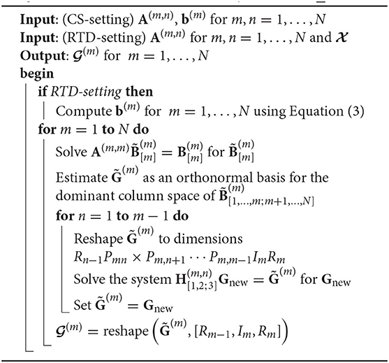
Algorithm 3. TT from a BRKS linear system (lstt_brks).

Remark: When computing the mth core in Algorithm 3, the m − 1 preceding compressed cores ${{H}}^{(m,1)},\dots ,{{H}}^{(m,m-1)}$ in ${\tilde{{B}}}^{(m)}$ are compensated for from left to right, i.e., for m = 1, …, n − 1. If ${\tilde{{B}}}^{(m)}$ is unfolded in reverse, i.e.,

$\begin{array}{l}{\tilde{\text{B}}}_{[N,\dots ,m;m-1,\dots ,1]}^{(m)}=(⦇{{H}}^{(m,N)},\dots ,{{H}}^{(m,m+1)},{{G}}^{(m)}⦈{)}_{[N-m+2]}^{\text{T}}\\ {\left(⦇{{H}}^{(m,m-1)},\dots ,{{H}}^{(m,1)}⦈\right)}_{[1]},& (20)\end{array}$

then the column space of the unfolding contains, besides ${{G}}^{(m)}$, the N − m next compressed cores ${{H}}^{(m,N)},\dots ,{{H}}^{(m,m+1)}$. This way, it is possible to compute the mth core by compensating for these next compressed cores from right to left, i.e., ${{H}}^{(m,N)},\dots ,{{H}}^{(m,m+1)}$. The efficiency of Algorithm 3 can be improved by computing the first half of the cores using the unfolding in Equation (18) and compensating for the preceding cores from left to right, and the second half of the cores using the unfolding in Equation (20) and compensating for the next cores from right to left. This halves the number of cores that need to be compensated for compared to Algorithm 3, in which cores are only compensated for from left to right to simplify the pseudocode.

4.3. Conditions for TT Retrieval

In this section, we derive the conditions in Theorem 5, under which retrieval of the TT of ${X}$ from a BRKS system is guaranteed. The compensation for preceding cores occurs in both approaches for computing the TT in Section 4.1. Therefore, the linear systems that are solved to compensate for them must have a unique solution. Since these linear systems have the same coefficient matrices in both approaches, the condition under which they have a unique solution is the same, regardless of the chosen approach.

Theorem 5. Consider a tensor ${X}\in {ℝ}^{I_1\times \cdots \times I_N}$ of TT-rank (R₀, …, R_N), admitting a TT $⦇{{G}}^{(1)},\dots ,{{G}}^{(N)}⦈$ with cores ${{G}}^{(n)}\in {ℝ}^{R_{n-1}\times I_n\times R_n}$ for n = 1, …, N. Given linear combinations b of $\mathrm{\text{vec}}({X})$, obtained from a BRKS linear system with generating matrices ${\mathbf{\text{A}}}^{(m,n)}\in {ℝ}^{P_{mn}\times I_n}$ for m, n = 1, …, N, the cores ${{G}}^{(n)}$ for n = 1, …, N can be retrieved if and only if

$\begin{array}{l}1)\text{r}\left({\text{A}}^{(m,m)}\right)=I_m\text{for }m=1,\dots ,N;\\ 2)\text{r}\left({\tilde{\text{B}}}_{[1,\dots ,m;m+1,\dots ,N]}^{(m)}\right)=R_m\text{for }m=1,\dots ,N;\\ 3)\text{r}\left({\text{H}}_{[1,2;3]}^{(m,n)}\right)=R_n\text{for }m=1,\dots ,N\text{ and }n=1,\dots ,m-1.\end{array}$

Proof: Condition 1): The linear system in Equation (17) can be uniquely solved for ${\widetilde{\mathbf{\text{B}}}}_{[m]}^{(m)}$ if and only if A^(m,m) is of full column rank I_m for m = 1, …, N.

Condition 2): An orthonormal basis of dimension R_m for the column space of the matricization ${\widetilde{\mathbf{\text{B}}}}_{[1,\dots ,m;m+1,\dots ,N]}^{(m)}$ in Equation (18) can be retrieved if and only if the rank of this matricization equals R_m.

Condition 3): The linear systems that are solved to compensate for compressed cores have a unique solution if and only if

$\begin{array}{l}\text{r}\left({\text{H}}_{[1,2;3]}^{(m,n)}\right)=R_n\text{for }m=1,\dots ,N\text{ and }n=1,\dots ,m-1\end{array}$

holds.

In the generic case, in which the generating matrices are sampled from a continuous probability distribution, the TT of ${X}$ can be retrieved if the conditions in Theorem 6 hold. These conditions can be used to determine the dimensions of the generating matrices such that the TT of ${X}$ can generically be retrieved.

Theorem 6. With generic generating matrices A^(m,n) for m, n = 1, …, N, the conditions in Theorem 1 hold if and only if

$\begin{array}{l}1)P_{mm}\ge I_m\text{for }m=1,\dots ,N;\\ 2)P_{mn}\ge \frac{R_m}{R_{n-1}{I}_m{\displaystyle {\prod }_{k=n+1}^{m-1}}{P}_{mk}}\\ \text{ for }m=1,\dots ,N\text{ and }n=1,\dots ,n-1;\\ 3)P_{mn}\ge \frac{R_m}{R_n{\displaystyle {\prod }_{k=m+1}^{n-1}}{P}_{mk}}\\ \text{ for }m=1,\dots ,N\text{ and }n=m+1,\dots ,N;\\ 4)P_{mn}\ge \frac{R_n}{R_{n-1}}\text{for }m=1,\dots ,N\text{ and }n=1,\dots ,m-1.\end{array}$

Proof: Condition 1): This condition is the same as condition 1) in Theorem 2.

Condition 2): The matricization ${\widetilde{\mathbf{\text{B}}}}_{[1,\dots ,m;m+1,\dots ,N]}^{(m)}$ in Equation (18) equals

$\begin{array}{l}{\tilde{\text{B}}}_{[1,\dots ,m;m+1,\dots ,N]}^{(m)}=\\ ({\text{G}}_{[3]}^{(m)}({\text{H}}_{[3]}^{(m,m-1)}(\cdots {\text{H}}_{[3]}^{(m,2)}({\text{H}}_{[3]}^{(m,1)}\otimes {\text{I}}_{P_{m2}})\cdots \otimes {\text{I}}_{P_{m,m-1}})\otimes {\text{I}}_{I_m}){)}^{\text{T}}\\ \left({\text{H}}_{[1]}^{(m,m+1)}\left({\text{I}}_{P_{m,m+1}}\otimes \cdots {\text{H}}_{[1]}^{(m,N-1)}\left({\text{I}}_{P_{m,N-1}}\otimes {\text{H}}_{[1]}^{(m,N)}\right)\right)\right)=:{\text{D}}^{\text{T}}\text{E}.& (21)\end{array}$

Generically, the rank of ${\widetilde{\mathbf{\text{B}}}}_{[1,\dots ,m;m+1,\dots ,N]}^{(m)}$ equals R_m if and only if the rank of both D and E equals R_m. Condition 2) relates to D and condition 3) to E. Since ${\mathbf{\text{G}}}_{[3]}^{(m)}$ is of full rank, which follows from the definition of a TT, and ${\mathbf{\text{H}}}_{[3]}^{(m,n)}$ for n ≠ m is generically of full rank, each matrix product in Equation (21) is also of full rank [10, Lemma 1]. Therefore, the rank of D generically equals

$\begin{array}{l}min(\text{r}\left({\displaystyle {\text{G}}_{[3]}^{(m)}}\right),min(\text{r}\left({\displaystyle {\text{H}}_{[3]}^{(m,m-1)}}\right),\dots ,\\ min\left(\text{r}\left({\displaystyle {\text{H}}_{[3]}^{(m,2)}}\right),\text{r}\left({\text{H}}_{[3]}^{(m,1)}\right)P_{m2})P_{m3}\cdots P_{m,m-1}\right)I_m).\end{array}$

Both arguments of the leftmost min(·) must at least equal R_m such that r (D) ≥ R_m holds. Following the definition of a TT, this always holds true for the first argument $\mathrm{\text{r}}\left({\mathbf{\text{G}}}_{[3]}^{(m)}\right)$. The second argument is min(·)I_m, so both arguments of this second min(·) must at least equal $\frac{R_m}{I_m}$. Generically $\mathrm{\text{r}}\left({\mathbf{\text{H}}}_{[3]}^{(m,m-1)}\right)=min(P_{m,m-1}{R}_{m-2},R_{m-1})$, leading to the conditions $P_{m,m-1}\ge \frac{R_m}{R_{m-2}{I}_m}$ and R_m−1I_m ≥ R_m. The latter condition is satisfied by the definition of a TT. Repeating the same steps for each subsequent min(·) leads to the conditions

$\begin{array}{l}{P}_{mn}\ge \frac{R_m}{R_{n-1}{I}_m{\displaystyle {\prod }_{k=n+1}^{m-1}}{P}_{mk}}\\ \text{ for }m=1,\dots ,N\text{ and }n=1,\dots ,m-1.\end{array}$

Condition 3): In a similar fashion, it can be proven that r (E) ≥ R_m holds if and only if

$\begin{array}{l}{P}_{mn}\ge \frac{R_m}{R_n{\displaystyle {\prod }_{k=m+1}^{n-1}}{P}_{mk}}\text{for }m=1,\dots ,N\text{ and }n=m+1,\dots ,N.\end{array}$

Condition 4): Since a generic matrix is of full rank, $\mathrm{\text{r}}\left({\mathbf{\text{H}}}_{[1,2;3]}^{(m,n)}\right)=\mathrm{\text{min}}(R_{n-1}{P}_{mn},R_n)$ for m, n = 1, …, N.

5. Experiments

In this section, we validate our algorithms using synthetic and real data. The algorithms are implemented in MATLAB and are available at https://www.tensorlabplus.net. In the practical implementation of the algorithms, column spaces are estimated using the SVD and linear systems are solved using the MATLAB backslash operator. All experiments are performed on a laptop with an AMD Ryzen 7 PRO 3700U processor and 32GB RAM. The algorithms are run sequentially even though each algorithm can (partly) be executed in parallel.

Since it is possible to choose the generating matrices in the experiments in this section, we set A_mm = I_Im for m = 1, …, N. This means that the first step in each algorithm, namely solving a linear system with A_mm as the coefficient matrix, can be skipped. First, we use synthetic data to compare the accuracy and computation time of these algorithms to related algorithms. All synthetic problems are constructed by sampling the entries of the factor matrices and/or core(s) of a tensor decomposition from the standard normal distribution. Additive Gaussian noise ${N}$ is added to these randomly generated tensors ${X}$ and the noise level is quantified using the signal-to-noise ratio (SNR):

$\begin{array}{l}\text{SNR}=10{log}_{10}\left(\frac{\left|\right|{X}|{|}_{\text{F}}^2}{\left|\right|{N}|{|}_{\text{F}}^2}\right).\end{array}$

5.1. Randomized MLSVD

In the first experiment, a random third-order tensor ${X}\in {ℝ}^{I\times I\times I}$ of low multilinear rank (R, R, R), with I = 200 and R = 10, is generated with varying levels of noise. The factor matrices of the MLSVD of ${X}$ are then retrieved from a BRKS linear system using Algorithm 1. The entries of the generating matrices are sampled from the standard normal distribution. This means that we are using Algorithm 1 in the RTD-setting in this experiment. The dimensions of the generating matrices are determined using the oversampling factor q = 5 and the multilinear rank of ${X}$. For this value of q, the sampling ratio equals 0.005. This ratio is defined as the number of compressed measurements in b divided by the number of entries in ${X}$. We compare the accuracy of our algorithm with related RTD algorithms and a cross-approximation algorithm for low multilinear rank approximation. These algorithms are:

• rand_tucker Algorithm 2 in [16]: The factor matrices U⁽ⁿ⁾ for n = 1, …, N are retrieved as follows: 1) the mode-n matrix unfolding of ${X}$ is compressed through multiplication with a random Gaussian matrix and 2) an orthonormal basis for this compressed matrix unfolding is computed using the QR decomposition. After computing each factor matrix, ${X}$ is orthogonally compressed using this factor matrix like in the sequentially truncated higher-order SVD algorithm [32]. The oversampling factor is set to p = 5, which means that this algorithm actually estimates an MLSVD of multilinear rank (R + p, R + p, R + p).

• rand_tucker_kron algorithm 4.2 in [15]: Similar to rand_tucker, but the algorithm uses a Kronecker-structured matrix for compression and the SVD for computing an orthonormal basis. The oversampling factor for this algorithm is chosen such that it is the same as our oversampling factor q in Section 2.4.

• mlsvd_rsi [33]: Computes an MLSVD using sequential truncation [32] and uses randomized compression and subspace iteration for estimating the SVD [34]. In the randomized compression step, the mode-n unfolding X_[n] is compressed through matrix multiplication with a random matrix of dimensions ∏_{i ≠ n}I_i × R_n + p, with an oversampling factor p = 5. Next, the nth factor matrix is estimated by computing an SVD of this randomly compressed matrix and further refined using two subspace iteration steps with the full mode-n unfolding X_[n].

• lmlra_aca [21]: Cross approximation approach for low multilinear rank approximation.

The last two algorithms are available in Tensorlab [26]. As the full tensor ${X}$ is usually available in the RTD-setting, the core is computed as

$\begin{array}{l}{S}={X}{·}_1{{\text{U}}^{(1)}}^{\text{T}}\cdots {·}_N{{\text{U}}^{(N)}}^{\text{T}}.\end{array}$

Figure 2 compares the accuracy, quantified as a relative error

$\begin{array}{l}{E}_{\text{rel}}=\frac{||{X}-\widehat{{S}}{·}_1{\widehat{\text{U}}}^{(1)}\cdots {·}_N{\widehat{\text{U}}}^{(N)}|{|}_{\text{F}}}{||{X}|{|}_{\text{F}}}\end{array}$

with $\widehat{{S}}$ and ${\widehat{\mathbf{\text{U}}}}^{(n)}$ for n = 1, …, N the estimated core and factor matrices, of these algorithms. The error shown in Figure 2 is the average relative error over 10 trials. Algorithm lsmlsvd_brks is more accurate than rand_tucker and lmlra_aca. Algorithm mlsvd_rsi is far more accurate than all other algorithms because it uses subspace iteration with the full mode-n matrix unfolding of ${X}$ for computing the nth factor matrix. For this reason it also has the longest computation time of all algorithms. Algorithm rand_tucker_kron is more accurate than lsmlsvd_brks due to the sequential truncation step in rand_tucker_kron after each factor matrix is computed. If this step is omitted, which corresponds to Che et al. algorithm 4.1 in [15], it achieves the same accuracy as lsmlsvd_brks. This sequential truncation step is not possible in lsmlsvd_brks since this algorithm only uses the compressed measurements b instead of the full tensor ${X}$. Note that increasing the oversampling factors of the algorithms results in higher accuracy in exchange for a longer computation time and requiring more compressed datapoints.

FIGURE 2

Figure 2. Algorithm mlsvd_rsi is by far the most accurate because it used the full-sized matrix unfolding in the subspace iteration step. Algorithm lsmlsvd_brks is more accurate than lmlra_aca and rand_tucker and less accurate than rand_tucker_kron. If the sequential truncation step in rand_tucker_kron is omitted, it achieves the same accuracy as lsmlsvd_brks.

5.2. Randomized CPD

In this experiment, we generate a CPD with random factor matrices of a third-order tensor ${X}\in {ℝ}^{I\times I\times I}$, with I = 100, of rank R = 10. Varying levels of noise are added to this tensor. Algorithm 2 is used in the RTD-setting to estimate the factor matrices of the CPD of ${X}$. To compute the CPDs of the compressed tensors, we use the cpd function in Tensorlab [26]. This function initializes the factor matrices with a generalized eigenvalue decomposition if possible and further improves them using (second-order) optimization algorithms. The accuracy of the factor matrices estimated by this algorithm are compared to results obtained with related RTD algorithms:

• cpd_rbs [35]: In each iteration, a random subtensor of ${X}$ is sampled and the corresponding rows of the factor matrices are updated. These updates are computed using a Gauss–Newton algorithm. In this experiment, the algorithm starts with random initial factor matrices.

• cp_arls [14]: Alternating least squares with random sketching for solving the least squares subproblems.

The accuracy of the estimated factor matrices is quantified as a relative error

$\begin{array}{l}{E}_{\text{CPD}}={\displaystyle \underset{n}{max}}\frac{||{\widehat{\text{U}}}^{(n)}-{\text{U}}^{(n)}|{|}_{\text{F}}}{||{\text{U}}^{(n)}|{|}_{\text{F}}},\end{array}$

in which the scaling and permutation ambiguities between the true U⁽ⁿ⁾ and estimated ${\widehat{\mathbf{\text{U}}}}^{(n)}$ factor matrix have been resolved for n = 1, …, N. Figure 3 shows the average relative error on the left and the average computation time for tensors with increasing dimensions on the right. Both averages are computed over 10 trials. For lscpd_brks, sampling the randomly compressed tensors, i.e., evaluating Equation (3), is included in the computation time. The oversampling factor q of lscpd_brks is set to 5, 10 or 50. For a larger value of q, U⁽ⁿ⁾ better captures the mode-n subspace of ${X}$ and less information is lost during the orthogonal compression step. Figure 3 illustrates that the algorithm is much more accurate for q = 50, while the increase in computation time compared to q = 5 is negligible. If q is set such that the size of the compressed tensors in Equation (4) is of the same order as the full tensor ${X}$, then the computation time will of course increase significantly. For q = 50, the number of compressed datapoints in b equals just 15% of the total number of datapoints in ${X}$. This sampling ratio can be even lower for tensors with order greater than three. Algorithm cp_arls is slightly more accurate than lscpd_brks with q = 50 while being much slower in terms of computation time. Algorithm cpd_rbs is even more accurate and is situated in between lscpd_brks and cp_arls for smaller values of I. The computation time of lscpd_brksis dominated by sampling the randomly compressed tensors, since computing the CPD of these small tensors is very fast. Therefore, the computation time of cpd_rbs scales better for higher values of I since sampling random subtensors of ${X}$ is less time consuming than the random compression of ${X}$ in lsmlsvd_brks, which requires multiple large matrix products. In contrast to lscpd_brks, which uses a fixed amount of compressed datapoints determined by the size of the problem and the oversampling factor, cpd_rbs and cp_arls continue randomly sampling from ${X}$ every iteration until a stopping criterion is met.

FIGURE 3

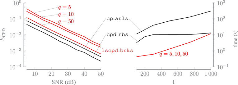
Figure 3. Increasing the oversampling factor q of lscpd_brks, for which the value is shown in the figure, greatly improves its accuracy while having a negligible effect on the computation time. Algorithm lscpd_brks is faster than cp_arls and cp_rbs, for a range of tensor dimensions that are relevant for applications, with a limited loss of accuracy.

5.3. Randomized TT

In this experiment, we generate a TT with random core tensors of a third-order tensor ${X}\in {ℝ}^{I\times I\times I}$, with I = 500, of TT-rank (1, 10, 10, 1). We add varying levels of noise to this tensor and estimate the cores using Algorithm 3 in the RTD-setting. For this experiment, we use the version of this algorithm that first computes orthonormal bases and then compensates for preceding cores. Additionally, preceding cores are compensated for from left to right for the first half of the cores and from right to left for the second half, as explained in Section 4.2. The dimensions of the generating matrices are chosen such that the sampling ratio equals 0.005.

The results of lstt_brks are compared with the results of a related RTD algorithm and a TT cross-approximation approach:

• rand_tt Algorithm 5.1 in [36]: This algorithm is a randomized version of the standard TT-SVD algorithm. The TT-SVD algorithm consists of three steps that are performed for the first N − 1 cores: 1) tensor ${X}$ is matricized, 2) a core is estimated by computing a basis for the column space of this matricization using the SVD and 3) tensor ${X}$ is compressed using this basis. In rand_tt, the matricization in the first step is compressed by multiplying it with a random matrix from the right in order to speed up the computation of the SVD in the next step.

• cross_tt [37]: This algorithm reduces the size of the matricizations of ${X}$ using a maximal volume cross-approximation approach. The matricizations used in this algorithm allow the TT-ranks to be determined adaptively.

The accuracy of the results of these algorithms are quantified as a relative error

$\begin{array}{l}{E}_{\text{rel}}=\frac{||{X}-⦇{\widehat{{G}}}^{(1)},\dots ,{\widehat{{G}}}^{(N)}⦈|{|}_{\text{F}}}{||{X}|{|}_{\text{F}}},\end{array}$

in which ${\widehat{{G}}}^{(n)}$ for n = 1, …, N are the estimated cores. Figure 4 shows the relative error, averaged over 50 trials, and the computation time, averaged over 10 trials, for all algorithms. Tensors of increasing size are used to estimate the computation time. The relative errors achieved by the algorithms with these tensors are in proportion with the errors shown in Figure 4. The relative error is approximately the same for both rand_tt and lstt_brks. The former is faster thanks to the compression step that is performed after computing each core, which causes the tensor to get progressively smaller as the algorithm progresses. However, this algorithm requires the full tensor to be available, whereas the latter works with a limited amount of Kronecker-structured linear combinations of the entries of ${X}$. Therefore, lstt_brks enables us to achieve accuracy comparable to rand_tt in CS applications. If a method for obtaining any entry of ${X}$ is available, then cross_tt can be used to recover a more accurate approximation of the tensor, in exchange for a longer computation time. However, this algorithm is not applicable in the CS-setting either.

FIGURE 4

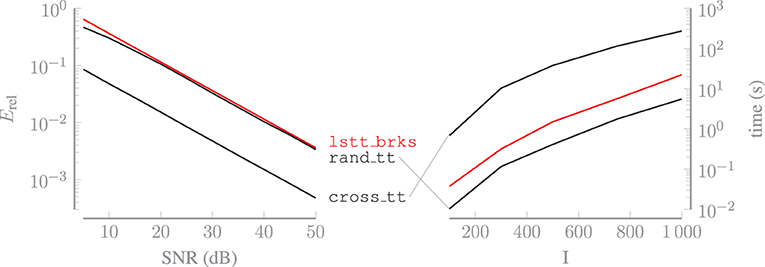
Figure 4. Algorithm lstt_brks enables us to achieve accuracy similar to that of rand_tt in CS applications. If a method for obtaining any entry of ${X}$ is available, then cross_tt can be used to recover a more accurate approximation of the tensor, in exchange for a longer computation time.

5.4. Compressed Sensing Hyperspectral Imaging

In the RTD-setting, the tensor is fully acquired first and then randomly compressed. In the CS-setting, the data can in some applications be compressed during the data acquisition step. For example in hyperspectral imaging, compressed measurements can be obtained using the single-pixel camera [38] or the coded aperture snapshot spectral imager (CASSI) [39]. A hyperspectral image is a third-order tensor ${X}\in {ℝ}^{I_1\times I_2\times I_3}$, consisting of images of I₁ by I₂ pixels taken at I₃ different wavelengths. The single-pixel camera randomly compresses the spatial dimensions of a hyperspectral image. In CASSI, a mask is applied to each I₁ by I₂ image for different wavelengths and these masked images are then aggregated into a single one, i.e., a snapshot. In general, compressed measurements are often obtained in (hyperspectral) imaging by compressing along each dimension separately, meaning that the measurement matrix is Kronecker-structured [11, 40]. With a small number of compressed measurements, a large hyperspectral image can often be accurately reconstructed. Whereas, the random compression step dominated the computation time of our algorithms in the previous experiments, it is missing altogether in this experiment since it is inherent to the application. Therefore, our algorithms enable fast reconstruction of hyperspectral images.

We use lsmlsvd_brks to reconstruct a hyperspectral image using compressed measurements sampled at different sampling ratios. Similar to KCS, this approach expresses ${X}$ in a Kronecker-structured basis, namely the Kronecker product of U⁽ⁿ⁾ for n = 1, 2, 3, in which the core tensor ${S}$ contains the coefficients. In KCS, the bases are chosen a priori such that these coefficients are sparse, which is not necessarily true for the core of an MLSVD. Also, in lsmlsvd_brks, the bases do not have to be chosen a priori as this algorithm also estimates them using compressed measurements. Additionally, in KCS the measurement matrix is Kronecker-structured, whereas it consists of multiple Kronecker-structured block rows in our approach.

Instead of using just the final, (N + 1)th block row of the BRKS system to estimate the core, it makes more sense to use all available compressed measurements to improve the quality of the estimation, since the number of measurements is limited. Therefore, we solve the full BRKS system, with all N + 1 block rows, for a sparse $\mathrm{\text{vec}}({S})$ by optimizing:

$\begin{array}{l}{\displaystyle \underset{\text{vec}({S})}{min}}||\text{vec}({S})|{|}_1\text{subject to }||\text{A}\text{vec}({S})-b|{|}_2\le \sigma .\end{array}$

This is a basis pursuit denoising problem, which can be solved using the SPGL1 solver [41, 42]. The reason for imposing sparsity is as follows. If we were to estimate a dense core tensor using lsmlsvd_brks in this experiment, the number of compressed measurements b^(N+1) certainly cannot be less than the number of entries in the core if we want to be able to retrieve it. However, it turns out that the mode-n vectors of the hyperspectral imaging data ${X}$ cannot be well approximated as linear combinations of a small number of multilinear singular vectors, indicating that the multilinear rank is not small. Estimating a dense core tensor would then require a large number of measurements. On the other hand, it also turns out that in this data only a relatively small number of the entries in a relatively large core is important. We exploit this by computing a sparse approximation of the core, which results in reconstructions of better quality than with the dense core approach, while requiring far less compressed measurements.

The reconstruction results of our algorithm are compared with two other approaches for reconstructing a hyperspectral image from compressed measurements:

• GAP_TV [43]: A generalized alternating projection algorithm that solves the total variation minimization problem. Minimizing total variation leads to accurate image reconstruction because images are generally locally self-similar.

• KCS [11]: We used a two-dimensional Daubechies wavelet basis to sparsify the spatial dimensions and the Fourier basis for the spectral dimension. The sparse coefficients are computed using the SPGL1 solver.

The quality of the reconstructed images is quantified using the peak signal-to-noise ratio (PSNR)

$\begin{array}{l}\text{PSNR}={log}_{10}\left(\frac{max({X})}{\sqrt{\frac{1}{I_1{I}_2{I}_3}||{X}-\widehat{{X}}|{|}_{\text{F}}}}\right),\end{array}$

in which $\widehat{{X}}$ is the reconstructed hyperspectral image. In this experiment, we used the corrected Indian Pines dataset, in which some very noisy wavelengths have been left out [44]. This results in a hyperspectral image of dimensions 145 × 145 × 200. For lsmlsvd_brks, we compute an MLSVD of multilinear rank (70, 70, 30) with a sparse core. This multilinear rank was obtained by trying a wide range of multilinear ranks and assessing the quality of their corresponding reconstructions.

Table 1 shows the quality of the reconstructed images for a range of sampling ratios. Whereas, GAP_TV is specifically designed for imaging applications, lsmlsvd_brks can be applied to a wide range of problems. Regardless, lsmlsvd_brks performs approximately equally well in terms of reconstruction quality. The reconstruction quality achieved by lsmlsvd_brks is higher than for KCS, indicating that the bases estimated by the former suit the data better than the a priori determined bases used in the latter.

TABLE 1

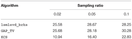
Table 1. This table shows the reconstruction quality, quantified in PSNR (dB), of a hyperspectral image for a range of sampling ratios, obtained with different algorithms. Algorithm lsmlsvd_brks performs approximately equally well as GAP_TV, which is an algorithm specifically suited for image reconstruction. The lower reconstruction quality for KCS indicates that the bases estimated by lsmlsvd_brks suit the data better than the a priori determined bases used in KCS.

6. Conclusion and Further Work

In this work, we have considered a general framework of BRKS linear systems with a compact solution, which suits a wide variety of problems. We developed efficient algorithms for computing an MLSVD, CPD or TT constrained solution from a BRKS system, allowing the user to choose the decomposition that best matches their specific application. The efficiency of these algorithms is enabled on one hand by the BRKS linear system, since such a system produces multiple compressed versions of the tensor and thus splits the problem into a number of smaller ones, and on the other hand by the low (multilinear-/TT-)rank constrained solution. With these algorithms, real data can be accurately reconstructed using far fewer compressed measurements than the total number of entries in the dataset. We have derived conditions under which an MLSVD, CPD or TT can be retrieved from a BRKS system. The corresponding generic versions of these conditions allow us to choose the dimensions of the generating matrices such that a solution can generically be found. Through numerical experiments, we have shown that these algorithms can be used for computing tensor decompositions in a randomized approach. In the case of the CPD, our algorithm needs less computation time than the alternative algorithms. Additionally, we have illustrated the good performance of the algorithms for reconstructing compressed hyperspectral images, despite not being specifically developed for this application. In further work, we will look into parallel implementations for the algorithms in this paper.

Data Availability Statement

Publicly available datasets were analyzed in this study. This data can be found at: https://rslab.ut.ac.ir/data.

Author Contributions

SH derived the algorithms and theory and implemented the algorithms in Matlab. LDL conceived the main idea and supervised the research. Both authors contributed to the article and approved the submitted version.

Funding

This research received funding from the Flemish Government (AI Research Program). LDL and SH are affiliated to Leuven.AI - KU Leuven institute for AI, B-3000, Leuven, Belgium. This work was supported by the Fonds de la Recherche Scientifique–FNRS and the Fonds Wetenschappelijk Onderzoek- Vlaanderen under EOS Project no G0F6718N (SeLMA). KU Leuven Internal Funds: C16/15/059, IDN/19/014.

Conflict of Interest

The authors declare that the research was conducted in the absence of any commercial or financial relationships that could be construed as a potential conflict of interest.

Publisher's Note

All claims expressed in this article are solely those of the authors and do not necessarily represent those of their affiliated organizations, or those of the publisher, the editors and the reviewers. Any product that may be evaluated in this article, or claim that may be made by its manufacturer, is not guaranteed or endorsed by the publisher.

Acknowledgments

The authors would like to thank N. Vervliet and M. Ayvaz for proofreading the manuscript and E. Evert for his help with the mathematical proofs.

Footnotes

1. ^In this context, rank pertains to the definition of rank that corresponds to the respective tensor decomposition.

References

1. Candès EJ, Wakin MB. An introduction to compressive sampling. IEEE Signal Process Mag. (2008). 25:21–30. doi: 10.1109/MSP.2007.914731

CrossRef Full Text | Google Scholar

2. Donoho DL. Compressed sensing. IEEE Trans Inf Theory. (2006) 52:1289–306. doi: 10.1109/TIT.2006.871582

CrossRef Full Text | Google Scholar

3. Ahmadi-Asl S, Abukhovich S, Asante-Mensah MG, Cichocki A, Phan AH, Tanaka T, et al. Randomized algorithms for computation of tucker decomposition and higher order SVD (HOSVD). IEEE Access. (2021) 9:28684–706. doi: 10.1109/ACCESS.2021.3058103

CrossRef Full Text | Google Scholar

4. Acar E, Dunlavy DM, Kolda TG, Morup M. Scalable tensor factorizations for incomplete data. Chemometr Intell Lab. (2011) 3106:41–56. doi: 10.1016/j.chemolab.2010.08.004

CrossRef Full Text | Google Scholar

5. Aldroubi A, Gröchenig K. Nonuniform sampling and reconstruction in shift-invariant spaces. SIAM Rev. (2001) 43:585–620. doi: 10.1137/S0036144501386986

PubMed Abstract | CrossRef Full Text | Google Scholar

6. Oseledets I, Tyrtyshnikov E. TT-cross approximation for multidimensional arrays. Linear Algebra Appl. (2010) 432:70–88. doi: 10.1016/j.laa.2009.07.024

CrossRef Full Text | Google Scholar

7. Udell M, Townsend A. Why are big data matrices approximately low rank? SIAM J Math Data Sci. (2019) 1:144–60. doi: 10.1137/18M1183480

CrossRef Full Text | Google Scholar

8. Rubinstein R, Bruckstein AM, Elad M. Dictionaries for sparse representation modeling. Proc IEEE. (2010) 98:1045–57. doi: 10.1109/JPROC.2010.2040551

CrossRef Full Text | Google Scholar

9. Bro R, Andersson C. Improving the speed of multiway algorithms: part II: compression. Chemometr Intell Lab Syst. (1998) 42:105–13. doi: 10.1016/S0169-7439(98)00011-2

CrossRef Full Text | Google Scholar

10. Sidiropoulos ND, Kyrillidis A. Multi-way compressed sensing for sparse low-rank tensors. IEEE Signal Process. Lett. (2012) 19:757–60. doi: 10.1109/LSP.2012.2210872

CrossRef Full Text | Google Scholar

11. Duarte MF, Baraniuk RG. Kronecker compressive sensing. IEEE Trans Image Process. (2012) 21:494–504. doi: 10.1109/TIP.2011.2165289

PubMed Abstract | CrossRef Full Text | Google Scholar

12. Sidiropoulos N, Papalexakis EE, Faloutsos C. Parallel randomly compressed cubes: a scalable distributed architecture for big tensor decomposition. IEEE Signal Process Mag. (2014) 31:57–70. doi: 10.1109/MSP.2014.2329196

CrossRef Full Text | Google Scholar

13. Kressner D, Tobler C. Low-rank tensor krylov subspace methods for parametrized linear systems. SIAM J Matrix Anal Appl. (2011). 32:1288–316. doi: 10.1137/100799010

CrossRef Full Text | Google Scholar

14. Battaglino C, Ballard G, Kolda TG. A practical randomized CP tensor decomposition. SIAM J Matrix Anal Appl. (2018) 39:876–901. doi: 10.1137/17M1112303

CrossRef Full Text | Google Scholar

15. Che M, Wei Y, Yan H. Randomized algorithms for the low multilinear rank approximations of tensors. J Computat Appl Math. (2021) 390:113380. doi: 10.1016/j.cam.2020.113380

CrossRef Full Text | Google Scholar

16. Zhou G, Cichocki A, Xie S. Decomposition of big tensors with low multilinear rank. (2014) CoRR. abs/1412.1885.

Google Scholar

17. Yang B, Zamzam A, Sidiropoulos ND. ParaSketch: parallel tensor factorization via sketching. In: Proceedings of the 2018 SIAM International Conference on Data Mining (SDM). (2018). p. 396–404.

Google Scholar

18. Jin R, Kolda TG, Ward R. Faster johnson–lindenstrauss transforms via kronecker products. Inf Inference. (2020) 10:1533–62. doi: 10.1093/imaiai/iaaa028

CrossRef Full Text | Google Scholar

19. Mahoney MW, Maggioni M, Drineas P. Tensor-CUR decompositions for tensor-based data. SIAM J Matrix Anal Appl. (2008). 30:957–87. doi: 10.1137/060665336

CrossRef Full Text | Google Scholar

20. Oseledets I, Savostianov DV, Tyrtyshnikov E. Tucker dimensionality reduction of three-dimensional arrays in linear time. SIAM J Matrix Anal Appl. (2008) 30:939–56. doi: 10.1137/060655894

CrossRef Full Text | Google Scholar

21. Caiafa CF, Cichocki A. Generalizing the column-row matrix decomposition to multi-way arrays. Linear Algebra Appl. (2010) 433:557–73. doi: 10.1016/j.laa.2010.03.020

CrossRef Full Text | Google Scholar

22. Goreinov SA, Tyrtyshnikov EE, Zamarashkin NL. A theory of pseudoskeleton approximations. Linear Algebra Appl. (1997) 261:1–21. doi: 10.1016/S0024-3795(96)00301-1

CrossRef Full Text | Google Scholar

23. Kolda TG. Multilinear Operators for Higher-Order Decompositions. Albuquerque, NM; Livermore, CA: Sandia National Laboratories (2006).

Google Scholar

24. De Lathauwer L, De Moor B, Vandewalle J. A multilinear singular value decomposition. SIAM J Matrix Anal Appl. (2000) 21:1253–78. doi: 10.1137/S0895479896305696

CrossRef Full Text | Google Scholar

25. Oseledets I. Tensor-train decomposition. SIAM J Sci Comput. (2011) 33:2295–317. doi: 10.1137/090752286

CrossRef Full Text | Google Scholar

26. Vervliet N, Debals O, Sorber L, Van Barel M, De Lathauwer L. Tensorlab 3.0. (2016). Available online at: https://www.tensorlab.net.

Google Scholar

27. Sorber L, Van Barel M, De Lathauwer L. Structured data fusion. IEEE J Select Top Signal Process. (2015) 9:586–600. doi: 10.1109/JSTSP.2015.2400415

CrossRef Full Text | Google Scholar

28. Domanov I, De Lathauwer L. On the uniqueness of the canonical polyadic decomposition of third-order tensors- Part I: Basic results and uniqueness of one factor matrix. SIAM J Matrix Anal Appl. (2013) 34:855–75. doi: 10.1137/120877234

CrossRef Full Text | Google Scholar

29. Chiantini L, Ottaviani G. On generic identifiability of 3-tensors of small rank. SIAM J Matrix Anal Appl. (2012) 33:1018–37. doi: 10.1137/110829180

CrossRef Full Text | Google Scholar

30. Sidiropoulos N, De Lathauwer L, Fu X, Huang K, Papalexakis EE, Faloutsos C. Tensor decomposition for signal processing and machine learning. IEEE Trans Signal Process. (2017) 65:3551–82. doi: 10.1109/TSP.2017.2690524

CrossRef Full Text | Google Scholar

31. Kruskal JB. Three-way arrays: rank and uniqueness of trilinear decompositions, with application to arithmetic complexity and statistics. Linear Algebra Appl. (1977) 18:95–138. doi: 10.1016/0024-3795(77)90069-6

CrossRef Full Text | Google Scholar

32. Vannieuwenhoven N, Vandebril R, Meerbergen K. A new truncation strategy for the higher-order singular value decomposition. SIAM J Sci Comput. (2012) 34:A1027–52. doi: 10.1137/110836067

CrossRef Full Text | Google Scholar

33. Vervliet N, Debals O, De Lathauwer L. Tensorlab 3.0 – Numerical optimization strategies for large-scale constrained and coupled matrix/tensor factorization. In: Proceedings of the 50th Asilomar Conference on Signals, Systems and Computers. Pacific Grove, CA (2016). p. 1733–8.

Google Scholar

34. Halko N, Martinsson PG, Tropp JA. Finding structure with randomness: probabilistic algorithms for constructing approximate matrix decompositions. SIAM Rev. (2011) 53:217–88. doi: 10.1137/090771806

CrossRef Full Text | Google Scholar

35. Vervliet N, De Lathauwer L. A randomized block sampling approach to canonical polyadic decomposition of large-scale tensors. IEEE J Select Top Signal Process. (2016) 10:284–95. doi: 10.1109/JSTSP.2015.2503260

CrossRef Full Text | Google Scholar

36. Che M, Wei Y. Randomized algorithms for the approximations of Tucker and the tensor train decompositions. Adv Comput Math. (2019) 45:395–428. doi: 10.1007/s10444-018-9622-8

CrossRef Full Text | Google Scholar

37. Savostyanov D, Oseledets I. Fast adaptive interpolation of multi-dimensional arrays in tensor train format. In: The 2011 International Workshop on Multidimensional (nD) Systems. (2011). p. 1–8.

Google Scholar

38. Duarte MF, Davenport MA, Takhar D, Laska JN, Sun T, Kelly KF, et al. Single-pixel imaging via compressive sampling. IEEE Signal Process Mag. (2008) 25:83–91. doi: 10.1109/MSP.2007.914730

CrossRef Full Text | Google Scholar

39. Wagadarikar AA, Pitsianis NP, Sun X, Brady DJ. Video rate spectral imaging using a coded aperture snapshot spectral imager. Optics Express. (2009) 17:6368–6388. doi: 10.1364/OE.17.006368

PubMed Abstract | CrossRef Full Text | Google Scholar

40. Rivenson Y, Stern A. Compressed imaging with a separable sensing operator. IEEE Signal Process Lett. (2009) 16:449–52. doi: 10.1109/LSP.2009.2017817

PubMed Abstract | CrossRef Full Text | Google Scholar

41. den berg EV, Friedlander MP. Probing the Pareto frontier for basis pursuit solutions. SIAM J Sci Comput. (2008) 31:890–912. doi: 10.1137/080714488

CrossRef Full Text | Google Scholar

42. den berg EV, Friedlander MP. SPGL1: A Solver for Large-Scale Sparse Reconstruction. (2019). Available online at: https://friedlander.io/spgl1.

43. Yuan X. Generalized alternating projection based total variation minimization for compressive sensing. In: 2016 IEEE International Conference on Image Processing (ICIP). (2016). p. 2539–43.

Google Scholar

44. Baumgardner MF, Biehl LL, Landgrebe DA. 220 Band AVIRIS Hyperspectral Image Data Set: June 12, 1992. Indian Pine Test Site (2015).