Instantaneous Frequency-Embedded Synchrosqueezing Transform for Signal Separation

The synchrosqueezing transform (SST) and its variants have been developed recently as an alternative to the empirical mode decomposition scheme to model a non-stationary signal as a superposition of amplitude- and frequency-modulated Fourier-like oscillatory modes. In particular, SST performs very well in estimating instantaneous frequencies (IFs) and separating the components of non-stationary multicomponent signals with slowly changing frequencies. However its performance is not desirable for signals having fast-changing frequencies. Two approaches have been proposed for this issue. One is to use the 2nd-order or high-order SST, and the other is to apply the instantaneous frequency-embedded SST (IFE-SST). For the SST or high order SST approach, one single phase transformation is applied to estimate the IFs of all components of a signal, which may yield not very accurate results in IF estimation and component recovery. IFE-SST uses an estimation of the IF of a targeted component to produce accurate IF estimation. The phase transformation of IFE-SST is associated with the targeted component. Hence the IFE-SST has certain advantages over SST in IF estimation and signal separation. In this article, we provide theoretical study on the instantaneous frequency-embedded short-time Fourier transform (IFE-STFT) and the associated SST, called IFE-FSST. We establish reconstructing properties of IFE-STFT with integrals involving the frequency variable only and provide reconstruction formula for individual components. We also consider the 2nd-order IFE-FSST.

1. Introduction

Recently the continuous wavelet transform-based synchrosqueezed transform (WSST) was developed in [1] as an empirical mode decomposition (EMD)-like tool to model a non-stationary signal x(t) as

$\begin{array}{ll}x(t)=A_0(t)+{\displaystyle \sum _{k=1}^K}{x}_k(t),x_k(t)=A_k(t)e^{i2\pi {\varphi }_k(t)},& (1)\end{array}$

with $A_k(t),{\varphi }_k^{\prime }(t)>0$, where A_k(t) is called the instantaneous amplitudes and ${\varphi }_k^{\prime }(t)$ the instantaneous frequencies (IFs). The representation (1) of non-stationary signals is important to extract information hidden in x(t). WSST not only sharpens the time-frequency representation of a signal, but also recovers the components of a multicomponent signal. The synchrosqueezing transform (SST) provides an alternative to the EMD method introduced in [2] and its variants considered in many articles such as [3–12], and it overcomes some limitations of the EMD and ensemble EMD schemes such as mode-mixing. Many works on SST have been carried out since the publication of the seminal article [1]. For example, the short-time Fourier transform (STFT)-based SST (FSST) [13–15], the 2nd-order SST [16–18], the higher-order FSST [19, 20], a hybrid EMD-WSST [21], the WSST with vanishing moment wavelets [22], the multitapered SST [23], the synchrosqueezed wave packet transform [24] and the synchrosqueezed curvelet transform [25] were proposed. Furthermore, the adaptive SST with a window function having a changing parameter was proposed in [26–31]. SST has been successfully used in machine fault diagnosis [32, 33], and medical data analysis applications [see [34] and references therein]. [35] proposed a direct time-frequency method (called SSO) based on the ridges of spectrogram for signal separation. This method has been extended recently to the linear chirp-based models [36, 37] and the models based on the CWT scaleogram [38, 39]. A hybrid EMD-SSO computational scheme was developed in [40].

If the IFs ${\varphi }_k^{\prime }(t)$ of the components x_k(t) of a non-stationary multicomponent signal change slowly or change slowly compared with ϕ_k(t), then SST performs very well in estimating ${\varphi }_k^{\prime }(t)$ and separating the components x_k(t) from x(t). However its performance is not desirable for signals having fast-changing frequencies. The 2nd-order and high-order SSTs were proposed for this issue and they do improve the accuracy of IF estimation and component recovery. The problem with the 2nd-order and high-order SSTs is that, like the convectional SST, one single phase transformation is applied to estimate the IFs of all components of a signal, which may not yield desirable results in IF estimation or component recovery.

Another approach is to demodulate the original signal to change a wide-band component into a narrow-band component. Li and Liang [41] and Meignen et al. [42] demodulate the original signal into a pure carrier signal and apply WSST and the 2nd-order FSST to the demodulated signal, respectively. FSST based on another demodulation was proposed in [43]. The demodulation introduced in [43] transforms a one-dimensional signal, as a function of time only, into a two-dimensional bivariate function of time and time-shift. The STFT of the demodulated signal has more concentrated time-frequency representation than the conventional STFT, and in the meantime it well characterizes time-frequency properties of the signal [43]. The demodulation approach of [43] is considered in [44] in the setting of CWT. The associated CWT and SST are called in [44] the instantaneous frequency-embedded CWT (IFE-CWT) and IFE-SST, respectively. For consistency, we call the STFT of the demodulated signal and the associated FSST in [43]: the IFE-STFT and IFE-FSST respectively. [43] shows that IFE-FSST results in sharp time-frequency representations of signals. However component recovery of a multicomponent signal was not discussed in [43]. In this article, we consider theoretical analysis of IFE-STFT for establishing the component recovery with IFE-FSST. Compared with the study of IFE-SST in [44], we derive in this article mathematically rigorous phase transformation for IFE-FSST. In addition, in this article we also consider the 2nd-order IFE-FSST and derive the associate phase transformation.

The rest of this article is organized as follows. In Section 2, we briefly review FSST and the 2nd-order FSST. After that, we consider in Section 3 the IFE-STFT and establish reconstructing properties of IFE-STFT with integrals involving the frequency variable only. In Section 4, we derive mathematically rigorous phase transformations for IFE-FSST and the 2nd-order IFE-FSST. In addition, we provide reconstruction formula for individual components. Implementations and IFE-FSST-based component recovery algorithms are discussed in Section 5. Some experimental results are also provided in Section 5.

2. Short-Time Fourier Transform-Based SST

The (modified) short-time Fourier transform (STFT) of x(t) is defined by

$\begin{array}{ll}{V}_x(t,\eta ):={\displaystyle {\int }_{-\infty }^{\infty }}x(\tau )g(\tau -t)e^{-i2\pi \eta (\tau -t)}d\tau ,& (2)\end{array}$

where g(t) is a window function with g(0) ≠ 0. x(t) can be reconstructed from its STFT:

$\begin{array}{ll}x(t)=\frac{1}{\left|\right|g|{|}_2^2}{\displaystyle {\int }_{-\infty }^{\infty }}{\displaystyle {\int }_{-\infty }^{\infty }}{V}_x(t,\xi )\overline{g(t-\tau )}{e}^{-i2\pi \xi (\tau -t)}d\tau d\xi .& (3)\end{array}$

x(t) can also be recovered back from its STFT with an integral involving only the frequency variable η:

$\begin{array}{ll}x(t)=\frac{1}{g(0)}{\displaystyle {\int }_{-\infty }^{\infty }}{V}_x(t,\eta )d\eta .& (4)\end{array}$

In addition, one can show that if g(t) and x(t) are real-valued, then

$\begin{array}{ll}x(t)=\frac{2}{g(0)}\text{Re}\left({\displaystyle {\int }_0^{\infty }}{V}_x(t,\eta )d\eta \right).& (5)\end{array}$

Furthermore, one can verify that STFT can be written as

$\begin{array}{ll}{V}_x(t,\eta )={\displaystyle {\int }_{-\infty }^{\infty }}\hat{x}(\xi )\hat{g}(\eta -\xi )e^{i2\pi t\xi }d\xi .& (6)\end{array}$

The STFT V_x(t, η) of a slowly growing x(t) is well-defined and the above formulas still hold if the window function g(t) has certain smoothness and certain decaying order as t → ∞, for example g(t) is in the Schwarz class ${S}$. In this article, unless otherwise stated, we always assume that a window function g(t) has certain smoothness and decaying properties and g(0) ≠ 0, and assume that a signal x(t) is a slowly growing function.

2.1. FSST

The idea of FSST is to re-assign the frequency variable η of V_x(t, η). First we look at the STFT of $x(t)=A{e}^{i2\pi {\xi }_{0}t}$, where ξ₀ is a positive constant. With

$\begin{array}{l}{V}_x(t,\eta )={\displaystyle {\int }_{-\infty }^{\infty }}A{e}^{i2\pi {\xi }_0\tau }g(\tau -t)e^{-i2\pi \eta (\tau -t)}d\tau \\ =A\hat{g}(\eta -{\xi }_0)e^{i2\pi t{\xi }_0},\end{array}$

we can obtain the IF ξ₀ of x(t) by

$\frac{{\partial }_t{V}_x(t,\eta )}{2\pi i{V}_x(t,\eta )}={\xi }_0,$

where throughout this article, ∂_t denotes the partial derivative with respect to variable t. For a general x(t), at (t, η) for which V_x(t, η) ≠ 0, a good candidate for the IF of x(t) is

$\frac{{\partial }_t{V}_x(t,\eta )}{2\pi i{V}_x(t,\eta )}.$

In the following, denote

${\omega }_x(t,\eta ):=\text{Re}\left\{\frac{{\partial }_t{V}_x(t,\eta )}{2\pi i{V}_x(t,\eta )}\right\},\text{\hspace{1em}for }(t,\eta )\text{ with }{V}_x(t,\eta )\ne 0,$

which is called the “phase transformation” [1], “instantaneous frequency information” [13], or the “reference IF function” in [21]. FSST is to re-assign the frequency variable η by transforming the STFT V_x(t, η) of x(t) to a quantity, denoted by $R_x^{\lambda ,\gamma }(t,\xi )$, on the time-frequency plane defined by

$\begin{array}{l}{R}_x^{\lambda ,\gamma }\left(t,\xi \right):={\displaystyle {\int }_{\left\{\eta :\left|V_x\left(t,\eta \right)\right|>\gamma \right\}}}{V}_x\left(t,\eta \right)\frac{1}{\lambda }h\left(\frac{\xi -{\omega }_x\left(t,\eta \right)}{\lambda }\right)d\eta ,\end{array}$

where ξ is the frequency variable, h(t) a compactly supported function with certain smoothness and ${\int }_{-\infty }^{\infty }h(t)dt=1$, γ > 0 is the threshold for zero and λ > 0 is a dilation. As λ, γ → 0, FSST is rewritten as

$\begin{array}{ll}{R}_x\left(t,\xi \right):={\displaystyle {\int }_{\left\{\eta :V_x\left(t,\eta \right)\ne 0\right\}}}{V}_x\left(t,\eta \right)\delta \left({\omega }_x\left(t,\eta \right)-\xi \right)d\eta .& (7)\end{array}$

For simplicity of presentation, throughout this article SSTs will be expressed as (7).

Due to (4), we have that the input signal x(t) can be recovered from its FSST by

$\begin{array}{ll}x\left(t\right)=\frac{1}{g\left(0\right)}{\displaystyle {\int }_{-\infty }^{\infty }}{R}_x\left(t,\xi \right)d\xi .& (8)\end{array}$

If in addition, g(t) and x(t) are real-valued, then by (5),

$\begin{array}{ll}x\left(t\right)=\frac{2}{g\left(0\right)}\text{Re}\left({\displaystyle {\int }_0^{\infty }}{R}_x\left(t,\xi \right)d\xi \right).& (9)\end{array}$

For a multicomponent signal x(t) given by (1), when A_k(t), ϕ_k(t) satisfy certain conditions, each component x_k(t) can be recovered from its FSST:

$\begin{array}{ll}{x}_k\left(t\right)\approx \frac{1}{g\left(0\right)}{\displaystyle {\int }_{|\xi -{\text{IF}}_k\left(t\right)|<\Gamma }}{R}_x\left(t,\xi \right)d\xi ,& (10)\end{array}$

for certain Γ > 0, where IF_k(t) is an estimate to ${\varphi }_k^{\prime }(t)$. See [13–15] for the details.

In practice, t, η, ξ are discretized. Suppose t_n, η_j, ξ_m are the sampling points of t, η, ξ respectively. Then the FSST of x(t) is given by

$R_x\left(t_n,{\xi }_m\right)={\displaystyle \sum _{j:|{\omega }_x\left(t_n,{\eta }_j\right)-{\xi }_m|\le \Delta \xi /2,\left|V_x\left(t_n,{\eta }_j\right)\right|\ge \gamma }}{V}_x\left(t_n,{\eta }_j\right)△{\eta }_j,$

where △η_j = η_j − η_j−1, and γ > 0 is a threshold for the condition |V_x(t, η)| > 0. The recovering formulas (8) and (9) result in

$x\left(t_n\right)=\frac{1}{g\left(0\right)}{\displaystyle \sum _m}{R}_x\left(t_n,{\xi }_m\right)△{\xi }_m,$

and for real-valued g(t) and x(t),

$x\left(t_n\right)=\frac{2}{g\left(0\right)}\text{Re}\left({\displaystyle \sum _m}{R}_x\left(t_n,{\xi }_m\right)△{\xi }_m\right),$

where △ξ_m = ξ_m − ξ_m−1.

2.2. Second-Order FSST

The 2nd-order FSST was introduced in [16]. The main idea is to define a new phase transformation ${\omega }_x^{2\text{nd}}$ such that when x(t) is a linear frequency modulation (LFM) signal (also called a linear chirp), then ${\omega }_x^{2\text{nd}}$ is exactly the IF of x(t). We say x(t) is a LFM signal or a linear chirp if

$\begin{array}{ll}x\left(t\right)=A{e}^{i2\pi \varphi \left(t\right)}=A{e}^{i2\pi (ct+\frac{1}{2}r{t}^2)}& (11)\end{array}$

with phase function $\varphi (t)=ct+\frac{1}{2}r{t}^2$, IF ϕ′(t) = c + rt and chirp rate ϕ″(t) = r. In [16], the reassignment operators are used to derive ${\omega }_x^{2\text{nd}}$. Different phase transformation ${\omega }_x^{2\text{nd}}$ for the 2nd-order SST can be derived without using the reassignment operators see [28, 29].

Let g be a given window function. Denote

$\begin{array}{ll}{g}_1\left(t\right)=tg\left(t\right).& (12)\end{array}$

Recall that V_x(t, η) denotes the STFT of x(t) with g defined by (2). In this article, we let $V_x^{g_1}(t,\eta )$ denote the STFT of x(t) with g₁(t), namely, the integral on the right-hand side of (2) with g(t) replaced by g₁(t). Define

$\begin{array}{ll}{\omega }_x^{2\text{nd}}\left(t,\eta \right):=\{\begin{array}{l}\text{Re}\left\{\frac{{\partial }_t{V}_x\left(t,\eta \right)}{i2\pi V_x\left(t,\eta \right)}\right\}-\text{Re}\left\{q_0\left(t,\eta \right)\frac{V_x^{g_1}\left(t,\eta \right)}{i2\pi V_x\left(t,\eta \right)}\right\},\\ \text{ if }{\partial }_{\eta }\left(\frac{V_x^{g_1}\left(t,\eta \right)}{V_x\left(t,\eta \right)}\right)\ne 0,V_x\left(t,\eta \right)\ne 0,\\ \text{Re}\left\{\frac{{\partial }_t{V}_x\left(t,\eta \right)}{i2\pi V_x\left(t,\eta \right)}\right\},\\ \text{ if }{\partial }_{\eta }\left(\frac{V_x^{g_1}\left(t,\eta \right)}{V_x\left(t,\eta \right)}\right)=0,V_x\left(t,\eta \right)\ne 0,\end{array}& (13)\end{array}$

where

$q_0\left(t,\eta \right):=\frac{1}{{\partial }_{\eta }\left(\frac{V_x^{g_1}\left(t,\eta \right)}{V_x\left(t,\eta \right)}\right)}{\partial }_{\eta }\left(\frac{{\partial }_t{V}_x\left(t,\eta \right)}{V_x\left(t,\eta \right)}\right).$

Then one can show that ${\omega }_x^{2\text{nd}}(t,\eta )$ is exactly the IF ϕ′(t) of x(t) if x(t) is an LFM signal given by (11), see [19, 28]. Thus, we may define ${\omega }_x^{2\text{nd}}(t,\eta )$ in (13) as the phase transformation for the 2nd-order FSST. Very recently a simple phase transformation for the 2nd-order FSST was proposed in [18].

3. Instantaneous Frequency-Embedded STFT

IFE-FSST is based on the IFE-STFT, which is defined below.

Definition 1. Suppose φ(t) is a differentiable function with φ′(t) > 0. Let η₀ > 0. The IFE-STFT of x(t) ∈ L₂(ℝ) with φ(t), η₀ and a window function g(t) is defined by

$\begin{array}{l}{V}_x^{\text{I}}\left(t,\eta \right):={\displaystyle {\int }_{-\infty }^{\infty }}x\left(\tau \right)e^{-i2\pi \left(\phi \left(\tau \right)-\phi \left(t\right)-{\phi }^{\prime }\left(t\right)\left(\tau -t\right)-{\eta }_0\tau \right)}\\ g\left(\tau -t\right)e^{-i2\pi \eta \left(\tau -t\right)}d\tau .& (14)\end{array}$

In the above definition, we assume x(t) ∈ L₂(ℝ). The definition of IFE-STFT can be extended to slowly growing functions x(t) if g(t) has certain smoothness and certain decaying order as t → ∞.

Li and Liang [41] proposed the modulation $x(\tau )\to \tilde{x}(\tau )=x(\tau )e^{-i2\pi (\phi (\tau )-{\eta }_0\tau )}$ and applied WSST to the modulated signal $\tilde{x}(\tau )$, while [42] applied the 2nd-order FSST to $\tilde{x}(t)$. The modulation:

$x\left(\tau \right)\to x\left(\tau \right)e^{-i2\pi \left(\phi \left(\tau \right)-\phi \left(t\right)-{\phi }^{\prime }\left(t\right)\left(\tau -t\right)-{\eta }_0\tau \right)}$

introduced in [43] for IFE-FSST and also used in [44] for IFE-WSST is different from that used in [41, 42]. IFE-STFT and IFE-CWT with such a modulation not only have more concentrated time-frequency representation than the conventional STFT and CWT respectively, but also well keep the IF of the signal. The reader is referred to [43] and [44] for detailed discussions.

[43] provides a reconstruction formula with IFE-STFT for the whole signal x(t), which is similar to (3) and involves an integral with both the time and frequency variables. [43] does not consider individual component recovery formula with IFE-FSST. In this article, we provide such a component recovery formula. To this regard, in this section we establish a reconstruction formula with IFE-STFT like (4), which involves an integral with the frequency variable only. First we have the following property about the IFE-STFT.

Proposition 1. Let $V_x^{\text{I}}(t,\eta )$ be the IFE-STFT of x(t) defined by (14). Then

$\begin{array}{ll}{V}_x^{\text{I}}\left(t,\eta \right)=e^{i2\pi \phi \left(t\right)}{\displaystyle {\int }_{-\infty }^{\infty }}\hat{\tilde{x}}\left(\xi \right)\hat{g}\left(\eta -{\phi }^{\prime }\left(t\right)-\xi \right)e^{i2\pi t\xi }d\xi ,& (15)\end{array}$

where

$\begin{array}{ll}\tilde{x}\left(t\right)=x\left(t\right)e^{-i2\pi \left(\phi \left(t\right)-{\eta }_{0}t\right)}.& (16)\end{array}$

Proof. We have

$\begin{array}{l}{V}_x^{\text{I}}\left(t,\eta \right)=e^{i2\pi \phi \left(t\right)}{\displaystyle {\int }_{-\infty }^{\infty }}\tilde{x}\left(\tau \right)e^{i2\pi {\phi }^{\prime }\left(t\right)\left(\tau -t\right)}g\left(\tau -t\right)e^{-i2\pi \eta \left(\tau -t\right)}d\tau \\ =e^{i2\pi \phi \left(t\right)}{\displaystyle {\int }_{-\infty }^{\infty }}\tilde{x}\left(\tau \right)g\left(\tau -t\right)e^{-i2\pi \left(\eta -{\phi }^{\prime }\left(t\right)\right)\left(\tau -t\right)}d\tau \\ =e^{i2\pi \phi \left(t\right)}{\displaystyle {\int }_{-\infty }^{\infty }}\hat{\tilde{x}}\left(\xi \right)\hat{g}\left(\eta -{\phi }^{\prime }\left(t\right)-\xi \right)e^{i2\pi t\xi }d\xi ,\end{array}$

where the last equality follows from (6).□

The next theorem shows that x(t) can be recovered from its IFE-STFT with an integral involving η only.

Theorem 1. Let x(t) be a function in L₂(ℝ). Then

$\begin{array}{ll}x\left(t\right)=\frac{e^{-i2\pi {\eta }_{0}t}}{g\left(0\right)}{\displaystyle {\int }_{-\infty }^{\infty }}{V}_x^{\text{I}}\left(t,\eta \right)d\eta .& (17)\end{array}$

Proof. Let $\tilde{x}(t)$ be the function defined by (16). From (15), we have

$\begin{array}{l}{\displaystyle {\int }_{-\infty }^{\infty }}{V}_x^{\text{I}}\left(t,\eta \right)d\eta =e^{i2\pi \phi \left(t\right)}{\displaystyle {\int }_{-\infty }^{\infty }}{\displaystyle {\int }_{-\infty }^{\infty }}\hat{\tilde{x}}\left(\xi \right)\hat{g}\left(\eta -{\phi }^{\prime }\left(t\right)-\xi \right)e^{i2\pi t\xi }d\xi d\eta \\ =e^{i2\pi \phi \left(t\right)}{\displaystyle {\int }_{-\infty }^{\infty }}\hat{\tilde{x}}\left(\xi \right){\displaystyle {\int }_{-\infty }^{\infty }}\hat{g}\left(\eta -{\phi }^{\prime }\left(t\right)-\xi \right)d\eta e^{i2\pi t\xi }d\xi \\ =e^{i2\pi \phi \left(t\right)}g\left(0\right){\displaystyle {\int }_{-\infty }^{\infty }}\hat{\tilde{x}}\left(\xi \right)e^{i2\pi t\xi }d\xi \\ =e^{i2\pi \phi \left(t\right)}g\left(0\right)\tilde{x}\left(t\right)\\ =e^{i2\pi \phi \left(t\right)}g\left(0\right)x\left(t\right)e^{-i2\pi \left(\phi \left(t\right)-{\eta }_{0}t\right)}\\ =g\left(0\right)x\left(t\right)e^{i2\pi {\eta }_{0}t}.\end{array}$

Thus, Equation (17) holds.□

If one is interested in $V_x^{\text{I}}(t,\eta )$ with the positive frequency η > 0 only, then we have the following result on how to recover x(t) from $V_x^{\text{I}}(t,\eta )$.

Theorem 2. Suppose supp$(\hat{g})\subseteq \left[-\Delta ,\Delta \right]$ for some Δ, and φ′(t) ≥ Δ. Let y(t) = x(t)e^−i2πφ(t). If $\hat{y}(\eta )=0$, η ≤ B for some constant B, then for any η₀ ≥ −B,

$\begin{array}{ll}x\left(t\right)=\frac{e^{-i2\pi {\eta }_{0}t}}{g\left(0\right)}{\displaystyle {\int }_0^{\infty }}{V}_x^{\text{I}}\left(t,\eta \right)d\eta .& (18)\end{array}$

Proof. Let $\tilde{x}(t)$ be the function defined by (16). Then $\tilde{x}(t)=y(t)e^{i2\pi {\eta }_{0}t}$. Thus, $\hat{\tilde{x}}(\xi )=\hat{y}(\xi -{\eta }_0)$. Therefore, from (15), we have

$\begin{array}{l}{\displaystyle {\int }_0^{\infty }}{V}_x^{\text{I}}\left(t,\eta \right)d\eta =e^{i2\pi \phi \left(t\right)}{\displaystyle {\int }_0^{\infty }}{\displaystyle {\int }_{-\infty }^{\infty }}\hat{\tilde{x}}\left(\xi \right)\hat{g}\left(\eta -{\phi }^{\prime }\left(t\right)-\xi \right)e^{i2\pi t\xi }d\xi d\eta \\ =e^{i2\pi \phi \left(t\right)}{\displaystyle {\int }_0^{\infty }}{\displaystyle {\int }_{-\infty }^{\infty }}\hat{y}\left(\xi -{\eta }_0\right)\hat{g}\left(\eta -{\phi }^{\prime }\left(t\right)-\xi \right)e^{i2\pi t\xi }d\xi d\eta \\ =e^{i2\pi \phi \left(t\right)}{\displaystyle {\int }_0^{\infty }}{\displaystyle {\int }_{-\infty }^{\infty }}\hat{y}\left(\xi \right)\hat{g}\left(\eta -{\phi }^{\prime }\left(t\right)-\xi -{\eta }_0\right)e^{i2\pi t\left(\xi +{\eta }_0\right)}d\xi d\eta \\ =e^{i2\pi \left(\phi \left(t\right)+t{\eta }_0\right)}{\displaystyle {\int }_{-\infty }^{\infty }}\hat{y}\left(\xi \right){\displaystyle {\int }_0^{\infty }}\hat{g}\left(\eta -{\phi }^{\prime }\left(t\right)-\xi -{\eta }_0\right)e^{i2\pi t\xi }d\eta d\xi \\ =e^{i2\pi \left(\phi \left(t\right)+t{\eta }_0\right)}{\displaystyle {\int }_B^{\infty }}\hat{y}\left(\xi \right)e^{i2\pi t\xi }{\displaystyle {\int }_0^{\infty }}\hat{g}\left(\eta -{\phi }^{\prime }\left(t\right)-\xi -{\eta }_0\right)d\eta d\xi .\end{array}$

When ξ ≥ B and η₀ ≥ −B, we have $-{\phi }^{\prime }(t)-\xi -{\eta }_0\le -\Delta -B+B=-\Delta$. This and the assumption supp$(\hat{g})\subseteq \left[-\Delta ,\Delta \right]$ lead to

$\begin{array}{l}{\displaystyle {\int }_0^{\infty }}\hat{g}\left(\eta -{\phi }^{\prime }\left(t\right)-\xi -{\eta }_0\right)d\eta ={\displaystyle {\int }_{-{\phi }^{\prime }\left(t\right)-\xi -{\eta }_0}^{\infty }}\hat{g}\left(\eta \right)d\eta \\ ={\displaystyle {\int }_{-\infty }^{\infty }}\hat{g}\left(\eta \right)d\eta =g\left(0\right).\end{array}$

Hence,

$\begin{array}{l}{\displaystyle {\int }_0^{\infty }}{V}_x^{\text{I}}\left(t,\eta \right)d\eta =e^{i2\pi \left(\phi \left(t\right)+t{\eta }_0\right)}{\displaystyle {\int }_B^{\infty }}\hat{y}\left(\xi \right)e^{i2\pi t\xi }g\left(0\right)d\xi \\ =e^{i2\pi \left(\phi \left(t\right)+t{\eta }_0\right)}g\left(0\right){\displaystyle {\int }_{-\infty }^{\infty }}\hat{y}\left(\xi \right)e^{i2\pi t\xi }d\xi \\ =e^{i2\pi \left(\phi \left(t\right)+t{\eta }_0\right)}g\left(0\right)y\left(t\right)\\ =e^{i2\pi \left(\phi \left(t\right)+t{\eta }_0\right)}g\left(0\right)x\left(t\right)e^{-i2\pi \phi \left(t\right)}\\ =g\left(0\right)x\left(t\right)e^{i2\pi {\eta }_{0}t}.\end{array}$

Thus, Equation (18) holds.□

Next theorem shows that when the condition $\hat{y}(\eta )=0$, η ≤ B in Theorem 2 does not hold, the integral in the right-hand side of (18) can still approximate x(t) well if η₀ is large.

Theorem 3. Let y(t) = x(t)e^−i2πφ(t). Then

$\begin{array}{ll}x\left(t\right)=\frac{e^{-i2\pi {\eta }_{0}t}}{g\left(0\right)}{\displaystyle {\int }_0^{\infty }}{V}_x^{\text{I}}\left(t,\eta \right)d\eta +\text{Err},& (19)\end{array}$

with

$\left|\text{Err}\right|\le \frac{{\displaystyle {\int }_{-\infty }^{\infty }}|\hat{g}\left(\xi \right)|d\xi }{g\left(0\right)}{\displaystyle {\int }_{-\infty }^{-{\eta }_0}}\left|\hat{y}\left(\xi \right)\right|d\xi .$

Proof. By Theorem 1,

$\begin{array}{l}{\displaystyle {\int }_0^{\infty }}{V}_x^{\text{I}}\left(t,\eta \right)d\eta ={\displaystyle {\int }_{-\infty }^{\infty }}{V}_x^{\text{I}}\left(t,\eta \right)d\eta -{\displaystyle {\int }_{-\infty }^0}{V}_x^{\text{I}}\left(t,\eta \right)d\eta \\ =e^{i2\pi {\eta }_{0}t}g\left(0\right)x\left(t\right)-{\displaystyle {\int }_{-\infty }^0}{V}_x^{\text{I}}\left(t,\eta \right)d\eta .\end{array}$

Thus,

$\text{Err}=\frac{e^{-i2\pi {\eta }_{0}t}}{g\left(0\right)}{\displaystyle {\int }_{-\infty }^0}{V}_x^{\text{I}}\left(t,\eta \right)d\eta .$

With

$\begin{array}{l}|{\displaystyle {\int }_{-\infty }^0}{V}_x^{\text{I}}\left(t,\eta \right)d\eta |=|e^{i2\pi \phi \left(t\right)}{\displaystyle {\int }_{-\infty }^0}{\displaystyle {\int }_{-\infty }^{\infty }}\hat{y}\left(\xi -{\eta }_0\right)\hat{g}\left(\eta -{\phi }^{\prime }\left(t\right)-\xi \right)e^{i2\pi t\xi }d\xi d\eta |\\ \le {\displaystyle {\int }_{-\infty }^0}{\displaystyle {\int }_{-\infty }^{\infty }}\left|\hat{y}\left(\xi -{\eta }_0\right)\right|\left|\hat{g}\left(\eta -{\phi }^{\prime }\left(t\right)-\xi \right)e^{i2\pi t\xi }\right|d\eta d\xi \\ \le {\displaystyle {\int }_{-\infty }^0}\left|\hat{y}\left(\xi -{\eta }_0\right)\right|{\displaystyle {\int }_{-\infty }^{\infty }}\left|\hat{g}\left(\eta -{\phi }^{\prime }\left(t\right)-\xi \right)\right|d\eta d\xi \\ ={\displaystyle {\int }_{-\infty }^{\infty }}\left|\hat{g}\left(\eta \right)\right|d\eta {\displaystyle {\int }_{-\infty }^0}\left|\hat{y}\left(\xi -{\eta }_0\right)\right|d\xi \\ ={\displaystyle {\int }_{-\infty }^{\infty }}\left|\hat{g}\left(\eta \right)\right|d\eta {\displaystyle {\int }_{-\infty }^{-{\eta }_0}}\left|\hat{y}\left(\xi \right)\right|d\xi ,\end{array}$

we conclude that (19) holds.□

4. IFE-STFT Based Synchrosqueezing Transform

In this section, we consider IFE-FSST, the synchrosqueezing transform based on IFE-STFT. First we show how to derive the phase transformation associated with (the 1st-order) IFE-FSST. After that we introduce the 2nd-order IFE-FSST.

4.1. IFE-FSST

To define IFE-FSST, first we need to define the corresponding phase transformation ${\omega }_x^{\text{I}}(a,b)$. Let us consider the case $x(t)=A{e}^{i2\pi {\xi }_{0}t}$ for some ξ₀ > 0. With $x^{\prime }(t)=i2\pi {\xi }_{0}x(t)$, we have

$\begin{array}{l}{V}_{x^{\prime }}^{\text{I}}\left(t,\eta \right)=i2\pi {\xi }_0{V}_x^{\text{I}}\left(t,\eta \right).\end{array}$

On the other hand,

$\begin{array}{l}{V}_{x^{\prime }}^{\text{I}}\left(t,\eta \right)={\displaystyle {\int }_{-\infty }^{\infty }}{\partial }_{\tau }\left(x\left(t+\tau \right)\right)e^{-i2\pi \left(\phi \left(t+\tau \right)-\phi \left(t\right)-{\phi }^{\prime }\left(t\right)\tau -{\eta }_0\left(t+\tau \right)\right)}g\left(\tau \right)e^{-i2\pi \eta \tau }d\tau \\ =-{\displaystyle {\int }_{-\infty }^{\infty }}x\left(t+\tau \right){\partial }_{\tau }\left(e^{-i2\pi \left(\phi \left(t+\tau \right)-\phi \left(t\right)-{\phi }^{\prime }\left(t\right)\tau -{\eta }_0\left(t+\tau \right)\right)}g\left(\tau \right)e^{-i2\pi \eta \tau }\right)d\tau \\ =-{\displaystyle {\int }_{-\infty }^{\infty }}x\left(t+\tau \right)\left(-i2\pi \right)\left({\phi }^{\prime }\left(t+\tau \right)-{\phi }^{\prime }\left(t\right)-{\eta }_0+\eta \right)\\ e^{-i2\pi \left(\phi \left(t+\tau \right)-\phi \left(t\right)-{\phi }^{\prime }\left(t\right)\tau -{\eta }_0\left(t+\tau \right)+\eta \right))}g\left(\tau \right)d\tau \\ -{\displaystyle {\int }_{-\infty }^{\infty }}x\left(t+\tau \right)e^{-i2\pi \left(\phi \left(t+\tau \right)-\phi \left(t\right)-{\phi }^{\prime }\left(t\right)\tau -{\eta }_0\left(t+\tau \right)+\eta \right))}{g}^{\prime }\left(\tau \right)d\tau \\ =i2\pi V_{x{\phi }^{\prime }}^{\text{I}}\left(t,\eta \right)+i2\pi \left(\eta -{\phi }^{\prime }\left(t\right)-{\eta }_0\right)V_x^{\text{I}}\left(t,\eta \right)-V_x^{I,g^{\prime }}\left(t,\eta \right),& (20)\end{array}$

where $V_x^{\text{I},g^{\prime }}(t,\eta )$ denotes the IFE-STFT of x(t) defined by (14) with φ(t) and the window function g′ given by (12). Thus, if $V_x^{\text{I}}(t,\eta )\ne 0$, then

${\xi }_0=\frac{V_{x^{\prime }}^{\text{I}}\left(t,\eta \right)}{i2\pi V_x^{\text{I}}\left(t,\eta \right)}=\frac{i2\pi V_{x{\phi }^{\prime }}^{\text{I}}\left(t,\eta \right)-V_x^{\text{I},g^{\prime }}\left(t,\eta \right)}{i2\pi V_x^{\text{I}}\left(t,\eta \right)}+\eta -{\phi }^{\prime }\left(t\right)-{\eta }_0.$

Based on the above discussion, for a general signal x(t), we define the phase transformation ${{\omega }^{\text{I}}}_x(a,b)$ of the IFE-FSST of x(t) to be

$\begin{array}{ll}{\omega }_x^{\text{I}}\left(t,\eta \right):=\text{Re}\left(\frac{i2\pi V_{x{\phi }^{\prime }}^{\text{I}}\left(t,\eta \right)-V_x^{\text{I},g^{\prime }}\left(t,\eta \right)}{i2\pi V_x^{\text{I}}\left(t,\eta \right)}\right)+\eta -{\phi }^{\prime }\left(t\right)-{\eta }_0.& (21)\end{array}$

Definition 2. Suppose φ(t) is a differentiable function with φ′(t) > 0. The IFE-FSST of a signal x(t) with φ and ξ₀ is defined by

$\begin{array}{l}{R}_x^{\text{I}}\left(t,\xi \right):={\displaystyle {\int }_{\left\{\eta :V_x^{\text{I}}\left(t,\eta \right)\ne 0\right\}}}{V}_x^{\text{I}}\left(t,\eta \right)\delta \left({\omega }_x^{\text{I}}\left(t,\eta \right)-\xi \right)d\eta \end{array}$

where ${\omega }_x^{\text{I}}(t,\eta )$ is the phase transformation defined by (21).

The IFE-FSST is called the demodulation transform-based SST in [43]. The corresponding phase transformation in [43] is different from our ${\omega }_x^{\text{I}}(t,\eta )$ defined in (21).

By (18) in Theorem 1, we know the input signal x(t) can be recovered from its IFE-FSST as shown in the following:

For x(t) ∈ L₂(ℝ),

$\begin{array}{ll}x\left(t\right)=\frac{e^{-i2\pi {\eta }_{0}t}}{g\left(0\right)}{\displaystyle {\int }_{-\infty }^{\infty }}{R}_x^{\text{I}}\left(t,\xi \right)d\xi ;& (22)\end{array}$

and if, in addition, the conditions in Theorem 2 hold, then

$\begin{array}{ll}x\left(t\right)=\frac{e^{-i2\pi {\eta }_{0}t}}{g\left(0\right)}{\displaystyle {\int }_0^{\infty }}{R}_x^{\text{I}}\left(t,\xi \right)d\xi .& (23)\end{array}$

For a multicomponent signal x(t) in the form (1), if $R_{x_k}^{\text{I}}(t,\xi ),1\le k\le K$ lie in different time-frequency zones, then following (18), we know x_k(t) can be recovered from its IFE-FSST:

$\begin{array}{ll}{x}_k\left(t\right)\approx \frac{e^{-i2\pi {\eta }_{0}t}}{g\left(0\right)}{\displaystyle {\int }_{|\xi -{\text{IF}}_k\left(t\right)|<{\Gamma }_1}}{R}_x^{\text{I}}\left(t,\xi \right)d\xi ,& (24)\end{array}$

for certain Γ₁ > 0, where IF_k(t) is an estimate of ${\varphi }_k^{\prime }(t)$. If x_k(t) and g(t) are real-valued, then

$\begin{array}{ll}{x}_k\left(t\right)\approx \frac{2}{g\left(0\right)}\text{Re}\left(e^{-i2\pi {\eta }_{0}t}{\displaystyle {\int }_{|\xi -{\text{IF}}_k\left(t\right)|<{\Gamma }_1}}{R}_x^{\text{I}}\left(t,\xi \right)d\xi \right).& (25)\end{array}$

4.2. 2nd-Order IFE-FSST

In this subsection, we propose the 2nd-order IFE-FSST. The key point is, based on IFE-STFT, to define a phase transformation ${\omega }_x^{\text{I},2\text{nd}}(t,\eta )$ which is the IF ϕ′(t) of x(t) when x(t) is a linear chirp given by (11). As above, for g₁(t) = tg(t), we use $V_x^{\text{I},g_1}(t,\eta )$ to denote the IFE-STFT of x(t) with the window function g₁(t), namely, the integral on the right-hand side of (14) with g(t) replaced by g₁(t). Next we define the phase transformation ${\omega }_x^{\text{I},2\text{nd}}(t,\eta )$ for the 2nd-order IFE-FSST to be:

$\begin{array}{ll}{\omega }_x^{\text{I},2\text{nd}}\left(t,\eta \right):=\{\begin{array}{l}{\omega }_x^{\text{I}}\left(t,\eta \right)-\text{Re}\left\{Q_0\left(t,\eta \right)\frac{V_x^{\text{I},g_1}\left(t,\eta \right)}{i2\pi V_x^{\text{I}}\left(t,\eta \right)}\right\},\\ \text{\hspace{1em}if }{\partial }_{\eta }\left(\frac{V_x^{\text{I},g_1}\left(t,\eta \right)}{V_x^{\text{I}}\left(t,\eta \right)}\right)\ne 0,V_x^{\text{I}}\left(t,\eta \right)\ne 0;\\ \\ {\omega }_x^{\text{I}}\left(t,\eta \right),\\ \text{\hspace{1em}if }{\partial }_{\eta }\left(\frac{V_x^{\text{I},g_1}\left(t,\eta \right)}{V_x^{\text{I}}\left(t,\eta \right)}\right)=0,V_x^{\text{I}}\left(t,\eta \right)\ne 0,\end{array}& (26)\end{array}$

where ${\omega }_x^{\text{I}}(t,\eta )$ is defined by (21), and

$\begin{array}{ll}{Q}_0\left(t,\eta \right):=\frac{1}{{\partial }_{\eta }\left(\frac{V_x^{\text{I},g_1}\left(t,\eta \right)}{V_x^{\text{I}}\left(t,\eta \right)}\right)}\left\{1+{\partial }_{\eta }\left(\frac{i2\pi V_{x{\phi }^{\prime }}^{\text{I}}\left(t,\eta \right)-V_x^{\text{I},g^{\prime }}\left(t,\eta \right)}{i2\pi V_x^{\text{I}}\left(t,\eta \right)}\right)\right\}.& (27)\end{array}$

Theorem 4. If x(t) is a linear chirp signal given by (11), then at (t, η) where $V_x^{\text{I}}(t,\eta )\ne 0$, ${\partial }_{\eta }\left(V_x^{\text{I},g_1}(t,\eta )/V_x^{\text{I}}(t,\eta )\right)\ne 0$, ${\omega }_x^{\text{I},2\text{nd}}(t,\eta )$ defined by (26) is the IF of x(t), namely ${\omega }_x^{\text{I},2\text{nd}}(t,\eta )=c+rt$.

Proof. Here, we provide the proof of ${\omega }_x^{\text{I},2\text{nd}}(t,\eta )=c+rt$ for more general linear chirp signals given by

$\begin{array}{ll}x\left(t\right)=A\left(t\right)e^{i2\pi \varphi \left(t\right)}=A{e}^{pt+\frac{q}{2}{t}^2}{e}^{i2\pi (ct+\frac{1}{2}r{t}^2)}& (28)\end{array}$

where p, q are real numbers.

For the simplicity of presentation, we denote

$M_{\phi ,g}\left(\tau ,t,\eta \right):=e^{-i2\pi \left(\phi \left(t+\tau \right)-\phi \left(t\right)-{\phi }^{\prime }\left(t\right)\tau -{\eta }_0\left(t+\tau \right)\right)}g\left(\tau \right)e^{-i2\pi \eta \tau },$

and thus, $V_x^{\text{I}}(t,\eta )$ can simply be written as

$V_x^{\text{I}}\left(t,\eta \right)={\displaystyle {\int }_{-\infty }^{\infty }}x\left(t+\tau \right)M_{\phi ,g}\left(\tau ,t,\eta \right)d\tau .$

Observe that for x(t) given by (28), we have

$\begin{array}{l}{x}^{\prime }\left(t\right)=\left(p+qt+i2\pi \left(c+rt\right)\right)x\left(t\right).\end{array}$

Thus,

$\begin{array}{l}{V}_{x^{\prime }}^{\text{I}}\left(t,\eta \right)={\displaystyle {\int }_{-\infty }^{\infty }}{x}^{\prime }\left(t+\tau \right)M_{\phi ,g}\left(\tau ,t,\eta \right)d\tau \\ ={\displaystyle {\int }_{-\infty }^{\infty }}\left(p+q\left(t+\tau \right)+i2\pi \left(c+rt+r\tau \right)\right)\\ x\left(t+\tau \right)M_{\phi ,g}\left(\tau ,t,\eta \right)d\tau \\ =\left(p+qt+i2\pi \left(c+rt\right)\right)V_x^{\text{I}}\left(t,\eta \right)\\ +\left(q+i2\pi r\right){\displaystyle {\int }_{-\infty }^{\infty }}x\left(t+\tau \right)\tau M_{\phi ,g}\left(\tau ,t,\eta \right)\tau d\tau \\ =\left(p+qt+i2\pi \left(c+rt\right)\right)V_x^{\text{I}}\left(t,\eta \right)\\ +\left(q+i2\pi r\right)V_x^{\text{I},g_1}\left(t,\eta \right).\end{array}$

On the other hand, as shown above, $V_{x^{\prime }}^{\text{I}}(t,\eta )$ is equal to the quantity in (20). Therefore,

$\begin{array}{l}\left(p+qt+i2\pi \left(c+rt\right)\right)V_x^{\text{I}}\left(t,\eta \right)+\left(q+i2\pi r\right)V_x^{\text{I},g_1}\left(t,\eta \right)\\ =i2\pi V_{x{\phi }^{\prime }}^{\text{I}}\left(t,\eta \right)+i2\pi \left(\eta -{\phi }^{\prime }\left(t\right)-{\eta }_0\right)V_x^{\text{I}}\left(t,\eta \right)\\ -V_x^{I,g^{\prime }}\left(t,\eta \right).\end{array}$

Hence, at (t, η) on which $V_x^{\text{I}}(t,\eta )\ne 0$, we have

$\begin{array}{l}\frac{p+qt}{i2\pi }+c+rt+(\frac{q}{i2\pi }+r)\frac{V_x^{\text{I},g_1}\left(t,\eta \right)}{V_x^{\text{I}}\left(t,\eta \right)}\\ =\frac{i2\pi V_{x{\phi }^{\prime }}^{\text{I}}\left(t,\eta \right)-V_x^{I,g^{\prime }}\left(t,\eta \right)}{i2\pi V_x^{\text{I}}\left(t,\eta \right)}+\eta -{\phi }^{\prime }\left(t\right)-{\eta }_0.& (29)\end{array}$

Taking partial derivative ∂_η to the both sides of (29), we have

$(\frac{q}{i2\pi }+r){\partial }_{\eta }\left(\frac{V_x^{\text{I},g_1}\left(t,\eta \right)}{V_x^{\text{I}}\left(t,\eta \right)}\right)=1+{\partial }_{\eta }\left(\frac{i2\pi V_{x{\phi }^{\prime }}^{\text{I}}\left(t,\eta \right)-V_x^{I,g^{\prime }}\left(t,\eta \right)}{i2\pi V_x^{\text{I}}\left(t,\eta \right)}\right),$

which leads to

$\frac{q}{i2\pi }+r=Q_0\left(t,\eta \right),$

for (t, η) with ${\partial }_{\eta }\left(V_x^{\text{I},g_1}(t,\eta )/V_x^{\text{I}}(t,\eta )\right)\ne 0$, where Q₀(t, η) is defined by (27).

Returning back to (29) with $\frac{q}{i2\pi }+r$ replaced by Q₀(t, η), we have

$\begin{array}{l}c+rt=\frac{i2\pi V_{x{\phi }^{\prime }}^{\text{I}}\left(t,\eta \right)-V_x^{I,g^{\prime }}\left(t,\eta \right)}{i2\pi V_x^{\text{I}}\left(t,\eta \right)}\\ +\eta -{\phi }^{\prime }\left(t\right)-{\eta }_0-\frac{p+qt}{i2\pi }-Q_0\left(t,\eta \right)\frac{V_x^{\text{I},g_1}\left(t,\eta \right)}{V_x^{\text{I}}\left(t,\eta \right)}.\end{array}$

Since c + rt is real, taking the real parts of the quantities in the above equation, we have

$\begin{array}{l}c+rt=\text{Re}\left\{\frac{i2\pi V_{x{\phi }^{\prime }}^{\text{I}}\left(t,\eta \right)-V_x^{I,g^{\prime }}\left(t,\eta \right)}{i2\pi V_x^{\text{I}}\left(t,\eta \right)}\right\}\\ +\eta -{\phi }^{\prime }\left(t\right)-{\eta }_0-\text{Re}\left\{Q_0\left(t,\eta \right)\frac{V_x^{\text{I},g_1}\left(t,\eta \right)}{V_x^{\text{I}}\left(t,\eta \right)}\right\}\\ ={\omega }_x^{\text{I}}\left(t,\eta \right)-\text{Re}\left\{Q_0\left(t,\eta \right)\frac{V_x^{\text{I},g_1}\left(t,\eta \right)}{V_x^{\text{I}}\left(t,\eta \right)}\right\},\end{array}$

which is ${\omega }_x^{\text{I},2\text{nd}}(t,\eta )$. This completes the proof of Theorem 4.□

With the phase transformation ${\omega }_x^{\text{I},2\text{nd}}(t,\eta )$ in (26), we have the corresponding 2nd-order IFE-FSST of a signal x(t) with φ, ξ₀ and window function g defined by

$\begin{array}{ll}{R}_x^{\text{I},2}\left(t,\xi \right):={\displaystyle {\int }_{\left\{\eta :V_x^{\text{I}}\left(t,\eta \right)\ne 0\right\}}}{V}_x^{\text{I}}\left(t,\eta \right)\delta \left({\omega }_x^{\text{I},2\text{nd}}\left(t,\eta \right)-\xi \right)d\eta .& (30)\end{array}$

One has reconstruction formulas with $R_x^{\text{I},2}(t,\xi )$ similar to (22)–(25).

5. Implementation and Experimental Results

5.1. Calculating ${\omega }_x^{\text{I}}(t,\eta )$ and ${\omega }_x^{\text{I},2nd}(t,\eta )$

First we consider the IFE-FSST. We need to calculate ${\omega }_x^{\text{I}}(t,\eta )$. We will use (15) so that FFT can be applied to (discrete signals) x and xφ′ to calculate V^I(t, η), $V_{x{\phi }^{\prime }}^{\text{I}}(t,\eta )$ and $V_x^{\text{I},g^{\prime }}(t,\eta )$. $V_{x{\phi }^{\prime }}^{\text{I}}(t,\eta )$ can be obtained by (15) with x replaced by xφ′. As long as $V_x^{\text{I},g^{\prime }}(t,\eta )$ is concerned, observe that the Fourier transform of g′ is $i2\pi \xi \hat{g}(\xi )$. Hence

$\begin{array}{l}{V}_x^{\text{I},g^{\prime }}\left(t,\eta \right)=e^{i2\pi \phi \left(t\right)}{\displaystyle {\int }_{ℝ}}\hat{\tilde{x}}\left(\xi \right)i2\pi \left(\eta -{\phi }^{\prime }\left(t\right)-\xi \right)\\ \hat{g}\left(\eta -{\phi }^{\prime }\left(t\right)-\xi \right)e^{i2\pi t\xi }d\xi .\end{array}$

After obtaining V^I(t, η), $V_{x{\phi }^{\prime }}^{\text{I}}(t,\eta )$ and $V_x^{\text{I},g^{\prime }}(t,\eta )$, we get ${\omega }_x^{\text{I}}(t,\eta )$ and then the IFE-FSST.

For the 2nd-order IFE-FSST, we need to calculate

$\begin{array}{l}{V}_x^{\text{I},g_1}\left(t,\eta \right),{\partial }_{\eta }\left(V_x^{\text{I}}\left(t,\eta \right)\right),{\partial }_{\eta }\left(V_x^{\text{I},g_1}\left(t,\eta \right)\right),{\partial }_{\eta }\left(V_{x{\phi }^{\prime }}^{\text{I}}\left(t,\eta \right)\right),\\ {\partial }_{\eta }\left(V_x^{\text{I},g^{\prime }}\left(t,\eta \right)\right).\end{array}$

Note that the Fourier transform of τg(τ) is

$\begin{array}{l}{\displaystyle {\int }_{ℝ}}\tau g\left(\tau \right)e^{-i2\pi \xi \tau }d\tau =\frac{1}{-i2\pi }\frac{d}{d\xi }\left({\displaystyle {\int }_{ℝ}}g\left(\tau \right)e^{-i2\pi \xi \tau }d\tau \right)\\ =\frac{1}{-i2\pi }{\left(\hat{g}\right)}^{\prime }\left(\xi \right).\end{array}$

Thus, we conclude

$\begin{array}{ll}{V}_x^{\text{I},g_1}\left(t,\eta \right)=-e^{i2\pi \phi \left(t\right)}\frac{1}{i2\pi }{\displaystyle {\int }_{ℝ}}\hat{\tilde{x}}\left(\xi \right){\left(\hat{g}\right)}^{\prime }\left(\eta -{\phi }^{\prime }\left(t\right)-\xi \right)e^{i2\pi t\xi }d\xi .& (31)\end{array}$

By the fact ${\partial }_{\eta }\left(V_x^{\text{I}}(t,\eta )\right)=-i2\pi V_x^{\text{I},g_1}(t,\eta )$, we can obtain ${\partial }_{\eta }\left(V_x^{\text{I}}(t,\eta )\right)$ and ${\partial }_{\eta }\left(V_{x{\phi }^{\prime }}^{\text{I}}(t,\eta )\right)$ as well via (31).

To calculate ${\partial }_{\eta }\left(V_x^{\text{I},g_1}(t,\eta )\right)$, with ${\partial }_{\eta }\left(V_x^{\text{I},g_1}(t,\eta )\right)=-i2\pi V_x^{\text{I},g_2}(t,\eta )$, where $g_2(\tau )={\tau }^{2}g(\tau )$, we need to calculate the Fourier transform of g₂(τ), which is

$\begin{array}{l}{\hat{g}}_2\left(\xi \right)=\frac{1}{{\left(-i2\pi \right)}^2}\frac{d^2}{d{\xi }^2}\left({\displaystyle {\int }_{ℝ}}g\left(\tau \right)e^{-i2\pi \xi \tau }d\tau \right)=-\frac{1}{4{\pi }^2}{\left(\hat{g}\right)}^{\prime \prime }\left(\xi \right).\end{array}$

Therefore,

$\begin{array}{ll}{\partial }_{\eta }\left(V_x^{\text{I},g_1}\left(t,\eta \right)\right)=-e^{i2\pi \phi \left(t\right)}\frac{1}{i2\pi }{\displaystyle {\int }_{ℝ}}\hat{\tilde{x}}\left(\xi \right){\left(\hat{g}\right)}^{\prime \prime }\left(\eta -{\phi }^{\prime }\left(t\right)-\xi \right)e^{i2\pi t\xi }d\xi .& (32)\end{array}$

For ${\partial }_{\eta }\left(V_x^{\text{I},g^{\prime }}(t,\eta )\right)$, we need to calculate the Fourier transform of τg′(τ), denoted by (τ g′(τ))^∧(ξ). Indeed,

$\begin{array}{l}{\left(\tau g^{\prime }\left(\tau \right)\right)}^{\wedge }\left(\xi \right)={\displaystyle {\int }_{ℝ}}\tau g^{\prime }\left(\tau \right)e^{-i2\pi \xi \tau }d\tau =\frac{1}{-i2\pi }\frac{d}{d\xi }\left({\displaystyle {\int }_{ℝ}}{g}^{\prime }\left(\tau \right)e^{-i2\pi \xi \tau }d\tau \right)\\ =-\frac{1}{-i2\pi }\frac{d}{d\xi }\left({\displaystyle {\int }_{ℝ}}g\left(\tau \right){\partial }_{\tau }\left(e^{-i2\pi \xi \tau }\right)d\tau \right)\\ =-\frac{d}{d\xi }\left(\xi {\displaystyle {\int }_{ℝ}}g\left(\tau \right)e^{-i2\pi \xi \tau }d\tau \right)\\ =-\frac{d}{d\xi }\left(\xi \hat{g}\left(\xi \right)\right)=-\hat{g}\left(\xi \right)-\xi {\left(\hat{g}\right)}^{\prime }\left(\xi \right).\end{array}$

Thus,

$\begin{array}{l}{\partial }_{\eta }\left(V_x^{\text{I},g^{\prime }}\left(t,\eta \right)\right)=-i2\pi V_x^{\text{I},\tau g^{\prime }\left(\tau \right)}\left(t,\eta \right)\\ =-i2\pi e^{i2\pi \phi \left(t\right)}{\displaystyle {\int }_{ℝ}}\hat{\tilde{x}}\left(\xi \right){\left(\tau g^{\prime }\left(\tau \right)\right)}^{\wedge }\left(\eta -{\phi }^{\prime }\left(t\right)-\xi \right)e^{i2\pi t\xi }d\xi \\ =i2\pi V^{\text{I}}\left(t,\eta \right)+i2\pi e^{i2\pi \phi \left(t\right)}\\ {\displaystyle {\int }_{ℝ}}\hat{\tilde{x}}\left(\xi \right)\left(\eta -{\phi }^{\prime }\left(t\right)-\xi \right){\left(\hat{g}\right)}^{\prime }\left(\eta -{\phi }^{\prime }\left(t\right)-\xi \right)e^{i2\pi t\xi }d\xi .& (33)\end{array}$

With the formulas (31), (32), and (33), we can obtain Q₀(t, η) and then, ${\omega }_x^{\text{I},2nd}(t,\eta )$.

5.2. IFE-FSST Algorithms for IF Estimation and Component Recovery and Experiments

To apply IFE-STFT or IFE-FSST, first of all we need to choose φ(t) and φ′(t). For the purpose of estimating the IF ${\varphi }_k^{\prime }(t)$ of the kth component x_k(t) and/or recover x_k(t) of a multicomponent signal x(t), we should choose φ(t) and φ′(t) close to ϕ_k(t) (up to a constant) and ${\varphi }_k^{\prime }(t)$ respectively. One way is to use the ridges of the STFT. More precisely, suppose {t_n}_0≤n<N, {η_j}_0≤j<J, {ξ_m}_0≤m<M are the sampling points of t, η, ξ respectively for STFT V_x(t, η), FSST R_x(t, ξ), and IFE-FSST $R_x^{\text{I}}(t,\xi )$. Let ${\hat{\eta }}_{j_n,k},0\le n<N$ be the STFT ridge corresponding to x_k(t) given by

$\begin{array}{ll}{\hat{\eta }}_{j_n,k}:={\text{argmax}}_{{\eta }_j\in {{G}}_{t_n,k}}\{|V_x(t_n,{\eta }_j)|\},& (34)\end{array}$

for each n, 0 ≤ n < N, where for each n, ${{G}}_{t_n,k}$ is an interval containing ${\varphi }_k^{\prime }(t_n)$ (with convention: ϕ₀(t) ≡ 0) at the time instant t_n, and ${{G}}_{t_n,k},0\le k\le K$ form a disjoint union of {η : |V_x(t_n, η)| > γ}, namely for each t_n,

$\left(\eta :\left|V_x\left(t_n,\eta \right)\right|>\gamma \right)={\cup }_{k=0}^K{{G}}_{t_n,k}.$

See more details on ${{G}}_{t,k}$ in [37].

${\left\{{\hat{\eta }}_{j_n,k}\right\}}_{n=0}^{N-1}$ is called a ridge of the STFT plane or a ridge of the spectrogram |V_x(t, η)|. It provides an approximation to ${\varphi }_k^{\prime }(t_n),0\le n<N$ [see [36, 37, 45]]. Thus, we can use

$\begin{array}{ll}{\phi }^{\prime }\left(t_n\right)={\hat{\eta }}_{j_n,k},\phi \left(t_n\right)={\displaystyle \sum _{\ell =0}^{n-1}}{\hat{\eta }}_{j_{\ell },k}△t_{\ell },0\le n<N& (35)\end{array}$

as discrete φ′(t) and φ(t) to define IFE-STFT and IFE-FSST, where △t_ℓ = t_ℓ − t_ℓ−1.

To recover a component by either FSST or IFE-FSST, we need an estimate IF_k(t) for ${\varphi }_k^{\prime }(t)$ so that (10) or (24)/(25) can be applied. One way is to use the ridges of FSST and IFE-FSST to approximate ${\varphi }_k^{\prime }(t_n)$. More precisely, let ${\hat{\xi }}_{m_n,k},0\le n<N$ be the FSST ridge defined similarly to the STFT ridge in (34):

$\begin{array}{ll}{\hat{\xi }}_{m_n,k}:={\text{argmax}}_{{\xi }_m\in {{G}}_{t_n,k}}\{|R_x(t_n,{\xi }_m)|\},0\le n<N.& (36)\end{array}$

Then Equation (10) becomes

$\begin{array}{l}{x}_k\left(t_n\right)\approx x_k^{\text{rec}}\left(t_n\right):=\frac{1}{g\left(0\right)}{\displaystyle \sum _{\left\{m:|m-m_n|<M_0\right\}}}{R}_x\left(t_n,{\xi }_m\right)△{\xi }_m,\\ 0\le n<N,& (37)\end{array}$

for some M₀ ∈ ℕ, where △ξ_m = ξ_m − ξ_m−1.

Similarly, Equation (24) implies that x_k(t) can be recovery from (discrete) IFE-FSST:

$\begin{array}{l}{x}_k\left(t_n\right)\approx x_k^{\text{I},\text{rec}}\left(t_n\right):=\frac{e^{-i2\pi {\eta }_0{t}_n}}{g\left(0\right)}{\displaystyle \sum _{\left\{m:|m-m_n^{\text{I}}|<M_0\right\}}}{R}_x^{\text{I}}\left(t_n,{\xi }_m\right)△{\xi }_m,\\ 0\le n<N,& (38)\end{array}$

where $m_n^{\text{I}},0\le n<N$ are the indices for IFE-FSST ridge defined as (36) with R_x(t_n, ξ_m) replaced by $R_x^{\text{I}}(t_n,{\xi }_m)$:

$\begin{array}{ll}{\hat{\xi }}_{m_n^{\text{I}},k}:={\text{argmax}}_{{\xi }_m\in {{G}}_{t_n,k}}\left\{\left|R_x^{\text{I}}\left(t_n,{\xi }_m\right)\right|\right\},0\le n<N.& (39)\end{array}$

For real-valued x_k(t) and g(t), the recovery formulas (37) and (38) are respectively

$\begin{array}{l}{x}_k\left(t_n\right)\approx x_k^{\text{rec}}\left(t_n\right)\\ :=\frac{2}{g\left(0\right)}\text{Re}\left({\displaystyle \sum _{\left\{m:|m-m_n|<M_0\right\}}}{R}_x\left(t_n,{\xi }_m\right)△{\xi }_m\right),\\ 0\le n<N,& (40)\end{array}$

and

$\begin{array}{ll}{x}_k\left(t_n\right)\approx x_k^{\text{I},\text{rec}}\left(t_n\right)& (41)\end{array}$

$\begin{array}{l}:=\frac{2}{g\left(0\right)}\text{Re}\left(e^{-i2\pi {\eta }_0{t}_n}{\displaystyle \sum _{\left\{m:|m-m_n^{\text{I}}|<M_0\right\}}}{R}_x^{\text{I}}\left(t_n,{\xi }_m\right)△{\xi }_m\right),\\ 0\le n<N.& (42)\end{array}$

To summarize, we have the following algorithm to estimate IF ${\varphi }_k^{\prime }(t)$ and recover x_k(t) by IFE-FSST.

Algorithm 1. (IFE-FSST algorithm for IF estimation and component recovery) Let x(t) be a signal of the form (1). To estimate ${\varphi }_k^{\prime }(t)$ and recover x_k(t) by IFE-FSST, do the following.

Step 1. Obtain the STFT ridge ${\hat{\eta }}_{j_n,k},0\le n<N$ by (34) and ${\phi }^{\prime }(t_n),\phi (t_n),0\le n<N$ by (35).

Step 2. Calculate IFE-FSST with φ′, φ obtained in Step 1. The ridge ${\hat{\xi }}_{m_n^{\text{I}},k},0\le n<N$ defined by (39) is an estimate of ${\varphi }_k^{\prime }(t)$ and $x_k^{\text{I},\text{rec}}(t)$ in (38) is an approximation to x_k(t).

We can use Algorithm 1 to recover each component x_k(t) one by one. We can also apply Algorithm 1 to the remainder $x(t)-x_k^{\text{I},\text{rec}}(t)$ to recover another component after x_k(t) is recovered; and we can repeat this procedure. The procedure of this iterative method is described as follows.

Algorithm 2. (Iterative IFE-FSST algorithm for IF estimation and component recovery) Let x(t) be a signal of the form (1).

Step 1. Apply Algorithm 1 to obtain $x_1^{\text{I},\text{rec}}(t)$.

Step 2. Let $y_1=x-x_1^{\text{I},\text{rec}}$. Apply Algorithm 1 to y₁ to obtain $x_2^{\text{I},\text{rec}}(t)$.

Step 3. Let $y_2=x-x_1^{\text{I},\text{rec}}-x_2^{\text{I},\text{rec}}$. Apply Algorithm 1 to y₂ to obtain $x_3^{\text{I},\text{rec}}(t)$. Repeat this process to obtain $x_4^{\text{I},\text{rec}}(t),\cdots$, and finally $x_K^{\text{I},\text{rec}}(t)$.

Step 4. Apply Algorithm 1 to $x-{\displaystyle {\sum }_{k=2}^K}{x}_k^{\text{I},\text{rec}}$ to recover x₁(t). Let ${\tilde{x}}_1^{\text{I},\text{rec}}(t)$ be the recovered x₁(t). Then Apply Algorithm 1 to $x-{\tilde{x}}_1^{\text{I},\text{rec}}(t)-{\sum }_{k=3}^K{x}_k^{\text{I},\text{rec}}$ to recover x₂(t). Let ${\tilde{x}}_2^{\text{I},\text{rec}}(t)$ be the recovered x₂(t). Obtain ${\tilde{x}}_3^{\text{I},\text{rec}}(t)$ by applying Algorithm 1 to $x-{\tilde{x}}_1^{\text{I},\text{rec}}(t)-{\tilde{x}}_2^{\text{I},\text{rec}}(t)-{\sum }_{k=4}^K{x}_k^{\text{I},\text{rec}}$. Repeat this process to obtain ${\tilde{x}}_4^{\text{I},\text{rec}}(t),\cdots$, and finally ${\tilde{x}}_K^{\text{I},\text{rec}}(t)$.

We can repeat the procedure in Step 4 of Algorithm 2. That is why we call Algorithm 2 an iterative algorithm.

Next we consider two examples. We let

$g\left(t\right)=\frac{1}{\sigma \sqrt{2\pi }}{e}^{-\frac{t^2}{2{\sigma }^2}},$

be the window function, where σ > 0. First we consider a mono-component signal

$\begin{array}{ll}x\left(t\right)=cos(2\pi \left(\varphi \left(t\right)\right)=cos\left(2\pi \left(16t+16t^2\right)\right),t\in \left[0,1\right),& (43)\end{array}$

where x(t) is uniformly sampled with sample points $t_n=n△t,0\le n<N=128,△t=\frac{1}{128}$. The IF of x(t) is ϕ′(t) = 16+32t and it is shown in the 1st row of Figure 1. The FSST and IFE-FSST of x(t) are provided in the 2nd row; and the 2nd-order FSST and IFE-FSST are shown in the 3rd row. In this example we let $\sigma =\frac{1}{16}$. As mentioned above, discrete φ′(t) and φ(t) defined by (35) are used to define IFE-STFT and the 2nd-order IFE-STFT. Obviously IFE-FSST provides a much sharper time-frequency representation of x(t) than FSST. Both the 2nd-order FSST and the 2nd-order IFE-FSST as well give sharp time-frequency representations of x(t).

FIGURE 1

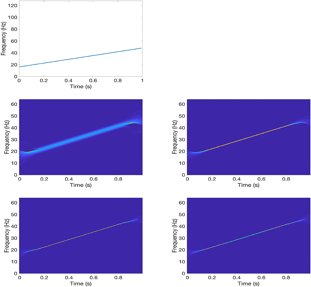
Figure 1. Experiment with x(t) in (43). 1st row: IF ϕ′(t); 2nd row: FSST |R_x(t, η)| (left) and IFE-FSST $\left|R_x^{\text{I}}(t,\eta )\right|$ (right); 3rd row: 2nd-order FSST (left) and 2nd-order IFE-FSST $\left|R_x^{\text{I},2}(t,\eta )\right|$ (right).

For a mono-component signal x(t) as given by (43), since x(t) can be recovered from FSST or IFE-FSST as shown in (8) and (22) respectively, theoretically, either (40) or (41) gives high accurate approximation to x(t) as long as M₀ is large enough. We choose a small M₀ so that the recovery errors with it show how sharp the time-frequency representations with FSST and IFE-FSST are. Here and below we set M₀ = 8.

In Figure 2, we provide the recovery errors $x^{\text{rec}}(t_n)-x(t_n)$, $x^{\text{I},\text{rec}}(t_n)-x(t_n)$ for x(t) by FSST and IFE-FSST, where $x^{\text{rec}}(t_n)$ and $x^{\text{I},\text{rec}}(t_n)$ are given by (40) and (41) respectively with M₀ = 8. Here, we show the error on [0.125, 0.875) only to ignore the boundary effect. Obviously, IFE-FSST provides a much sharper time-frequency representation than FSST.

FIGURE 2

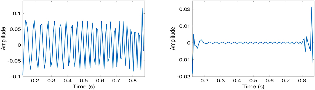
Figure 2. Recovery errors for x(t) given in (43) on [0.125, 0.875) by FSST (left) and IFE-FSST (right).

Next we consider a two-component signal given by

$\begin{array}{l}x\left(t\right)=x_1\left(t\right)+x_2\left(t\right),x_1\left(t\right)=cos\left(2\pi \left(32t+\frac{10}{\pi }cos\left(2\pi t\right)\right)\right),\\ x_2\left(t\right)=cos\left(2\pi \left(64t+\frac{10}{\pi }cos\left(2\pi t\right)\right)\right),& (44)\end{array}$

where t ∈ [0, 2), and x(t) is uniformly sampled with sample points t_n = n△t, 0 ≤ n < N = 512, $△t=\frac{1}{256}$. Thus, IFs of x₁(t), x₂(t) are ${\varphi }_1^{\prime }(t)=32-20sin(2\pi t)$, ${\varphi }_2^{\prime }(t)=64-20sin(2\pi t)$, which are shown on the top-left panel of Figure 3. In this example we let $\sigma =\frac{1}{32}$ for the window function.

FIGURE 3

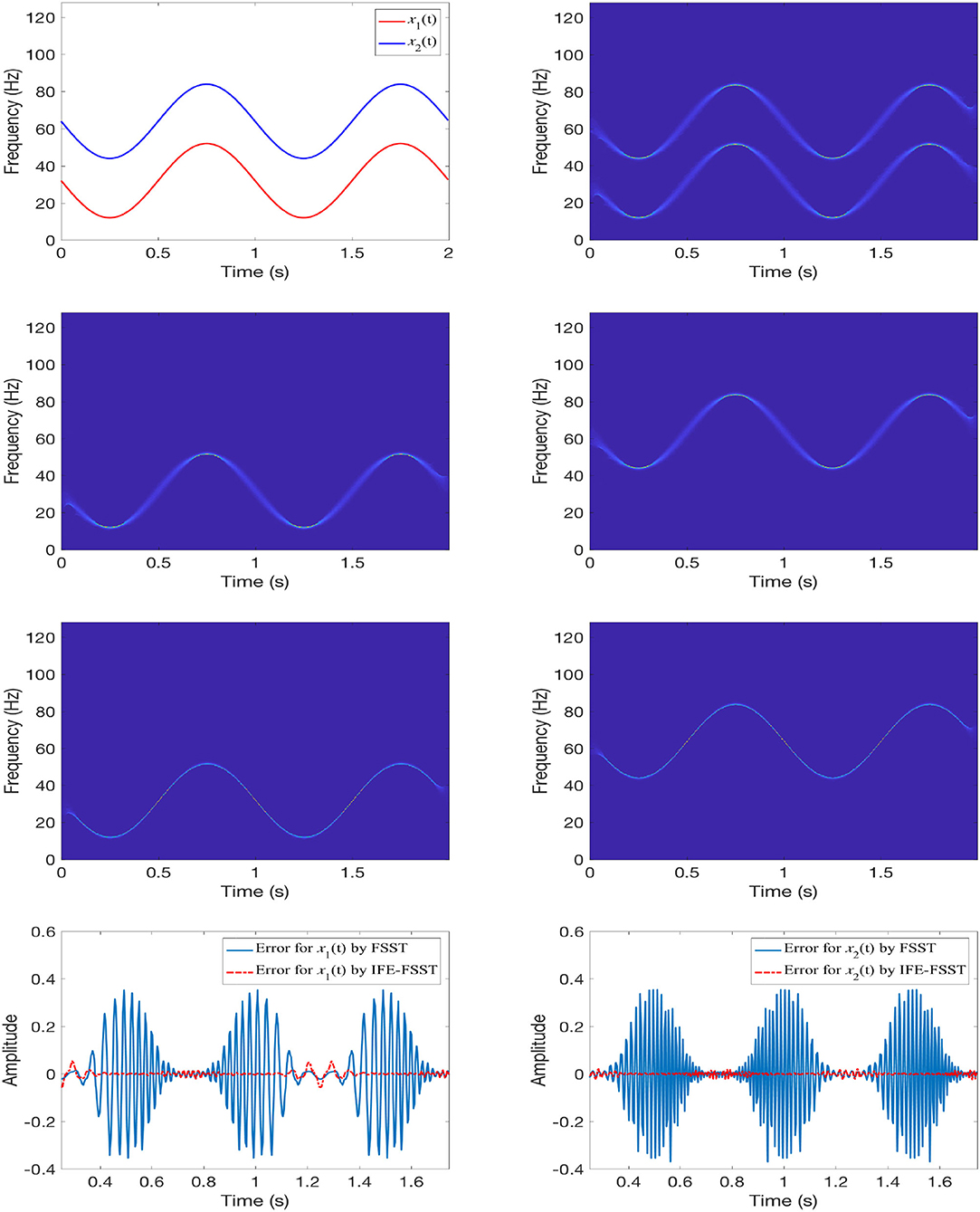
Figure 3. Experiment with x(t) in (44). 1st row: IFs ${\varphi }_1^{\prime }(t),{\varphi }_2^{\prime }(t)$ (left) and FSST |R_x(t, η)| (right); 2nd row: FSST for x₁(t) (left) and FSST for x₂(t) (right); 3rd row: IFE-FSST for x₁(t) (left) and IFE-FSST for x₂(t) (right). 4th row: recovery errors on [0.125, 1.875) by FSST and IFE-FSST for x₁(t) (left) and x₂(t) (right).

To this two-component signal, we apply Algorithm 2 to obtain ${\tilde{x}}_1^{\text{I},\text{rec}}(t)$ and ${\tilde{x}}_2^{\text{I},\text{rec}}(t)$. In the 3rd row of Figure 3 we show the IFE-FSSTs of ${\tilde{x}}_1^{\text{I},\text{rec}}(t)$ and ${\tilde{x}}_2^{\text{I},\text{rec}}(t)$. The FSST of x(t) is provided in the top-right panel of Figure 3. Of course, we can also apply iterative method to FSST to recover components one by one. Namely, we apply FSST to obtain $x_1^{\text{rec}}(t)$, then apply FSST to $x(t)-x_1^{\text{rec}}(t)$ to obtain $x_2^{\text{rec}}(t)$. After that we apply FSST to $x(t)-x_2^{\text{rec}}(t)$ to obtain ${\tilde{x}}_1^{\text{rec}}(t)$, and finally to obtain ${\tilde{x}}_2^{\text{rec}}(t)$ by applying FSST to $x(t)-{\tilde{x}}_1^{\text{rec}}(t)$. The 2nd row of Figure 3 shows the FSSTs of ${\tilde{x}}_1^{\text{rec}}(t)$ and ${\tilde{x}}_2^{\text{rec}}(t)$. Comparing the FSST of x in the top-right panel with the individual FSSTs in the 2nd row, we see there is not much improvement of the time-frequency representation of FSST of x after we apply the iterative component recovery procedure.

In the 4th row of Figure 3, we provide the recovery errors for x₁(t), x₂(t) by FSST and IFE-FSST. Here, we show the error on [0.125, 1.875). From Figure 3, we see IFE-FSST provides a much sharper time-frequency representation for x(t). We also consider FSST and IFE-FSST of two-component x(t) in the noisy environment and our experiments show that IFE-FSST provides a sharp time-frequency representation in the noisy environment. In addition, we consider the 2nd-order IFE-FSST for component recovery. It does not provide much improvement than IFE-FSST. This may be due to that the results from IFE-FSST are hard to improve. Due to that only 15 pictures are allowed to be included in a article in this journal, we do not present these results here.

Data Availability Statement

The original contributions presented in the study are included in the article/supplementary material, further inquiries can be directed to the corresponding author/s.

Ethics Statement

This article was approved by AFRL for public release on 03 Dec. 2021, Case Number: AFRL-2021-4285, Distribution unlimited.

Author Contributions

All authors listed have made a substantial, direct, and intellectual contribution to the work and approved it for publication.

Funding

This work was supported in part by Simons Foundation (Grant No. 353185) and the 2020 Air Force Summer Faculty Fellowship Program (SFFP).

Conflict of Interest

The authors declare that the research was conducted in the absence of any commercial or financial relationships that could be construed as a potential conflict of interest.

Publisher's Note

All claims expressed in this article are solely those of the authors and do not necessarily represent those of their affiliated organizations, or those of the publisher, the editors and the reviewers. Any product that may be evaluated in this article, or claim that may be made by its manufacturer, is not guaranteed or endorsed by the publisher.

References

1. Daubechies I, Lu J, Wu H-T. Synchrosqueezed wavelet transforms: an empirical mode decomposition-like tool. Appl Comput Harmon Anal. (2011) 30:243–61. doi: 10.1016/j.acha.2010.08.002

CrossRef Full Text | Google Scholar

2. Huang NE, Shen Z, Long SR, Wu ML, Shih HH, Zheng Q, et al. The empirical mode decomposition and Hilbert spectrum for nonlinear and nonstationary time series analysis. Proc R Soc Lond A. (1998) 454:903–95. doi: 10.1098/rspa.1998.0193

CrossRef Full Text | Google Scholar

3. Wu Z, Huang NE. Ensemble empirical mode decomposition: a noise-assisted data analysis method. Adv Adapt Data Anal. (2009) 1:1–41. doi: 10.1142/S1793536909000047

PubMed Abstract | CrossRef Full Text | Google Scholar

4. Flandrin P, Rilling G, Goncalves P. Empirical mode decomposition as a filter bank. IEEE Signal Proc Lett. (2004) 11:112–4. doi: 10.1109/LSP.2003.821662

CrossRef Full Text | Google Scholar

5. Li L, Ji H. Signal feature extraction based on improved EMD method. Measurement. (2009) 42:796–803. doi: 10.1016/j.measurement.2009.01.001

CrossRef Full Text | Google Scholar

6. Rilling G, Flandrin P. One or two frequencies? The empirical mode decomposition answers. IEEE Trans Signal Proc. (2008) 56:85–95. doi: 10.1109/TSP.2007.906771

CrossRef Full Text | Google Scholar

7. Lin L, Wang Y, Zhou HM. Iterative filtering as an alternative algorithm for empirical mode decomposition. Adv Adapt Data Anal. (2009) 1:543–60. doi: 10.1142/S179353690900028X

CrossRef Full Text | Google Scholar

8. Xu Y, Liu B, Liu J, Riemenschneider S. Two-dimensional empirical mode decomposition by finite elements. Proc R Soc Lond A. (2006) 462:3081–96. doi: 10.1098/rspa.2006.1700

CrossRef Full Text | Google Scholar

9. van der Walt MD. Empirical mode decomposition with shape-preserving spline interpolation. Results Appl Math. (2020) 5:100086. doi: 10.1016/j.rinam.2019.100086

CrossRef Full Text | Google Scholar

10. Wang Y, Wei G-W, Yang SY. Iterative filtering decomposition based on local spectral evolution kernel. J Sci Comput. (2012) 50:629–64. doi: 10.1007/s10915-011-9496-0

PubMed Abstract | CrossRef Full Text | Google Scholar

11. Zheng JD, Pan HY, Liu T, Liu QY. Extreme-point weighted mode decomposition. Signal Proc. (2018) 42:366–74. doi: 10.1016/j.sigpro.2017.08.00

PubMed Abstract | CrossRef Full Text | Google Scholar

12. Cicone A, Liu JF, Zhou HM. Adaptive local iterative filtering for signal decomposition and instantaneous frequency analysis. Appl Comput Harmon Anal. (2016) 41:384–411. doi: 10.1016/j.acha.2016.03.001

PubMed Abstract | CrossRef Full Text | Google Scholar

13. Thakur G, Wu H-T. Synchrosqueezing based recovery of instantaneous frequency from nonuniform samples. SIAM J Math Anal. (2011) 43:2078–95. doi: 10.1137/100798818

CrossRef Full Text | Google Scholar

14. Wu H-T. Adaptive analysis of complex data sets. Ph.D. dissertation. Princeton University Press, Princeton, NJ, United States (2012).

15. Oberlin T, Meignen S, Perrier V. The Fourier-based synchrosqueezing transform. In: Proc. 39th Int. Conf. Acoust., Speech, Signal Proc. (ICASSP). Beijing (2014). p. 315–9. doi: 10.1109/ICASSP.2014.6853609

CrossRef Full Text | Google Scholar

16. Oberlin T, Meignen S, Perrier V. Second-order synchrosqueezing transform or invertible reassignment? Towards ideal time-frequency representations. IEEE Trans Signal Proc. (2015) 63:1335–44. doi: 10.1109/TSP.2015.2391077

PubMed Abstract | CrossRef Full Text | Google Scholar

17. Oberlin T, Meignen S. The 2nd-order wavelet synchrosqueezing transform. In: 2017 IEEE International Conference on Acoustics, Speech and Signal Processing (ICASSP). New Orleans, LA (2017). doi: 10.1109/ICASSP.2017.7952906

CrossRef Full Text | Google Scholar

18. Lu J, Alzahrani JH, Jiang QT. A second-order synchrosqueezing transform with a simple phase transformation. Num Math Theory Methods Appl. (2021) 14: 624–49. doi: 10.4208/nmtma.OA-2020-0077

CrossRef Full Text | Google Scholar

19. Pham D-H, Meignen S. High-order synchrosqueezing transform for multicomponent signals analysis - With an application to gravitational-wave signal. IEEE Trans Signal Proc. (2017) 65:3168–78. doi: 10.1109/TSP.2017.2686355

CrossRef Full Text | Google Scholar

20. Li L, Wang ZH, Cai HY, Jiang QT, Ji HB. Time-varying parameter-based synchrosqueezing wavelet transform with the approximation of cubic phase functions. In: 2018 14th IEEE Int'l Conference on Signal Proc. ICSP. New Orleans, LA (2018). p. 844–8. doi: 10.1109/ICSP.2018.8652362

CrossRef Full Text | Google Scholar

21. Chui CK, van der Walt MD. Signal analysis via instantaneous frequency estimation of signal components. Int J Geomath. (2015) 6:1–42. doi: 10.1007/s13137-015-0070-z

CrossRef Full Text | Google Scholar

22. Chui CK, Lin Y-T, Wu H-T. Real-time dynamics acquisition from irregular samples - with application to anesthesia evaluation. Anal Appl. (2016) 14:537–90. doi: 10.1142/S0219530515500165

CrossRef Full Text | Google Scholar

23. Daubechies I, Wang Y, Wu H-T. ConceFT: concentration of frequency and time via a multitapered synchrosqueezed transform. Philos Trans R Soc A. (2016) 374:20150193. doi: 10.1098/rsta.2015.0193

PubMed Abstract | CrossRef Full Text | Google Scholar

24. Yang HZ. Synchrosqueezed wave packet transforms and diffeomorphism based spectral analysis for 1D general mode decompositions. Appl Comput Harmon Anal. (2015) 39:33–66. doi: 10.1016/j.acha.2014.08.004

CrossRef Full Text | Google Scholar

25. Yang HZ, Ying LX. Synchrosqueezed curvelet transform for two-dimensional mode decomposition. SIAM J. Math Anal. (2014) 3:2052–83. doi: 10.1137/130939912

CrossRef Full Text | Google Scholar

26. Sheu Y-L, Hsu L-Y, Chou P-T, Wu H-T. Entropy-based time-varying window width selection for nonlinear-type time-frequency analysis. Int J Data Sci Anal. (2017) 3:231–45. doi: 10.1007/s41060-017-0053-2

CrossRef Full Text | Google Scholar

27. Berrian AJ, Saito N. Adaptive synchrosqueezing based on a quilted short-time Fourier transform. arXiv [Preprint] arXiv:1707.03138v5. (2017). doi: 10.1117/12.2271186

PubMed Abstract | CrossRef Full Text | Google Scholar

28. Li L, Cai HY, Han HX, Jiang QT, Ji HB. Adaptive short-time Fourier transform and synchrosqueezing transform for non-stationary signal separation. Signal Proc. (2020) 166:107231. doi: 10.1016/j.sigpro.2019.07.024

CrossRef Full Text | Google Scholar

29. Li L, Cai HY, Jiang QT. Adaptive synchrosqueezing transform with a time-varying parameter for non-stationary signal separation. Appl Comput Harmon Anal. (2020) 49:1075–106. doi: 10.1016/j.acha.2019.06.002

CrossRef Full Text | Google Scholar

30. Cai HY, Jiang QT, Li L, Suter BW. Analysis of adaptive short-time Fourier transform-based synchrosqueezing transform. Anal Appl. (2021) 19:71–105. doi: 10.1142/S0219530520400047

CrossRef Full Text | Google Scholar

31. Lu J, Jiang QT, Li L. Analysis of adaptive synchrosqueezing transform with a time-varying parameter. Adv Comput Math. (2020) 46:72. doi: 10.1007/s10444-020-09814-x

CrossRef Full Text | Google Scholar

32. Li C, Liang M. Time frequency signal analysis for gearbox fault diagnosis using a generalized synchrosqueezing transform. Mech Syst Signal Proc. (2012) 26:205–17. doi: 10.1016/j.ymssp.2011.07.001

PubMed Abstract | CrossRef Full Text | Google Scholar

33. Wang SB, Chen XF, Selesnick IW, Guo YJ, Tong CW, Zhang XW. Matching synchrosqueezing transform: a useful tool for characterizing signals with fast varying instantaneous frequency and application to machine fault diagnosis. Mech Syst Signal Proc. (2018) 100:242–88. doi: 10.1016/j.ymssp.2017.07.009

CrossRef Full Text | Google Scholar

34. Wu H-T. Current state of nonlinear-type time-frequency analysis and applications to high-frequency biomedical signals. Curr Opin Syst Biol. (2020) 23:8–21. doi: 10.1016/j.coisb.2020.07.013

CrossRef Full Text | Google Scholar

35. Chui CK, Mhaskar HN. Signal decomposition and analysis via extraction of frequencies. Appl Comput Harmon Anal. (2016) 40:97–136. doi: 10.1016/j.acha.2015.01.003

CrossRef Full Text | Google Scholar

36. Li L, Chui CK, Jiang QT. Direct signal separation via extraction of local frequencies with adaptive time-varying parameter. arXiv [Preprint] arXiv:2010.01866. (2020).

Google Scholar

37. Chui CK, Jiang QT, Li L, Lu J. Analysis of an adaptive short-time Fourier transform-based multicomponent signal separation method derived from linear chirp local approximation. J Comput Appl Math. (2021) 396:113607. doi: 10.1016/j.cam.2021.113607

CrossRef Full Text | Google Scholar

38. Chui CK, Han NN. Wavelet thresholding for recovery of active sub-signals of a composite signal from its discrete samples. Appl Comput Harmon Anal. (2021) 52:1–24. doi: 10.1016/j.acha.2020.11.003

CrossRef Full Text | Google Scholar

39. Chui CK, Jiang QT, Li L, Lu J. Signal separation based on adaptive continuous wavelet-like transform and analysis. Appl Comput Harmon Anal. (2021) 53:151–79. doi: 10.1016/j.acha.2020.12.003

CrossRef Full Text | Google Scholar

40. Chui CK, Mhaskar HN, van der Walt MD. Data-driven atomic decomposition via frequency extraction of intrinsic mode functions. Int J Geomath. (2016) 7:117–46. doi: 10.1007/s13137-015-0079-3

CrossRef Full Text | Google Scholar

41. Li C, Liang M. A generalized synchrosqueezing transform for enhancing signal time-frequency representation. Signal Proc. (2012) 92:2264–74. doi: 10.1016/j.sigpro.2012.02.019

CrossRef Full Text | Google Scholar

42. Meignen S, Pham D-H, McLaughlin S. On demodulation, ridge detection, and synchrosqueezing for multicomponent signals. IEEE Trans Signal Proc. (2017) 65:2093–103. doi: 10.1109/TSP.2017.2656838

CrossRef Full Text | Google Scholar

43. Wang SB, Chen XF, Cai GG, Chen BQ, Li X, He ZJ. Matching demodulation transform and synchrosqueezing in time-frequency analysis. IEEE Trans Signal Proc. (2014) 62:69–84. doi: 10.1109/TSP.2013.2276393

CrossRef Full Text | Google Scholar

44. Jiang QT, Suter BW. Instantaneous frequency estimation based on synchrosqueezing wavelet transform. Signal Proc. (2017) 138:167–81. doi: 10.1016/j.sigpro.2017.03.007

PubMed Abstract | CrossRef Full Text | Google Scholar

45. Stankovic L, Dakovic M, Ivanovic V. Performance of spectrogram as IF estimator. Electron Lett. (2001) 37:797–9. doi: 10.1049/el:20010517

PubMed Abstract | CrossRef Full Text | Google Scholar