A Knowledge-Aided Robust Ensemble Kalman Filter Algorithm for Non-Linear and Non-Gaussian Large Systems

This work proposes a robust and non-Gaussian version of the shrinkage-based knowledge-aided EnKF implementation called Ensemble Time Local H_∞ Filter Knowledge-Aided (EnTLHF-KA). The EnTLHF-KA requires a target covariance matrix to integrate previously obtained information and knowledge directly into the data assimilation (DA). The proposed method is based on the robust H_∞ filter and on its ensemble time-local version the EnTLHF, using an adaptive inflation factor depending on the shrinkage covariance estimated matrix. This implies a theoretical and solid background to construct robust filters from the well-known covariance inflation technique. The proposed technique is implemented in a synthetic assimilation experiment, and in an air quality application using the LOTOS-EUROS model over the Aburrá Valley to evaluate its potential for non-linear and non-Gaussian large systems. In the spatial distribution of the PM_2.5 concentrations along the valley, the method outperforms the well-known Local Ensemble Transform Kalman Filter (LETKF), and the non-robust knowledge-aided Ensemble Kalman filter (EnKF-KA). In contrast to the other simulations, the ability to issue warnings for high concentration events is also increased. Finally, the simulation using EnTLHF-KA has lower error values than using EnKF-KA, indicating the advantages of robust approaches in high uncertainty systems.

1. Introduction

Data assimilation (DA) is a mathematical family of methods that allows the combination of observations and models. The model is used to fill observational gaps, and the observations constrain the model dynamics [1, 2]. In most DA methods, the aim is to minimize the estimated error variance. For instance, Kalman filter (KF) is an optimal method that minimizes the mean-squared-error in the estimation. The KF is optimal when the dynamic system is linear [3]. The Ensemble Kalman filter (EnKF) is a KF-based Monte Carlo approximation of the KF when the state space is large, and the model is non-linear [4]. The EnKF uses an ensemble of model realizations to approximate the first and second background error moments, making it efficient for large-scale models and suitable in the presence of non-linearities. However, in real DA applications, the assumptions required to obtain the optimal solution may not be accurate, degrading the filter performance [4, 5]. Additionally, small ensemble sizes may produce a poor approximation of the model uncertainty, causing a reduction in the filter accuracy or even filter divergence. When the system conditions do not satisfy the requirements of the KF-based method, the robust filters are a powerful and practical alternative to solve the estimation problem. Motivated by robust control ideas that have been established over many years in the field of control engineering [6], the robust filters emphasize the robustness of the estimation to have better tolerances to high uncertainty sources. Since their purpose is not the optimality in the estimation, the robust estimators do not require a strictly statistical representation of the system and the observations [7], showing a better performance than the KF-based methods in scenarios with a poor statistical uncertainty representation [8, 9]. There are several robust ensemble-based DA schemes based on different principles such as H_∞ formulation [8], replacing the traditional L₂ norm [10–12], robust covariance estimation [13, 14], and covariance inflation [6, 7]. The approach that we propose uses a shrinkage-based covariance estimator that improves the model robustness and performance when the ensemble size is small [15]. Additionally, our method incorporates adaptive covariance inflation closely related to the H_∞ formulation.

The uncertainty in chemical transport models (CTM) simulations could be reduced by the improvement of the emission inventory and the upgrade of meteorological data. Alternatively one could incorporate ground data, satellite information, or vertical in the simulations using DA techniques to reduce the uncertainty [16–19]. In Lopez et al.'s [19] study, DA over the Aburrá Valley has been applied using the LOTOS-EUROS CTM, building on earlier applications [16–18]. Aburrá Valley's pollution-related air quality issues have become worse over the last 10 years. Due to the Valley's meteorological dynamics transitioning between dry and rainy seasons, the air quality deteriorates two times a year dramatically, around the arrival of the Intertropical Convergence Zone (March-April, and with lower intensity in October-November) [20, 21]. During these times, the atmospheric boundary layer remains below the canyon's rim throughout the day, trapping all of the pollutants from the city in the lower atmosphere. The resulting concentrations of particulate matter smaller than 10 μm (PM₁₀) and 2.5 μm (PM_2.5) remain at levels considered hazardous for the general population, leading to bi-annual periods of worsened air quality known locally as “environmental contingencies,” during which special measures are taken. In this study, the application of the LOTOS-EUROS CTM to reproduce the PM_2.5 over the valley integrating ground based observations is taken as a real-life study case.

The study is organized as follows. section 2 describes the basic concepts of DA used and introduces the derivation of the proposed method. In section 3 using numerical experiments with a low-scale model, we compare the proposed method's robustness and performance against its related DA algorithms. In section 4, we show the evaluation of the proposed method in a real-life and complex application and discuss the results in terms of investigating the ability to reproduce particulate matter concentrations and forecasting capability of the proposed method. Finally, section 5 offers some concluding remarks and outlines the needed future work. The CTM implementation description is presented in the Appendix.

2. Robust Ensemble-based DA Using Prior Knowledge

In ensemble-based DA, an ensemble of model realizations

$\begin{array}{ll}{\text{X}}^b=\left[{\text{x}}^{b\left[1\right]},{\text{x}}^{b\left[2\right]},\dots ,{\text{x}}^{b\left[N\right]}\right]\in {ℝ}^{n\times N},& (1)\end{array}$

is employed to estimate the first (x^b) and second moments (B) of the background error distributions, where x^b[i] ∈ ℝ^n×1 is the i-th ensemble member, and N is the total number of ensemble members. Hence

$\begin{array}{ll}{\text{x}}^b\approx {\overline{\text{x}}}^b=\frac{1}{N-1}·{\displaystyle \sum _{e=1}^N}{\text{x}}^{b\left[e\right]}\in {ℝ}^{n\times 1},& (2)\end{array}$

and

$\begin{array}{ll}\text{B}\approx {\text{P}}^b=\frac{1}{N}·\Delta \text{X}·{\Delta \text{X}}^T\in {ℝ}^{n\times n},& (3)\end{array}$

where

$\begin{array}{ll}\Delta \text{X}={\text{X}}^b-{\overline{\text{x}}}^b·1^T\in {ℝ}^{n\times N},& (4)\end{array}$

is the anomalies matrix, ${\overline{\text{x}}}^b$ is the ensemble mean, P^b is the sample covariance matrix, and 1 is a vector with components all ones. Once an observation is available, the posterior state can be computed via an ensemble-based method as EnKF [4] or its variants, EnKS [4], EnHF [22], or 4DEnVAR [22] for instance. The widely-used stochastic EnKF computed the analysis state as a combination of the prior state and the differences between the observations and model outputs is the following [4]:

$\begin{array}{ll}{\text{X}}^a={\text{X}}^b+{\text{P}}^b·{\text{H}}^T·{\left[\text{R}+\text{H}·{\text{P}}^b·{\text{H}}^T\right]}^{-1}·\text{D}\in {ℝ}^{n\times N},& (5)\end{array}$

where X^a is the analysis ensemble, H is the linear (or linearized) output operator, and the e-th column of the innovation matrix on the synthetic observations D ∈ ℝ^n×N reads ${\text{d}}^{\left[e\right]}=\text{y}+{ϵ}^{\left[e\right]}-{H}\left({\text{x}}^{b\left[e\right]}\right)\in {ℝ}^{m\times 1}$, with ${ϵ}^{\left[e\right]}~{N}(0,\text{R})$. The quality of analysis corrections is directly impacted by the accuracy in the estimation of B throw P^b, which is highly susceptible to the limited number of ensemble members, the state distribution, and the system uncertainty quantification.

2.1. LETKF

One of the most commonly used implementations of the EnKF method is the local ensemble transform Kalman filter (LETKF) [23], where the assimilation process is performed independently for each model variable. Around each model variable (grid point), a sub-domain of radius r is constructed, and the assimilation process is carried out within the local domain. Each local analysis is mapped onto the global domain to obtain the global analysis, and the assimilation is completed. In the assimilation process, all the information found within the sub-domain (i.e., observed components and error correlations) is used. LETKF's local approach has made it an interesting alternative for application in large-scale systems, so we use this method as a baseline to compare our proposed algorithm. The analysis state could be obtained following the implementation by Shin et al. [24] :

$\begin{array}{ll}\Delta \text{X}={\text{X}}^b-{\overline{\text{x}}}^b·1^T\in {ℝ}^{n\times N},& (\mathrm{6a})\end{array}$

$\begin{array}{ll}\Delta \text{Y}=\text{H}·\Delta \text{X}& (\mathrm{6b})\end{array}$

$\begin{array}{ll}{\text{P}}^a={\left[\Delta {\text{Y}}^T·{\text{R}}^{-1}·\Delta \text{Y}+(m-1)·\text{I}\right]}^{-1},& (\mathrm{6c})\end{array}$

$\begin{array}{ll}\text{D}=\text{y}-\text{H}·{\overline{\text{x}}}^b,& (\mathrm{6d})\end{array}$

$\begin{array}{ll}{\text{w}}^a={\text{P}}^a·{\text{Y}}^T·{\text{R}}^{-1}·\text{D},& (6e)\end{array}$

$\begin{array}{ll}{\overline{\text{x}}}^a={\overline{\text{x}}}^b+\Delta \text{X}·{\text{w}}^a,& (\mathrm{6f})\end{array}$

$\begin{array}{ll}{\text{X}}^a={\text{X}}^b·{\left[(n-1)·{\text{P}}^a\right]}^{1/2},& (\mathrm{6g})\end{array}$

where n, m, and N are the model resolution, the number of observations, and the number of ensemble members, respectively, P^a ∈ ℝ^n×n is the analysis ensemble covariance matrix, and 1 is a vector of the consistent dimension whose components are all ones. In the LETKF algorithm, the above analysis is applied per grid cell. The algorithm uses the following steps:

1. Compute in each domain simulated observations for all ensemble members.

2. Collect per domain also the observations from neighboring domains that are within r distance

3. Loop over grid cells.

(a) Select observations and simulations that are within range r.

(b) Compute analysis weights w^a.

(c) Apply the analysis with the ensemble elements for the selected grid cell.

4. Once all the local analyses are performed, map those to the global domain.

Note that the background error covariance matrix approximation in the LETKF is the sample covariance matrix (3), therefore for large radii of influence, the quality of the LETKF results could be influenced by spurious correlations.

2.2. Shrinkage-Based ENKF

A more robust family of covariance estimators for the case n ≫ N are the shrinkage based estimators [25, 26]. These kinds of estimators have the form [27]:

$\begin{array}{ll}\text{B}\approx \hat{\text{B}}(\alpha )=\alpha ·\text{T}+(1-\alpha )·{\text{P}}^b\in {ℝ}^{n\times n},& (7)\end{array}$

where α ∈ [0, 1], and T ∈ ℝ^n×n is a user-defined matrix. The value of α is chosen to minimize

$\begin{array}{ll}{\alpha }^{*}=arg{\displaystyle \underset{\alpha }{min}}𝔼\left[\Vert \text{B}-\hat{\text{B}}(\alpha ){\Vert }_F^2\right],& (8)\end{array}$

where ||•||_F represents the Frobenius norm. A close formulation to calculate the weight value α using a general target matrix T_KA is proposed in [28, 29] (hereafter KA estimator),

$\begin{array}{ll}{\widehat{\text{B}}}_{KA}={\alpha }_{KA}·{\text{T}}_{KA}+(1-{\alpha }_{KA})·{\text{P}}^b\in {ℝ}^{n\times n},& (\mathrm{9a})\end{array}$

with

$\begin{array}{ll}{\alpha }_{KA}=min\left(\frac{\frac{1}{N^2}·{\displaystyle {\sum }_{i=1}^N}\Vert {\Delta \text{x}}^{\left[e\right]}{\Vert }^4-\frac{1}{N}·\Vert {\text{P}}^{\text{b}}{\Vert }^2}{\Vert {\text{P}}^b-{\text{T}}_{KA}{\Vert }^2},1\right).& (\mathrm{9b})\end{array}$

This general target matrix enables the incorporation of prior information about the system into the error covariance matrix. Although T_KA must meet all requirements of a covariance matrix, T_KA must not fulfill any requirement about its structure and also can change dynamically, allowing a complete degree of freedom in the matrix computation. Sections 3, 4, and Lopez-Restrepo et al. [15] show some examples of how to compute T_KA. Additionally, the KA estimator does not make any distributional assumptions, thus can also be used for non-Gaussian covariance matrix estimation [29]. An implementation of the EnKF can be obtained using the KA estimator, known as EnKF-KA [15]:

$\begin{array}{l}{\text{X}}^a={\text{X}}^b+{\widehat{\text{B}}}_{KA}·{\text{H}}^T·\left[\text{R}+\text{H}·{\widehat{\text{B}}}_{KA}·{\text{H}}^T\right]·\text{D}.\end{array}$

In Lopez-Restrepo et al. [19], it is shown that incorporating prior information of the system in the data assimilation process can outperform the EnKF when n ≫ N, and when, there are errors in the model specifications.

2.3. Ensemble Time-Local H_∞ Filter

One of the most widely used robust filter is the H_∞ Filter (HF) [30]. The HF is based on the criterion of minimizing the supremum of the L₂ norm of the uncertainty sources [8]. The ideas beyond the HF filters come from the robust control theory and applications in linear and low-scale systems [31]. In recent years, several works have been started to develop implementations of the HF in DA due to its potential to solve some limitations of the EnKF [6, 7, 9, 31]. The HF ensures that the total energy of the estimation errors, is not larger than the uncertainty energy times a factor 1/γ:

$\begin{array}{l}{\displaystyle \sum _{k=0}^M}\Vert {\text{x}}_k^t-{\text{x}}_k^a{\Vert }_{{\text{S}}_k}^2\le \frac{1}{\gamma }(\Vert {\text{x}}_0^t-{\text{x}}_0^a{\Vert }_{{\Delta }_0^{-1}}^2+{\displaystyle \sum _{k=0}^M}\Vert {\text{u}}_k{\Vert }_{{\text{Q}}_k^{-1}}^2\\ +{\displaystyle \sum _{k=0}^M}\Vert {\text{v}}_k{\Vert }_{{\text{R}}_k^{-1}}^2),& (10)\end{array}$

where x^t is the true state, x^a is the analysis state, S is a user-chosen matrix of weights, u and v are the model and observation uncertainty, respectively, Δ₀, Q, and R are the uncertainty weighting matrices with respect to the initial conditions, model error, and observations error, and M is the DA windows length [7]. To solve (10), the cost function ${{J}}^{HF}$ is defined as follows:

$\begin{array}{ll}{{J}}^{HF}=\frac{{\displaystyle {\sum }_{k=0}^M}\Vert {\text{x}}_k^t-{\text{x}}_k^a{\Vert }_{{\text{S}}_k}^2}{\Vert {\text{x}}_0^t-{\text{x}}_0{\Vert }_{{\Delta }_0^{-1}}^2+{\displaystyle {\sum }_{k=0}^M}\Vert {\text{u}}_k{\Vert }_{{\text{Q}}_k^{-1}}^2+{\displaystyle {\sum }_{k=0}^M}\Vert {\text{v}}_k{\Vert }_{{\text{R}}_k^{-1}}^2}.& (11)\end{array}$

Then inequality (10) is equivalent to ${{J}}^{HF}\le \frac{1}{\gamma }$. Let γ^* be the value such that

$\begin{array}{ll}\frac{1}{{\gamma }^{*}}={\displaystyle \underset{\{{\text{x}}_k^a\}}{inf}}{\displaystyle \underset{{\text{x}}_0,\{{\text{u}}_k\},\{{\text{v}}_k\}}{sup}}{{J}}^{HF},k\le M,& (12)\end{array}$

the optimal HF is then achieved when γ = γ^*. In this formulation, the evaluation of γ^* is an application of the minimax rule [32], a strategy that aims to provide robust estimates and is different from its Bayesian counterpart [7]. An Ensemble-based HF implementation for a nonlinear DA problem is the Ensemble time-local H_∞ filter (EnLTHF) proposed by Luo et al. [7]. In the EnLTHF, a local cost function is proposed:

$\begin{array}{ll}{{J}}_k^{HF}=\frac{\Vert {\text{x}}_k^t-{\text{x}}_k^a{\Vert }_{{\text{S}}_k}^2}{\Vert {\text{x}}_0^t-{\text{x}}_0{\Vert }_{{\Delta }_0^{-1}}^2+\Vert {\text{u}}_k{\Vert }_{{\text{Q}}_k^{-1}}^2+\Vert {\text{v}}_k{\Vert }_{{\text{R}}_k^{-1}}^2}.& (13)\end{array}$

The local performance level γ_k satisfies:

$\begin{array}{ll}\frac{1}{{\gamma }_k}\ge \frac{1}{{\gamma }_k^{*}}={\displaystyle \underset{\{{\text{x}}_k^a\}}{inf}}{\displaystyle \underset{{\text{x}}_0,\{{\text{u}}_k\},\{{\text{v}}_k\}}{sup}}{{J}}_k^{HF},& (14)\end{array}$

The EnLTHF can be expressed in terms of the EnKF algorithm using the notation of Luo et al. [7]:

$\begin{array}{ll}\left[{\text{P}}_k^a,{\text{K}}_k\right]=EnKF({\text{x}}_k^a,{\text{Q}}_k,\text{H}),& (\mathrm{15a})\end{array}$

$\begin{array}{ll}{\text{G}}_k={\left[I_m-{\gamma }_k·{\text{P}}_k^a·{\text{S}}_k\right]}^{-1}·{\text{K}}_k,& (\mathrm{15b})\end{array}$

$\begin{array}{ll}{\text{x}}_k^{a(i)}={\text{x}}_k^{b(i)}+{\text{G}}_{\text{k}}·\left[{\text{y}}_{\text{k}}-{\text{H}}_{\text{k}}·{\text{x}}_{\text{k}}^{\text{b}(\text{i})}+{\text{v}}_{\text{k}}^{\text{i}}\right],& (\mathrm{15c})\end{array}$

$\begin{array}{ll}{\text{x}}_k^a=\left({\displaystyle \sum _{i=1}^N}{\text{x}}_k^{a(i)}\right)/N,& (\mathrm{15d})\end{array}$

$\begin{array}{ll}{({\Delta }_{\text{k}}^{\text{a}})}^{-1}={({\text{P}}_k^a)}^{-1}-{\gamma }_k·{\text{S}}_k,& (15e)\end{array}$

subject to the constraint

$\begin{array}{ll}{({\Delta }_k^a)}^{-1}={({\text{P}}_k^a)}^{-1}-{\gamma }_k·{\text{S}}_k\ge 0,& (\mathrm{15f})\end{array}$

where the operator EnKF(·, ·, ·) means that ${\text{P}}_k^a$ and K_k are obtained through the EnKF.

2.4. Adaptive Inflation

A particular issue with ensemble-based DA algorithms is the covariance undersampling. Undersampling leads to further problems such as the ensemble collapse to an overconfident, but incorrect state, or even filter divergence [33]. The covariance inflation artificially increases uncertainties in the background covariance avoiding the underestimation of uncertainties and undersampling [34]. The magnitude of the inflation depends to a large degree on each system and application [35].

In (15e), the presence of the extra term −γ_k · S_k inflates the EnKF covariance matrix. In this way, it is possible to interpret the EnTLHF as an EnKF formulation with a specific value of inflation. This implies a theoretical and solid background to construct robust filters. Consider the case where S = I_n, which corresponds with an inflation of the analysis covariance matrix eigenvalues. To satisfy the constraint (15f), or what is equivalent, to make ${({\Delta }_k^a)}^{-1}$ semi-definite positive, consider the SVD decomposition of ${\text{P}}_k^a$

$\begin{array}{ll}{\text{P}}_k^a={\text{V}}_{\text{k}}·{\Sigma }_{\text{k}}·{\text{U}}_{\text{k}},& (16)\end{array}$

where Σ_k = diag(σ_t,1, ..., σ_t,n) is a diagonal matrix with all the eigenvalues of ${\text{P}}_k^a$ in descending order, that is, σ_t,1 ≥ σ_t,2 ≥ .... ≥ σ_t,n and γ_k is a variable that satisfies

$\begin{array}{l}{{\sigma }_{t,1}}^{-1}-{\gamma }_k\ge 0,\end{array}$

that corresponds with

$\begin{array}{l}{\gamma }_k\le \frac{1}{{\sigma }_{t,1}},\end{array}$

guaranteeing that ${({\Delta }_{\text{k}}^{\text{a}})}^{-1}$ is semi-definite positive. It is convenient to introduce a performance level coefficient (PLC) c by defining

$\begin{array}{ll}{\gamma }_k\le \frac{c}{{\sigma }_{t,1}}.& (17)\end{array}$

In contrast to conventional inflation schemes, γ_k is adaptive in time even for a fixed c value, and it is directly related with the analysis covariance matrix.

2.5. Ensemble Time Local H_∞ Filter Knowledge Aided (EnTLHF-KA)

According to sections 2.3 and 2.4, with a specific structure and inflation value, it is possible to obtain a robust version of the EnKF. Although the EnTLHF has shown to have a better performance than the EnKF in scenarios with high uncertainty [7, 36, 37], the limitations of the EnKF with respect to the ensemble size and the ensemble normality distribution are inherited in its robust version. When the ensemble size is small N << n, sampling errors can have an impact on the quality of covariances matrix estimation, causing problems such as filter divergence and spurious correlations [4, 35]. Even though many localization techniques have been developed to mitigate those problems, it usually prohibits its implementation in high dimensional applications [38]. The shrinkage-covariance estimator methods have shown a better performance than the classical sampling covariance matrix in scenarios with small ensemble sizes and non-Gaussianities [27, 39–41].

We propose a robust implementation of the EnKF-KA shrinkage-based method following the principles of the EnTLHF and the adaptive inflation denoted EnTLHF-KA. The EnTLHF-KA can be obtained similarly to the EnLTHF by taking as base the EnKF-KA:

$\begin{array}{ll}\left[{\widehat{\text{B}}}_{KA}^a,{\text{K}}_k\right]=\text{EnKF-KA}({\text{x}}_k^a,{\text{T}}_{KA},\text{H}),& (\mathrm{18a})\end{array}$

$\begin{array}{ll}{\text{G}}_{\text{k}}={\left[I_m-{\gamma }_k·{\widehat{\text{B}}}_{KA}^a·{\text{S}}_k\right]}^{-1}·{\text{K}}_k,& (\mathrm{18b})\end{array}$

$\begin{array}{ll}{\text{x}}_k^{a(i)}={\text{x}}_k^{b(i)}+{\text{G}}_{\text{k}}·[{\text{y}}_{\text{k}}-{\text{H}}_{\text{k}}·{\text{x}}_{\text{k}}^{\text{b}(\text{i})}+{\text{v}}_{\text{k}}^{\text{i}}],& (\mathrm{18c})\end{array}$

$\begin{array}{ll}{\text{x}}_k^a=\left({\displaystyle \sum _{i=1}^N}{\text{x}}_k^{a(i)}\right)/N,& (\mathrm{18d})\end{array}$

where the operator EnKF-KA(·, ·, ·) represents the EnKF-KA shrinkage-based method (see section 2.2). For a specific PLC, the inflation value is obtained using (17).

3. Results in Low-Scale System

A series of synthetic DA experiments allow us to expose the robust filter benefits over the former methods and evaluate the robustness with controlled scenarios. The Lorenz-96 is one of the most used benchmarks for testing DA algorithms. The model is highly non-linear and with a strong relationship between the states. The Lorenz-96 dynamics are described by [42, 43]:

$\begin{array}{ll}\frac{d{x}_j}{dt}=\{\begin{array}{ll}(x_2-x_{n-1})·x_n-x_1+F& \text{for }j=1,\\ (x_{j+1}-x_{j-2})·x_{j-1}-x_j+F& \text{for }2\le j\le n-1,\\ (x_1-x_{n-2})·x_{n-1}-x_n+F& \text{for }j=n,\end{array}& (19)\end{array}$

where n is the state number chosen as 40 and F is the external force. For consistency, periodic boundary conditions are assumed. We take the next considerations for the numerical experiments:

• The assimilation window consists of M = 500 observations.

• The number of observed components is m = 20, representing 50% of the model components.

• The observation statistics are associated with the Gaussian distribution,

$\begin{array}{ll}{\text{y}}_t~{N}(\text{H}·{\text{x}}_t^a,{\rho }_o^2·\text{I}),\text{for }1\le t\le M,& (20)\end{array}$

where ρ_o = 0.001, and H is a linear operator that randomly chooses the m observed components.

• To avoid random fluctuations, each experiment is repeated 20 times (L = 20).

• We compare the performance and robustness of the EnTLHF-KA against the non-robust methods EnKF and EnKF-KA, and the robust method EnTLHF.

• We use a Gaspari-Cohn [44] matrix with an influence radius of 2 as target matrix T_KA for the EnKF-KA and the EnTLHF-KA. Following [7], we do not use covariance localization to avoid complicating the analysis of our experiment results.

• We take the Root-Mean-Square-Error (RMSE) of L experiments as a measure of performance,

$\begin{array}{ll}\text{RMSE}=\frac{1}{L}·{\displaystyle \sum _{l=1}^L}\left(\sqrt{\frac{1}{M}·{\displaystyle \sum _{t=1}^M}{\left({\left[{\text{x}}_t^{*}-{\text{x}}_t^a\right]}^T·\left[{\text{x}}_t^{*}-{\text{x}}_t^a\right]\right)}^2}\right).& (21)\end{array}$

• We chose a PLC value c = 0.5 for all the experiments, following Luo and Hoteit [7]. Other c values have been tested (not reported here), but no performance improvements were obtained.

3.1. Robustness Against Ensemble Members

When the state dimension is large, it is important to test the performance with relative small ensemble sizes. We evaluate both the accuracy and the robustness of the EnTLHF-KA with respect to the ensemble size. For this case, we set the observation error δ= 1 × 10⁻³, the observation frequency f = 1, and the external force F = 8. The ensemble size N ∈ [10, 20, 50, 100, 1, 000]. Figure 1 presents the RMSE value for those values of N.

FIGURE 1

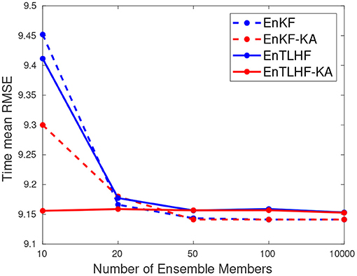
Figure 1. Error evaluation of the robust and non-robust methods with respect to the ensemble member number.

The EnTLHF-KA has more constant RMSE values for different N. The other methods present variation in its performance when the ensemble size changes. In general, the RMSE values decrease for larger N values for all the methods. For N = 10, the EnTLHF-KA presents a superior performance compared to the others, followed by the EnKF-KA. This behavior is attributed to the shrinkage-based estimator used in both methods, that have shown a better covariance estimation when N << n [19, 41]. However, the adaptive inflation factor of the EnTLHF and the ENTLHF-KA improves these methods' performance against their non-robust counterpart. For larger ensemble size, both EnTLHF-KA and EnKF-KA tend to converge to the EnTLHF and EnKF, respectively, since the sampling ensemble matrix represents a good estimator for the covariance matrix and ${\widehat{\text{B}}}_{KA}$ converge to P^b. Due to the good estimation of B by P^b, and all the EnKF assumptions are satisfied, the non-robust methods present lower RMSE value for large ensemble size. This example clarifies the different advantages and disadvantages of the robust approach compared to the optimal approach. Although the EnTLHF-KA performance is not the best in all the scenarios, its robustness allows it to have low RMSE values in all the scenarios.

3.2. Robustness Against Observation Error

Figure 2 shows the RMSE value when δ ∈ [1 × 10⁻⁴, 1 × 10⁻³, 1 × 10⁻², 1 × 10⁻¹]. The other model parameters are N = 20, f = 1, and F = 8. The idea now is to evaluate the impact of the observation error in the new robust EnTLHF-KA. It can be seen that the performance of the non-robust methods is affected by the increase of the observation error, causing divergence of the EnKF-KA. This kind of behavior is one of the main reasons for the development of new robust techniques [12]. The observation error's impact is much lower in the robust methods, and the performance is almost constant, especially in the EnTLHF-KA. When δ = 1 × 10⁻⁴, the EnKF and the EnKF-KA perform better than their robust counterpart, but the robust filters hold a good performance even for large observation errors.

FIGURE 2

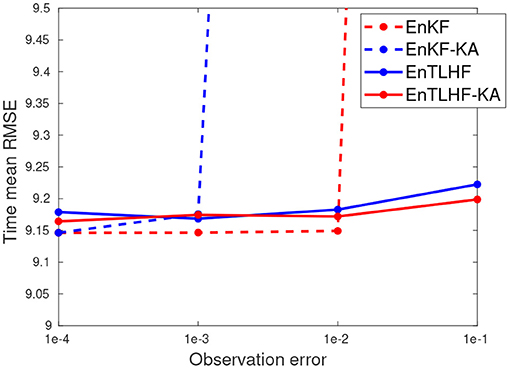
Figure 2. Error evaluation of the robust and non-robust methods with respect to the observation error.

3.3. Robustness Against Model Errors

To evaluate the EnTLHF-KA robustness with respect to model errors, we compare the method's performance when F ∈ [6, 7, 8, 9, 10]. F = 8 corresponds with the assumption of a perfect model. Figure 3 presents the RMSE value for each F value and the comparison among the four filters. The RMSE values remain almost constant for both robust filters, with smaller values for the EnTLHF-KA. The adaptive inflation makes the analysis covariance matrix larger in the robust filters than in its non-robust counterpart, given the same background covariance. Consequently, the EnTLHF and the EnTLHF-KA put more weight in the observations, convenient when there are larger model errors.

FIGURE 3

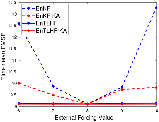
Figure 3. Error evaluation of the robust and non-robust methods with respect to errors in the model.

3.4. Robustness Against Ensemble Distribution

The standard EnKF assumes that the ensemble state has a Gaussian distribution. This assumption is especially essential because the state covariance B is approximated by the ensemble sample covariance P^b. Although the ensemble at t₀ is Gaussian, non-linearities in the model dynamics can modify the ensemble distribution, causing the approximation of B by P^b to lose accuracy. Figure 4 presents an evaluation of the ensemble distribution for different times steps using the Lorenz-96 model. We use the Shapiro-Wilk to evaluate the Gaussianity of each state variable [45]. We take an initial Gaussian ensemble of 100 members as a reference. After 15-time steps, some variables begin to change their initial distribution, and after 30-time steps, the Gaussian assumption is not valid anymore for the ensemble.

FIGURE 4

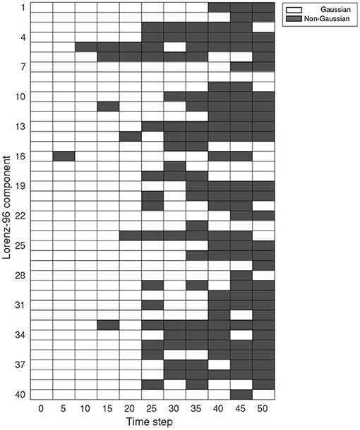
Figure 4. Shapiro-Wilk test for each Lorenz component at a different time step. The ensemble size is 100. The white color represents that the null-hypothesis is not rejected (the ensemble for that specific variable is Gaussian). The gray color represents that the null-hypothesis is rejected (the ensemble for that specific variable is non-Gaussian).

We perform different experiments varying the observation frequency or the number of time steps between two available observations. Figure 5 shows the time averaged RMSE for the EnKF, EnKF-KA, EnTLHF, and the EnTLHF-KA using an observation frequency f ∈ [1, 5, 10, 20, 30, 50] times steps. We set an ensemble size of N = 20, an observation error of δ = 1 × 10⁻³, and the external force F = 8. The EnKF performance decreases considerably when f increases, and after the value of f = 30 the method diverges. This result illustrates the importance of the Gaussian distribution for obtaining a good representation of B throw P^b. The adaptive inflation increases EnTLHF robustness and performance, even when both EnKF and EnTLHF are using the same approximation of B. Nevertheless, the EnTLHF performance decreases considerably when f = 50. In contrast, EnKF-KA and EnTLHF-KA use a shrinkage-based estimator for B. The KA estimator does not assume a Gaussian distribution, as other shrinkage-based estimators do [27, 46]. Thus, the EnKF-KA presents better performance than EnKF for large f values and similar error levels than EnTLH without incorporating adaptive inflation. In the case of the EnTLHF-KA, the combination of both the shrinkage-based estimator and the adaptive inflation produces high robustness and performance even when the ensemble distribution is non-Gaussian.

FIGURE 5

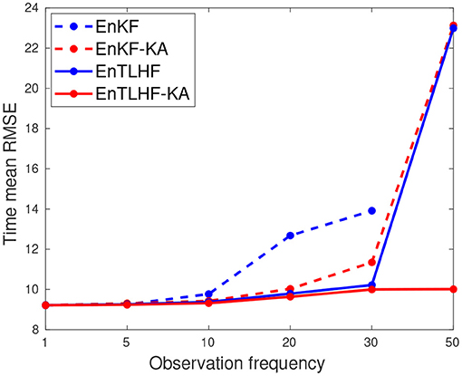
Figure 5. Error evaluation of the robust and non-robust methods with respect to the observation frequency.

4. Application to a Non-linear Non-Gaussian Large Scale System

The implementation of the LOTOS-EUROS CTM over the Aburrá Valley is used as a real study case. This application consists of a non-linear and non-Gaussian large system, so it is a good opportunity to test the proposed method potential. The complete implementation and observations description is presented in the Appendix. The period of interest for all data evaluations, simulations, and DA experiments spans from February 25 to March 15, 2019. During these days, the PM concentrations are higher due to the Northbound transit of the Inter-Tropical Convergence Zone over the study domain. The data to be assimilated is located at the surface but the proposed method also applies to satellite data at different scales and resolutions.

In order to test the proposed method, we performed a total of four different LOTOS-EUROS simulations:

1. a LOTOS-EUROS model simulation without DA (henceforth LE) for having a free run model under regular initial and boundary conditions looking for further comparison;

2. a DA simulation using the LETKF introduced in section 2.1 (henceforth LE-LETKF);

3. a DA simulation using the shrinkage-based EnKF-KA developed in Lopez-Restrepo et al. [15] (henceforth LE-KA);

4. a DA simulation using the robust and shrinkage-based EnTLHF-KA proposed in 2.5 (henceforth LE-Robust).

The set of validation sites is split into two groups: the stations located in the bottom part of the valley (BS, represented by circles in Figure 12), and the stations located in the city's outskirts or hills (OS, represented by stars in Figure 12). The objective of this division is to evaluate the simulation performance in regions where the PM_2.5 concentration regimes are different. All the simulations were evaluated using both validation station's sets, and the performance metrics Mean Fractional Bias (MFB) [47], Root Mean Square Error (RMSE) [48], and Pearson Correlation Factor [49]. The three ensemble-based algorithms estimate both concentrations and emissions, following the stochastic representation presented in Lopez-Restrepo et al. [19]. For all the methods, an ensemble size N of 25 members and a localization radius r of 5 km were used.

The DA methods are evaluated with forecast experiments, in which a model simulation over a limited number of days is performed using information from the assimilation. Forecasting experiments were performed to test the model's capability to predict the PM concentrations in the valley up to three days ahead. We applied the methodology proposed by Lopez-restrepo et al. [50], with all days from March 9 to 13 having predictions as the first, second, and third day of a forecast. We are especially interested in evaluating the ability of the model to predict warning-triggering episodes (AQI in orange, red, or purple levels, as shown in Table 1). All forecast simulations used the estimated emission correction factors from the last assimilation day, in each of the three forecast days. This inheritance scheme has shown the best option for the LE implementation over the Aburrá Valley [19].

TABLE 1

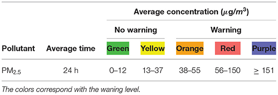
Table 1. Air Quality Index (AQI) as defined for the Aburrá Valley with respect to PM_2.5 concentrations according to the ranges established by the Metropolitan Area.

This is specially relevant in the sense that the robust method is evaluated in the forecast, enhancing the capability of reducing uncertainty in an operational fashion and direct implementation for decision making within our applied research programs in air pollution.

4.1. Target Matrix

The shrinkage-based algorithm EnKF-KA and the robust EnTLHF-KA were implemented to be used with the LOTOS-EUROS model. This was mainly aimed by the fact that there are great opportunities for DA applied to CTM models and air pollution scenarios for decision making. The challenging the problem, the creative solutions arise. The aim of EnKF-KA and the robust EnTLHF-KA algorithms is to improve the model representation in the complex orography conditions of the Aburrá Valley. Both shrinkage-based algorithms required a target matrix T_KA to compute the covariance matrix B according to Equation (10). The matrix T_KA should guide the covariance structure in B by limiting the spurious correlations between elements at a large distance [40], or in the case of the EnKF-KA and the EnTLHF-KA, to incorporate previously obtained knowledge directly in the DA process [15]. For this application, we are interested in using the target matrix to represent the valley's complex orography in the covariance estimation. Previous works have shown issues reproducing the pollutant dynamics into the Aburrá valley due to the limited representation of the valley in the simulation model [19, 21]. Even with high-resolution meteorological simulations, it is still challenging to capture the transport of pollutants in the narrow valleys [51].

The main purpose of the T_KA matrix is to reduce the covariance between elements in the state that are distant in the vertical direction but close in the horizontal direction. Thus, observations located in the bottom part of the valley (where the pollutant concentration are higher) should not have a high impact in the city's outskirts (where the concentrations are lower) and vice versa. A first version of the target matrix ${\text{T}}_{KA}^{*}$ was built using a fourth-order-polynomial covariance function as described in Gaspari and Cohn [44]. To incorporate the previous knowledge and improve the valley representation into the model, we reduced the correlation as a function of vertical distance, with zero correlation for vertical distances exceeding 600 m. Other distances were tested too, without significant changes in the result. The chosen formulation preserves the dependency on the horizontal distance that is necessary to remove the spurious correlations and incorporates the physical restriction of the valley. To ensure that T_KA is positive semidefinite, we applied the method presented in Higham [52] to obtain the positive semidefinite matrix that is closest to ${\text{T}}_{KA}^{*}$ in the Frobenius norm. Figure 6 illustrates the influence area of the Gaspari-Cohn based covariance matrix, the ${\text{T}}_{KA}^{*}$ covariance matrix, and the T_KA covariance matrix for two locations. The influence area corresponds with a row (or column) of the covariance matrix. It is possible to see how the proposed ${\text{T}}_{KA}^{*}$ matrix (Figure 6C) follows the valley shape according to the orography shown in Figure 6B unlike the Gaspari-Cohn covariance matrix (Figure 6A). The generalization applies to very complex boundary conditions in large scale systems not only for the solution of the differential equations but also for the estimation tasks of the robust filters. Additionally, there are no significant modifications between the T_KA (Figure 6D) and the ${\text{T}}_{KA}^{*}$ matrix. Finally, the T_KA matrix is used as the target matrix for both EnKF-KA and EnTLHF-KA methods. Note that the final covariance between the state inside and outside the valley will not be necessary zero because the final covariance matrix B_KA is a convex combination of T_KA and P^b.

FIGURE 6

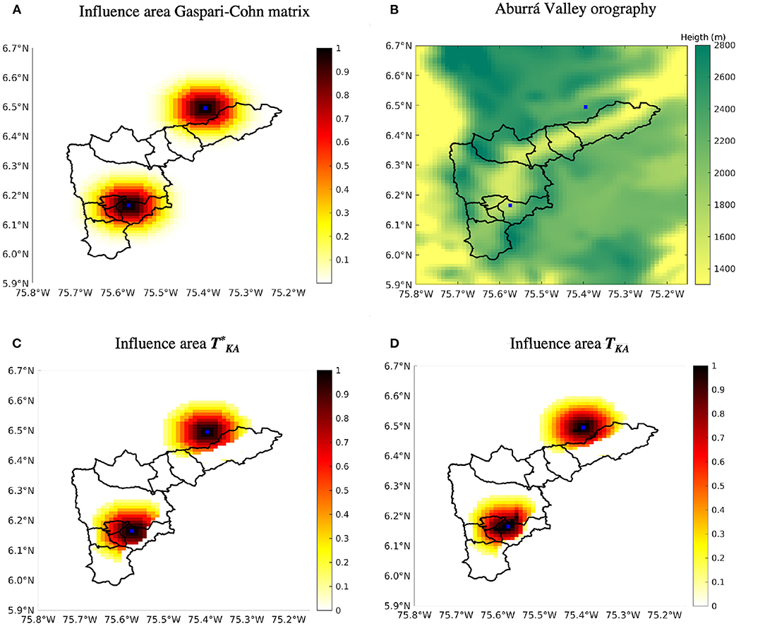
Figure 6. Comparison of the influence area of two selected states (blue dots) between a distance depending localization, and the target covariance matrix based on the distance and the orography. (A) Influence area Gaspari-Cohn matrix. (B) Aburra Valley orography. (C) Influence area ${\text{T}}_{KA}^{*}$. (D) Influence area T_KA.

4.2. Evaluation of LE simulations

The concentration fields produced by model simulations with or without DA were compared with the observations from official monitoring stations (Figure 12), dividing the study into stations at the bottom of the valley (BS stations) and stations at the outskirts of the city (OS stations). The averaged assessment statistics over the validation station are shown in Table 2. In all validation stations, the simulation results without DA (LE) underestimated the observed concentrations. This is for example reflected in a high RMSE value. The correlation coefficient was low, which means that the model could not fully capture the temporal variations at hourly and daily scales. The three simulations using DA had MFB values similar to 0 for the BS stations (bottom of the valley), without a noticeable difference. DA was thus successful in reducing the discrepancy between the model and observations. The RMSE also decreased by 45.03% in the LE-LETKF, 41.57% in the LE-KA, and 41.91% in the LE-Robust simulations compared to the RMSE of the LE simulation. According to Mogollón-sotelo et al. [53], Table 2 based on EPA [54] and Boylan and Russell [47], the R values were all above the criterion for good results. In contrast, over the OS stations (outskirts of the city), the simulations using the shrinkage-based methods presented better statistics compared to the LE-LETKF. For instance, the RMSE's improvements in OS stations using shrinkage-based methods are 15.02% for the LE-KA and 22.22% for the LE-Robust compared with the LE-LETKF.

TABLE 2

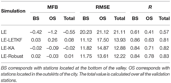
Table 2. Statistical evaluation of different simulations.

TABLE 3

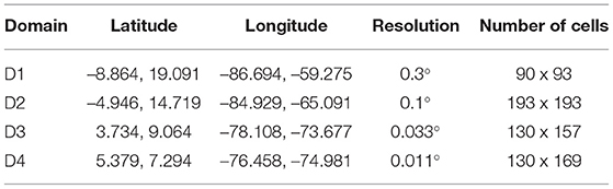
Table 3. Weather research forecast model (WRF) model domains description.

TABLE 4

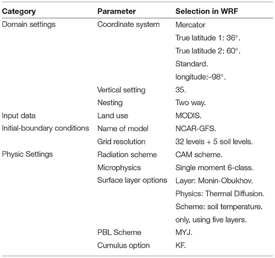
Table 4. WRF model set up.

In general, all DA simulations showed lower scores in the OS stations than in the BS stations, mainly because of the poor representation in these areas by the background simulation (LE simulation) and the lack of close observations. Even so, the LE-Robust looks more robust among all the stations.

Figure 7 shows diurnal cycles in the four chosen validation stations during the simulation phase. Those stations illustrate the differences between BS and OS, and are representative of all validation stations. The LE diurnal cycle differs from the observations in magnitude in the BS stations, and in the OS stations in both magnitude and temporal behavior. The highest peak of concentration in the BS stations around 09:00 is primarily due to traffic dynamics and is partially captured by the LE simulation. For example, the LE morning peak emerged faster in the simulations at station 44 than in the observations. This time lag could be due to a poor spatial representation of mobile sources in the emission inventory, or a failure by the meteorology or the model to reproduce the dynamics of the valley, indicating premature transport of particulate matter to these regions. In comparison, at 22:00 h, the LE simulation presents the highest point at station 44 (Figure 7C), which does not correspond with the observations. The LE simulation in the other OS station 85 (Figure 7D), cannot fit the observation interval, indicating a late morning peak and a minimum around 21:00 that does not appear in the measurements. The LE simulation shows a general underestimation of concentrations, with a better replication of the PM2.5 dynamics at the bottom of the valley.

FIGURE 7

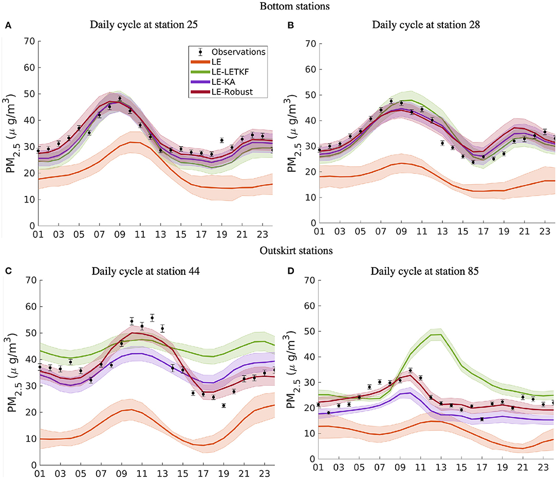
Figure 7. Daily cycle at different stations. The upper panel corresponds with stations located at the bottom of the valley. The bottom panel corresponds with stations located on the outskirts of the city. (A) Daily cycle at station 25. (B) Daily cycle at station 28. (C) Daily cycle at station 44. (D) Daily cycle at station 85.

The simulations using DA presented diurnal cycles closer to the observations, with a marked difference in performance between BS stations and OS stations. In the BS stations (Figures 7A,B), the three methods showed very similar daily cycles capturing the magnitude and the variability of the observations with high accuracy. These simulations corrected the concentration underestimation presented in the LE simulation and improved the temporal profile. Unlike in the BS stations, in the OS stations, the three DA methods showed different results.

The LE-LETKF tends to overestimate the concentrations and has different diurnal variability concerning the observations. In station 44, the LE-LETKF persistently displayed higher values than the observed, and a low variability around the day, with small peaks and valleys. In station 85, the LE-LETKF showed higher concentration values than the observations, and the morning peak appears later (similar to the LE simulation). The discrepancy in the magnitude and the lack of representation of the temporal variability suggest that the LE-LETKF simulation assimilates observations located in regions where the PM presents a different temporal behavior than those grid cells located in the outskirts.

On the other hand, the two simulations using the shrinkage-based covariance estimator and the target matrix T_KA (LE-KA and LE-Robust) improve the performance in the OS stations. The LE-KA simulation showed a similar temporal variability in both OS stations, although a concentration underestimation.

The LE-Robust displayed a high agreement between the simulated daily cycle and the observations. The difference in magnitude between the LE-Robust and LE-KA simulations can be explained by the fact that the robust methods tend to put more weight in the observations when there is high uncertainty in the background [7], such as the case in this application. Finally, the shrinkage-based simulations tend to follow the diurnal variability, which suggests that the T_KA matrix could limit the influence of observations from areas with a different temporal profile.

4.3. Spatial Distribution

To better understand the influence of the target matrix T_KA on shrinkage-based methods, it is important to analyze the spatial distribution of the concentrations over the valley. Figure 8 shows a three-dimensional representation of the average value of PM_2.5 over March 9. In these graphs, values less than 5 μg/m³ are omitted. The averaged observed values are shown using the same color bar for all the validation stations by a circle and a star for the BS and OS stations, respectively.

FIGURE 8

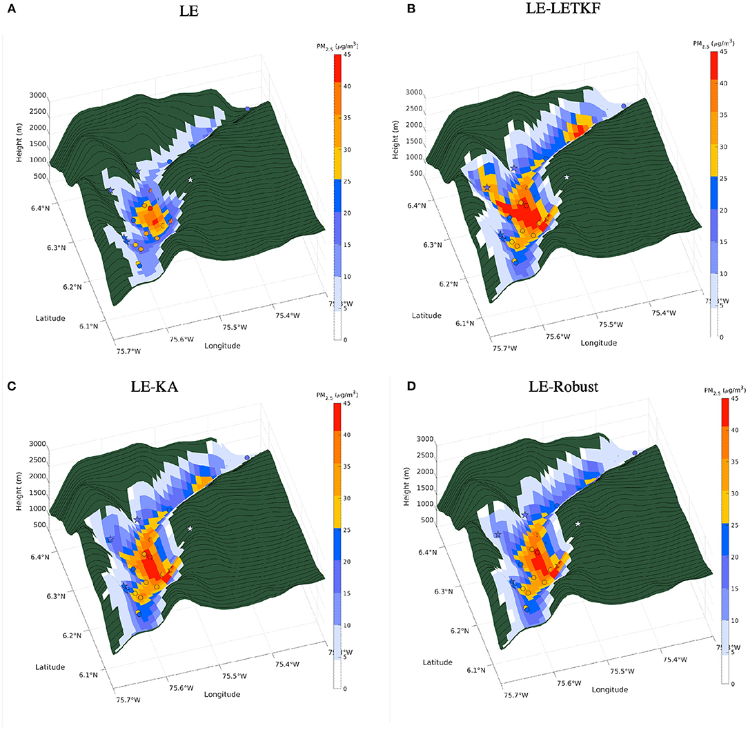
Figure 8. 3D maps of concentrations averaged over March 9 for different simulations. The values less than 5 μg/m³ are omitted. The circles correspond with BS stations, and the stars correspond with OS stations. (A) LE, (B) LE-LETKF, (C) LE-KA, and (D) LE-Robust.

The LE simulation has a spatial pattern similar to the observations, with the highest concentrations in the center and south part of the Medellín city (refer to Figure 12 for reference). In general, the concentrations are higher in the bottom part of the valley, where most of the population and industry facilities are located. This characteristic is well captured by the LE simulation. Nevertheless, the LE simulation tends to underestimate the concentration along the valley and the hills.

The three DA simulations are able to correct the concentration bias in the bottom part of the valley. The LE-LETKF assimilation increases the concentrations in the hills to values higher than the observations. In station 85, located on the west slope of the valley (see Figure 12 for reference), the concentrations simulated by LE-LETKF are almost everywhere higher than the observed. This is because the concentrations in the west hill are influenced by observations located in the lower part of the valley, characterized by high concentrations. Those observations influence the grid cells located on the hill, generating values that do not correspond to the validation station. Both shrinkage-based simulations match better with the observations on the hills. In the case of station 85, both methods have the same range of values as the observed concentrations.

The use of the T_KA matrix limits the influence of the observations located at the bottom of the valley on the grid cells at the slopes. As shown in Figure 6D, the influence of the observations is limited by horizontal and vertical distance, representing better the dynamics in the valley. A particular situation is observed at station 94 (see Figure 12 for reference), located on the top of the east slope. Although the observed values are in the range of 5–10 μg/m³, all the simulations, even the DA simulations, show values under 5 μg/m³ (not plotted in Figure 8). The underestimation can be explained by an absence of emissions in the emission inventory (emission uncertainties), and the limited number of observations in that part of the domain.

4.4. Forecast Results

A fundamental prerequisite for a simulation and assimilation method of air quality to be valuable for a decision-making process is that it can predict the concentrations a few days in advance. Figure 9 shows examples of forecasts from March 12, 16:00 to March 15, 16:00. As was mentioned previously, the forecast runs are using the emission correction factors estimated between March 10, 16:00 and March 11, 16:00. The LE simulation persistently underestimates the concentrations, as observed in the assimilation window's results. In the BS stations, the three assimilation methods initiate a forecast that is quite close to the observations on the first day and remains with an acceptable similarity in the following two forecast days. As shown in the previous evaluations, the concentrations in the assimilation window are very similar for the three methods in the lower part of the valley. Thus, also the estimated emission correction factors are similar, leading to rather small differences between the forecasts. However, in the OS stations, the LE-LETKF forecasts show magnitudes and a temporal behavior that is different from the observations. This discrepancy in the values suggests an incorrect estimation of the emission correction factors on the slopes of the valley by LE-LETKF. The forecasts generated by the shrinkage-based methods are more similar to the observations. The LE-KA and LE-Robust show a good forecasting skills for the OS stations, with temporal behavior and magnitudes close to those observed for the first and second forecast days.

FIGURE 9

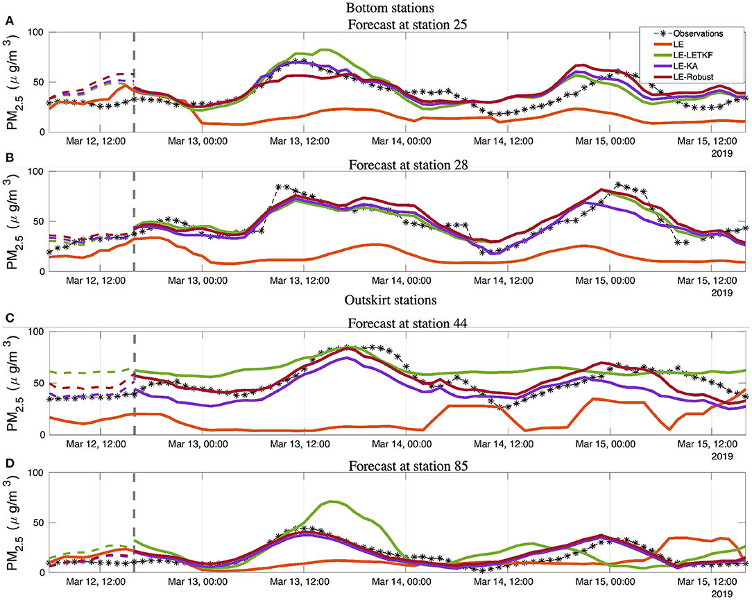
Figure 9. Forecast from March 12, 16:00 to March 15, 16:00 at different stations. The gray vertical dashed line represents the end of the assimilation window and the beginning of the forecast window. Bottom station (A) Forecast cycle at station 25. (B) Forecast cycle at station 28. Outskirt stations (C) Forecast cycle at station 44. (D) Forecast cycle at station 85.

To be valuable for the public, a forecast should correctly warn for elevated air pollution events. The portion of true negatives, true positives, false negatives, and false positives regarding the prediction of warning-triggering episodes (AQI in orange, red, or purple levels, see Table 1) is summarized by the confusion matrix [55].

Figure 10 shows the confusion matrices for LE-LETKF, LE-KA, and LE-Robust assimilations and forecasts. In the assimilation or forecast window, the LE simulation did not give an alert at any station; for that reason, we do not provide its confusion matrix. DA simulations have a ratio between true negatives and true positives equal to or greater than 90% of the 20 alarms registered in the assimilation window, 18 correspond to BS stations.

FIGURE 10

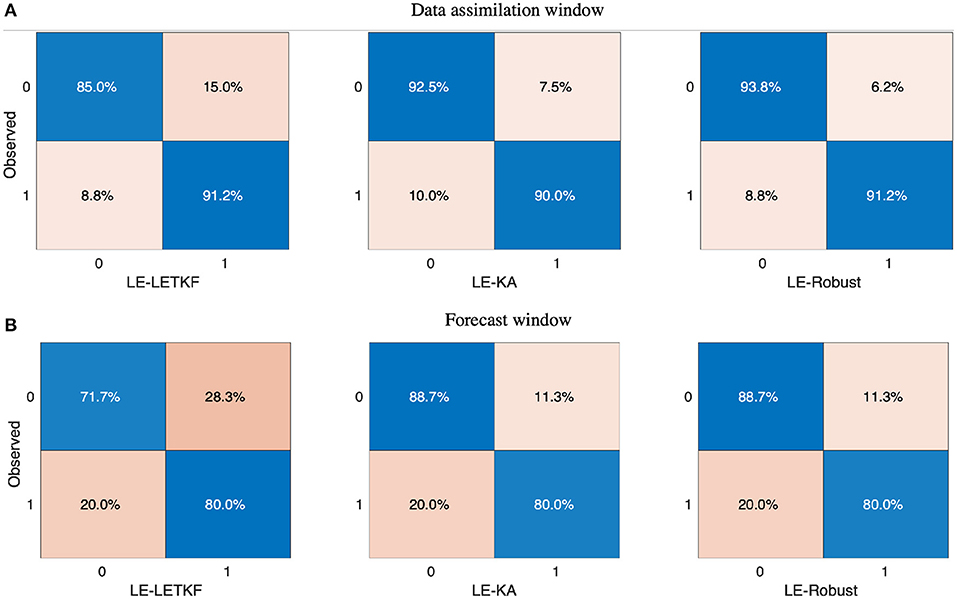
Figure 10. Comparison of confusion matrices for the data assimilation (DA) and forecast window depending on warning or no warning per station. The values are calculated across all the days of the corresponding window. The value of 0 corresponds with no warning, the value of 1 corresponds with a warning. For the LE simulation, there are neither warnings in the DA window nor forecast windows (A,B).

FIGURE 11

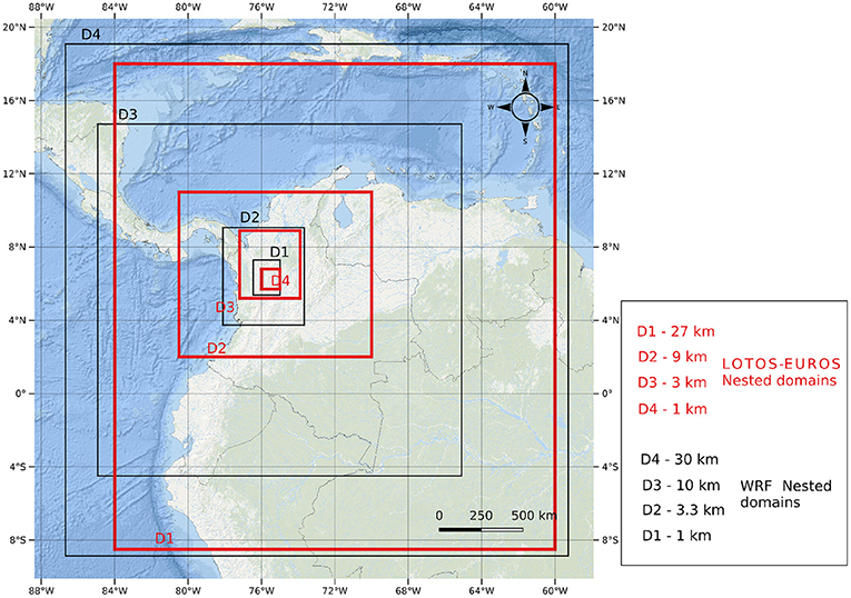
Figure 11. WRF and LOTOS-EUROS model nested domain configuration. The red squares correspond with the LOTOS-EUROS domains, the black squares correspond with the WRF domains.

FIGURE 12

Figure 12. (A) Validation network. The circles and stars represent the bottom part stations (BS), and the outskirt stations (OS), respectively. (B) Assimilation network. The gray raster corresponds with the LOTOS-EUROS model grid, and the black lines are the municipalities, borders.

In the forecast window, the forecast skill of the three models was lower than in the assimilation window. From the 10 actually observed alerts in the forecast period, the DA simulations could replicate 8. A higher proportion of false-positive alerts was reported by the LE-LETKF, documenting nine false alerts more than the shrinkage-based approaches. The high amount of false-positive alerts is due to the overestimation of the LE-LETKF concentration in the OS stations, where the additional alerts were recorded incorrectly. In general, the LE-KA and LE-Robust simulations had better alert forecast performance than the LE-LETKF simulation.

4.5. Discussion and Comments

In a free run scenario for a CTM model, the LOTOS-EUROS model has served as an example for some contributions. Previous studies already suggested the need for meteorological fields at a higher resolution to correctly represent the dynamics and transport of pollutants in the Aburrá Valley [19]. Simulation without DA and using weather research forecast Model (WRF) meteorology (LE simulation) shows an improvement compared to implementations using the lower resolution ECMWF meteorology. This procedure improves the model performance. An underestimation of PM_2.5 concentrations is strongly reduced (although still present) and an increment in the correlation is observed. It is important to continue evaluating the model's performance with different configurations of the WRF model, specifically to reproduce the dominant dynamics of pollutant transport in inhabited valleys [21, 51]. Additionally, it is necessary to carry out a more exhaustive evaluation of the model's vertical resolution, given the new possibilities offered by the coupling with the WRF model. Finally, a reduction in meteorology's uncertainty will improve the estimation of the emissions using DA and could help to create more accurate emission inventories. Data assimilation for uncertainty reduction of the WRF model is under research.

The DA considerably improves the simulations by the model. With each of the three assimilation methods, smaller differences and higher similarities between the simulated and observed concentrations were found, as shown in Table 2. The standard metrics that are used to compare the various algorithms showed an improvement compared to previous EnKF implementations, assimilating the same observations [50]. This improvement is due to the better background obtained using WRF meteorology and the impact of the localization schemes present in the DA algorithms. Using the new assimilation schemes, the spatial distribution of concentrations within the valley is better resolved.

Under the assumption the WRF meteorological fields are on a basis improving the model representation of reality, we will focus on the main differences between the model in a free run and the assimilation. Using a target covariance matrix to adapt the covariances computed from the ensemble results in better representation of the actual covariance structure. The target covariance matrix limits the influence of observations located in the lower part of the valley on the grid cells located in the hills of the valley and vice versa. This makes it possible to separate the different regimes and avoids incorrect corrections in concentrations, as could occur with the standard LEKTF method. The forecast experiments also suggest a better estimate of the emission correction factors when shrinkage methods are employed. As a result, the forecasts of dangerous pollution levels is improved in all the stations (shown in Figure 10). These results encourage further improvement of these types of methods and to incorporate more and more prior knowledge in the covariance estimation. Possible new directions include dynamic target matrices dependent on the weather or on patterns in public behavior.

Both shrinkage-based methods, EnKF-KA and EnTLHF-KA, showed lower error statistics than the standard LETKF. The use of the shrinkage estimator and the incorporation of orography information through the T_KA matrix allows both methods to achieve satisfactory results with a relatively low number of ensemble members (25). Previous experiments in toy models (Lorenz96 and 2D advection-diffusion model) and real pseudo applications (SPEEDY model) have shown that the shrinkage-based family of methods can improve DA when the size of the ensemble is small [15, 40], supported by our results in a real high-dimensional application. This capability is important given the computational difficulty involved in generating many simulations of highly complex models. Although the overall performance of both methods is similar, the robust method achieves better results, especially in stations on the slopes of the valley. This is very important for this family of models because it seems to improve estimation results even if the solution of the differential equation may not be deeply accurate.

The EnTLHF-KA algorithm tends to put more weight on the observations than the EnKF-KA in the analysis step due to the adaptive inflation term that is present. Additionally, the robust methods do not require a completely correct characterization of the observation representation errors or the uncertainties of the model [7]. This characteristic benefits the EnTLHF-KA in our application, given the lack of precise information on the modeling system's uncertainties, e.g., emissions inventory, meteorology, composition, and reaction schemes.

Although the methods presented in this work were tested in a specific setting, their formulation is quite general and could be used in other applications [15]. The basic concept of both EnKF-KA and EnTLHF-KA is to incorporate information or prior system knowledge that is not captured by the model directly in the DA.

In our case, for example, this principle works as a modification to the well-known concept of distance-based location. Several works have followed this line, mainly in history matching applications [56, 57] but with a different approach. We believe that EnKF-KA and EnTLHF-KA possess sufficiently interesting characteristics to be applied and tested in areas other than that shown in this work.

5. Conclusion

This study introduces the concept of robustness from control and systems to a family of DA techniques. We aimed to the natural development of a filter's family that not only avoids spurious correlation but also can be generalized, computationally efficient, and very robust inspired in real life complex systems [15, 19]. We developed the intuition for adding the H_∞ robustness to a shrinkage-based estimator finding a simple and very understandable solution. Using a low-scale model implementation, easily extendable for example to biological systems [58–60] or closed loop estimators for biotechnological process [61, 62], we compared the proposed method's robustness and performance against the standard EnKF, the shrinkage-based EnKF-KA, and the robust filter EnTLHF. The EnTLHF-KA has lower RMSE values in conditions with high observation error and model errors than the other methods. When the number of ensembles is small, the shrinkage estimator gives a better approximation of the background covariance matrix than the sample covariance matrix, generating lower errors in both shrinkage-based algorithm, especially in the EnTLHF-KA. The combination of the non-Gaussian shrinkage estimator and the adaptive inflation grant a higher robustness to the EnTLHF-KA when the ensemble distribution is non-Gaussian.

Additionally , we presented an application using the chemical transport model LOTOS-EUROS over a densely populated valley. The proposed method outperform the standard LETKF, especially in places with complex orography. Incorporating the orography characteristics in the DA through a target matrix, limits the influence of observations in grid cells that are far away in vertical distance. The final result can be understood as a localization scheme that does not depend only on the horizontal distance, but also on the change in orography. The robustness of the EnTLHF-KA allows having a high similarity between the simulated and observed PM_2.5 concentrations, even with a small ensemble size and an incomplete representation of the system uncertainties. The model's forecasting capabilities are also improved, achieving a good representation of the concentrations on the first forecast day, being acceptable until the third day. After assimilation, the model is an accurate tool for forecasting alerts for high levels of air pollution.

Data Availability Statement

The original contributions presented in the study are included in the article/supplementary material, further inquiries can be directed to the corresponding author/s.

Author Contributions

SL-R: conceptualization, methodology, software, and writing—original draft. AY: methodology and software. NP: conceptualization, methodology, writing—review, and editing. OQ: conceptualization, methodology, writing—original draft, editing, and supervision. AS: methodology, software, writing—review, and editing. AH: writing—review, editing, and supervision. All authors have read and agreed to the published version of the manuscript.

Conflict of Interest

SL-R and AY were employed by the company SimpleSpace.

The remaining authors declare that the research was conducted in the absence of any commercial or financial relationships that could be construed as a potential conflict of interest.

Publisher's Note

All claims expressed in this article are solely those of the authors and do not necessarily represent those of their affiliated organizations, or those of the publisher, the editors and the reviewers. Any product that may be evaluated in this article, or claim that may be made by its manufacturer, is not guaranteed or endorsed by the publisher.

Acknowledgments

The authors acknowledge the supercomputing resources made available by the Centro de Computación Científica Apolo at Universidad EAFIT (http://www.eafit.edu.co/apolo) to conduct this work.

Abbreviations

DA, Data Assimilation; KF, Kalman Filter; EnKF, ENsemble Kalman Filter; LETKF, Local Ensemble Transform Kalman Filter; KA, Knowledge-Aided; EnKF-KA, Ensemble Kalman Filter Knowledge-Aided; HF, H_∞ Filter; EnTLHF, ENsemble Time Local H_∞ Filter; EnTLHF-KA, ENsemble Time Local H_∞ Filter Knowledge-Aided; RMSE, Root Mean Square Error; CTM, Chemical Transport Model; LE, LOTOS-EUROS simulation without data assimilation; LE-LETKF, LOTOS-EUROS simulation using the LETKF; LE-KA, LOTOS-EUROS simulation using the EnKF-KA; LE-Robust, LOTOS-EUROS simulation using the EnTLHF-KA; BS, Bottom Stations; OS, Outskirts Stations.

References

1. Lahoz WA, Schneider P. Data assimilation: making sense of earth observation. Front Environ Sci. (2014) 2:16. doi: 10.3389/fenvs.2014.00016

CrossRef Full Text | Google Scholar

2. Bocquet M, Elbern H, Eskes H, Hirtl M, Aabkar R, Carmichael GR, et al. Data assimilation in atmospheric chemistry models: current status and future prospects for coupled chemistry meteorology models. Atmosphere Chem Phys. (2015) 15:5325–58. doi: 10.5194/acp-15-5325-2015

CrossRef Full Text | Google Scholar

3. Kalman RE. A new approach to linear filtering and prediction problems. J Basic Eng. (1960) 82:35–45. doi: 10.1115/1.3662552

PubMed Abstract | CrossRef Full Text | Google Scholar

4. Evensen G. The ensemble kalman filter: theoretical formulation and practical implementation. Ocean Dyn. (2003) 53:343–67. doi: 10.1007/s10236-003-0036-9

CrossRef Full Text | Google Scholar

5. Houtekamer PL, Mitchell HL, Pellerin G, Buehner M, Charron M, Spacek L, et al. Atmospheric data assimilation with an ensemble kalman filter: results with real observations. Mon Weather Rev. (2005) 133:604–20. doi: 10.1175/MWR-2864.1

CrossRef Full Text | Google Scholar

6. Bai Y, Zhang Z, Zhang Y, Wang L. Inflating transform matrices to mitigate assimilation errors with robust filtering based ensemble Kalman filters. Atmosphere Sci Lett. (2016) 17:470–8. doi: 10.1002/asl.681

CrossRef Full Text | Google Scholar

7. Luo X, Hoteit I. Robust ensemble filtering and its relation to covariance inflation in the ensemble kalman filter. Mon Weather Rev. (2011) 139:3938–53. doi: 10.1175/MWR-D-10-05068.1

CrossRef Full Text | Google Scholar

8. Han Y, Zhang Y, Wang Y, Ye S, Fang H. A new sequential data assimilation method. Sci China E Technol Sci. (2009) 52:1027–38. doi: 10.1007/s11431-008-0189-3

CrossRef Full Text | Google Scholar

9. Nan TC, Wu JC. Application of ensemble H-infinity filter in aquifer characterization and comparison to ensemble Kalman filter. Water Sci Eng. (2017) 10:25–35. doi: 10.1016/j.wse.2017.03.009

CrossRef Full Text | Google Scholar

10. Roh S, Genton MG, Jun M, Szunyogh I, Hoteit I. Observation quality control with a robust ensemble kalman filter. Mon Weather Rev. (2013) 141:4414–28. doi: 10.1175/MWR-D-13-00091.1

CrossRef Full Text | Google Scholar

11. Freitag MA, Nichols NK, Budd CJ. Resolution of sharp fronts in the presence of model error in variational data assimilation. Q J R Meteorol Soc. (2013) 139:742–57. doi: 10.1002/qj.2002

CrossRef Full Text | Google Scholar

12. Rao V, Sandu A, Ng M, Nino-Ruiz ED. Robust data assimilation using l1 and huber norms. SIAM J Sci Comput. (2017) 39:B548–70. doi: 10.1137/15M1045910

CrossRef Full Text | Google Scholar

13. Yang Y, He H, Xu G. Adaptively robust fitering for kinematic geodetic positioning. J Geodesy. (2001) 75:109–16. doi: 10.1007/s001900000157

CrossRef Full Text | Google Scholar

14. Nino-Ruiz E, Cheng H, Beltran R, Nino-Ruiz ED, Cheng H, Beltran R. A robust non-gaussian data assimilation method for highly non-linear models. Atmosphere. (2018) 9:126. doi: 10.3390/atmos9040126

CrossRef Full Text | Google Scholar

15. Lopez-Restrepo S, Nino-Ruis ED, Yarce A, Quintero OL, Pinel N, Segers A, et al. An efficient ensemble kalman filter implementation via shrinkage covariance matrix estimation: exploiting prior knowledge. Comput Geosci. (2021) 25:985–1003. doi: 10.1007/s10596-021-10035-4

CrossRef Full Text | Google Scholar

16. Fu G, Prata F, Xiang Lin H, Heemink A, Segers A, Lu S. Data assimilation for volcanic ash plumes using a satellite observational operator: a case study on the 2010 Eyjafjallajökull volcanic eruption. Atmosphere Chem Phys. (2017) 17:1187–205. doi: 10.5194/acp-17-1187-2017

CrossRef Full Text | Google Scholar

17. Lu S, Lin HX, Heemink A, Segers A, Fu G. Estimation of volcanic ash emissions through assimilating satellite data and ground-based observations. J Geophys Res. (2016) 121:971–10. doi: 10.1002/2016JD025131

CrossRef Full Text | Google Scholar

18. Jin J, Lin HX, Heemink A, Segers A. Spatially varying parameter estimation for dust emissions using reduced-tangent-linearization 4DVar. Atmos Environ. (2018) 187:358–73. doi: 10.1016/j.atmosenv.2018.05.060

CrossRef Full Text | Google Scholar

19. Lopez-Restrepo S, Yarce A, Pinel N, Quintero OL, Segers A, Heemink AW. Forecasting PM10 and PM2.5 in the Aburrá valley (Medellín, Colombia) via EnKF based data assimilation. Atmos Environ. (2020) 232:117507. doi: 10.1016/j.atmosenv.2020.117507

CrossRef Full Text | Google Scholar

20. Hoyos CD, Herrera-Mejía L, Roldán-Henao N, Isaza A. Effects of fireworks on particulate matter concentration in a narrow valley: the case of the Medellín metropolitan area. Environ Monit Assess. (2019) 192:6. doi: 10.1007/s10661-019-7838-9

PubMed Abstract | CrossRef Full Text | Google Scholar

21. Henao JJ, Mejía JF, Rendón AM, Salazar JF. Sub-kilometer dispersion simulation of a CO tracer for an inter-Andean urban valley. Atmos Pollut Res. (2020) 11:928–945. doi: 10.1016/j.apr.2020.02.005

CrossRef Full Text | Google Scholar

22. Liu C, Xiao Q, Wang B. An ensemble-based four-dimensional variational data assimilation scheme. Part I: technical formulation and preliminary test. Mon Weather Rev. (2008) 136:3363–73. doi: 10.1175/2008MWR2312.1

CrossRef Full Text | Google Scholar

23. Ott E, Hunt BR, Szunyogh I, Zimin AV, Kostelich E, Corazza M, et al. A local ensemble Kalman filter for atmospheric data assimilation. Tellus. (2004) 56:415–28. doi: 10.3402/tellusa.v56i5.14462

PubMed Abstract | CrossRef Full Text | Google Scholar

24. Shin S, Kang JS, Jo Y. The local ensemble transform kalman filter (LETKF) with a global NWP model on the cubed sphere. Pure Appl Geophys. (2016) 173:2555–70. doi: 10.1007/s00024-016-1269-0

CrossRef Full Text | Google Scholar

25. Touloumis A. Nonparametric Stein-type shrinkage covariance matrix estimators in high-dimensional settings. Comput Stat Data Anal. (2015) 83:251–61. doi: 10.1016/j.csda.2014.10.018

CrossRef Full Text | Google Scholar

26. Couillet R, McKay M. Large dimensional analysis and optimization of robust shrinkage covariance matrix estimators. J Multivar Anal. (2014) 131:99–120. doi: 10.1016/j.jmva.2014.06.018

CrossRef Full Text | Google Scholar

27. Ledoit O, Wolf M. Optimal estimation of a large-dimensional covariance matrix under Stein's loss. Bernoulli. (2018) 24:3791–832. doi: 10.3150/17-BEJ979

CrossRef Full Text | Google Scholar

28. Stoica P, Li J, Zhu X, Guerci JR. On using a priori knowledge in space-time adaptive processing. IEEE Trans Signal Process. (2008) 56:2598–602. doi: 10.1109/TSP.2007.914347

PubMed Abstract | CrossRef Full Text | Google Scholar

29. Zhu X, Li J, Stoica P. Knowledge-aided space-time adaptive processing. IEEE Trans Aerospace Electron Syst. (2011) 47:1325–36. doi: 10.1109/TAES.2011.5751261

PubMed Abstract | CrossRef Full Text | Google Scholar

30. Hassibi B, Kailath T, Sayed A. Array algorithms for H estimation. Automatic Control IEEE ldots. (2000) 45:702–6. doi: 10.1109/9.847105

CrossRef Full Text | Google Scholar

31. Wang D, Cai X. Robust data assimilation in hydrological modeling – A comparison of Kalman and H -infinity filters. Adv Water Resour. (2008) 31:455–72. doi: 10.1016/j.advwatres.2007.10.001

CrossRef Full Text | Google Scholar

32. Berger JO. Statistical Decision Theory and Bayesian Analysis. Springer Series in Statistics. New York, NY: Springer (1985).

PubMed Abstract | Google Scholar

33. Anderson JL. An ensemble adjustment kalman filter for data assimilation. Mon Weather Rev. (2001) 129:2884–2903. doi: 10.1175/1520-0493(2001)129<2884:AEAKFF>2.0.CO;2

CrossRef Full Text | Google Scholar

34. Bellsky T, Mitchell L. A shadowing-based inflation scheme for ensemble data assimilation. Physica D. (2018) 380-381:1–7. doi: 10.1016/j.physd.2018.05.002

CrossRef Full Text | Google Scholar

35. Houtekamer PL, Zhang F. Review of the ensemble kalman filter for atmospheric data assimilation. Mon Weather Rev. (2016) 144, 4489–4532. doi: 10.1175/MWR-D-15-0440.1

CrossRef Full Text | Google Scholar

36. Altaf MU, Butler T, Luo X, Dawson C, Mayo T, Hoteit I. Improving short-range ensemble kalman storm surge forecasting using robust adaptive inflation. Mon Weather Rev. (2013) 141:2705–20. doi: 10.1175/MWR-D-12-00310.1

CrossRef Full Text | Google Scholar

37. Triantafyllou G, Hoteit I, Luo X, Tsiaras K, Petihakis G. Assessing a robust ensemble-based Kalman filter for efficient ecosystem data assimilation of the Cretan Sea. J Mar Syst. (2013) 125:90–100. doi: 10.1016/j.jmarsys.2012.12.006

CrossRef Full Text | Google Scholar

38. Sakov P, Bertino L. Relation between two common localisation methods for the EnKF. Comput Geosci. (2011) 15:225–37. doi: 10.1007/s10596-010-9202-6

CrossRef Full Text | Google Scholar

39. Chen Y, Wiesel A, Hero AO. Shrinkage estimation of high dimensional covariance matrices. In: 2009 IEEE International Conference on Acoustics, Speech and Signal Processing. Taipei: IEEE (2009). p. 2937–40.

Google Scholar

40. Nino-ruiz ED, Sandu A. Ensemble Kalman filter implementations based on shrinkage covariance matrix estimation. Ocean Dyn. (2015) 65:1423–39. doi: 10.1007/s10236-015-0888-9

CrossRef Full Text | Google Scholar

41. Nino-Ruiz ED, Sandu A. Efficient parallel implementation of DDDAS inference using an ensemble Kalman filter with shrinkage covariance matrix estimation. Cluster Comput. (2017) 22:1–11. doi: 10.1007/s10586-017-1407-1

CrossRef Full Text | Google Scholar

42. Lorenz EN, Emanuel KA. optimal sites for supplementary weather observations: simulation with a small model. J Atmosphere Sci. (1998) 55:399–414. doi: 10.1175/1520-0469(1998)055<0399:OSFSWO>2.0.CO;2

CrossRef Full Text | Google Scholar

43. Gottwald GA, Melbourne I. Testing for chaos in deterministic systems with noise. Physica D. (2005) 212:100–10. doi: 10.1016/j.physd.2005.09.011

CrossRef Full Text | Google Scholar

44. Gaspari G, Cohn SE. Construction of correlation functions in two and three dimensions. Q J R Meteorol Soc. (1999) 125:723–57. doi: 10.1002/qj.49712555417

CrossRef Full Text | Google Scholar

45. Shapiro S, Wilk M. An analysis of variance test for normality (complete samples)†. Biometrika. (1965) 52:591–611. doi: 10.1093/biomet/52.3-4.591

CrossRef Full Text | Google Scholar

46. Nino-Ruiz ED, Guzman L, Jabba D. An ensemble Kalman filter implementation based on the Ledoit and Wolf covariance matrix estimator. J Comput Appl Math. (2021) 384:113163. doi: 10.1016/j.cam.2020.113163

CrossRef Full Text | Google Scholar

47. Boylan JW, Russell AG. PM and light extinction model performance metrics, goals, and criteria for three-dimensional air quality models. Atmos Environ. (2006) 40: 4946–59. doi: 10.1016/j.atmosenv.2005.09.087

CrossRef Full Text | Google Scholar

48. Chai T, Draxler RR. Root mean square error (RMSE) or mean absolute error (MAE): arguments against avoiding RMSE in the literature. Geosci Model Dev. (2014) 7:1247–50. doi: 10.5194/gmd-7-1247-2014

CrossRef Full Text | Google Scholar

49. Yu S, Eder B, Dennis R, Chu SH, Schwartz SE. New unbiased symmetric metrics for evaluation of air quality models. Atmosphere Sci Lett. (2006) 7:26–34. doi: 10.1002/asl.125

CrossRef Full Text | Google Scholar

50. Lopez-restrepo S, Yarce A, Pinel N, Heemink AW. Urban Air quality modeling using low-cost sensor network and data assimilation in the aburrá valley, colombia. Atmosphere. (2021) 12:1–19. doi: 10.3390/atmos12010091

CrossRef Full Text | Google Scholar

51. Rendón AM, Salazar JF, Wirth V. Daytime air pollution transport mechanisms in stable atmospheres of narrow versus wide urban valleys. Environ Fluid Mech. (2020) 20:1101–18. doi: 10.1007/s10652-020-09743-9

CrossRef Full Text | Google Scholar

52. Higham NJ. Computing a nearest symmetric positive semidefinite matrix. Linear Algebra Appl. (1988) 103:103–18. doi: 10.1016/0024-3795(88)90223-6

CrossRef Full Text | Google Scholar

53. Mogollón-sotelo C, Belalcazar L, Vidal S. A support vector machine model to forecast ground-level PM2.5 in a highly populated city with a complex terrain. Air Qual Atmosphere Health. (2020) 14:399–409. doi: 10.1007/s11869-020-00945-0

CrossRef Full Text | Google Scholar

54. EPA. Meteorological Monitoring Guidance for Regulatory Modeling Applications. Research Triangle Park, NC: U.S. Environmental Protection Agency (2000).

Google Scholar

55. Kohavi R, Provost F. Applications of machine learning and the knowledge. Appl Mach Learn Knowl Mach Learn. (1998) 30:349–54. doi: 10.1023/A:1007442505281

CrossRef Full Text

56. Soares RV, Maschio C, Schiozer DJ. Applying a localization technique to Kalman Gain and assessing the influence on the variability of models in history matching. J Petrol Sci Eng. (2018) 169:110–25. doi: 10.1016/j.petrol.2018.05.059

CrossRef Full Text | Google Scholar

57. Lacerda JM, Emerick AA, Pires AP. Using a machine learning proxy for localization in ensemble data assimilation. Comput Geosci. (2021) 25:11–13. doi: 10.1007/s10596-020-10031-0

CrossRef Full Text | Google Scholar

58. Parra-Amaya ME, Puerta-Yepes ME, Lizarralde-Bejarano DP, Arboleda-Sánchez S. Early detection for dengue using local indicator of spatial association (LISA) analysis. Diseases. (2016) 4:16. doi: 10.3390/diseases4020016

PubMed Abstract | CrossRef Full Text | Google Scholar

59. Lizarralde-Bejarano DP, Arboleda-Sánchez S, Puerta-Yepes ME. Understanding epidemics from mathematical models: details of the 2010 dengue epidemic in Bello (Antioquia, Colombia). Appl Math Model. (2017) 43:566–78. doi: 10.1016/j.apm.2016.11.022

CrossRef Full Text | Google Scholar

60. Catano-Lopez A, Rojas-Diaz D, Laniado H, Arboleda-Sánchez S, Puerta-Yepes ME, Lizarralde-Bejarano DP. An alternative model to explain the vectorial capacity using as example Aedes aegypti case in dengue transmission. Heliyon. (2019) 5:e02577. doi: 10.1016/j.heliyon.2019.e02577

PubMed Abstract | CrossRef Full Text | Google Scholar

61. Quintero OL, Amicarelli AA, Di Sciascio F, Scaglia G. State estimation in alcoholic continuous fermentation of Zymomonas mobilis using recursive bayesian filtering: a simulation approach. BioResources. (2008) 3:316–34.

Google Scholar

62. Quintero OL, Amicarelli AA, Scaglia G, di Sciascio F. Control based on numerical methods and recursive Bayesian estimation in a continuous alcoholic fermentation process. BioResources. (2009) 4:1372–95.

Google Scholar

63. Manders AMM, Builtjes PJH, Curier L, Denier Van Der Gon HAC, Hendriks C, Jonkers S, et al. Curriculum vitae of the LOTOS-EUROS (v2.0) chemistry transport model. Geosci Model Dev. (2017) 10:4145–73. doi: 10.5194/gmd-10-4145-2017

CrossRef Full Text | Google Scholar

64. Skamarock WC, Klemp JB, Dudhi J, Gill DO, Barker DM, Duda MG, et al. A Description of the Advanced Research WRF Version 3. Boulder, CO: University Corporation for Atmospheric Research (2008).

Google Scholar

65. Petrescu AMR, Abad-Vi nas R, Janssens-Maenhout G, Blujdea VNB, Grassi G. Global estimates of carbon stock changes in living forest biomass: EDGARv4.3 - time series from 1990 to 2010. Biogeosciences. (2012) 9:3437–47. doi: 10.5194/bg-9-3437-2012

CrossRef Full Text | Google Scholar

66. Misenis C, Zhang Y. An examination of sensitivity of WRF/Chem predictions to physical parameterizations, horizontal grid spacing, and nesting options. Atmosphere Res. (2010) 97:315–34. doi: 10.1016/j.atmosres.2010.04.005

CrossRef Full Text | Google Scholar

67. Carvalho D, Rocha A, Gómez-Gesteira M, Santos C. A sensitivity study of the WRF model in wind simulation for an area of high wind energy. Environ Model Softw. (2012) 33:23–34. doi: 10.1016/j.envsoft.2012.01.019

CrossRef Full Text | Google Scholar

68. Tuccella P, Curci G, Visconti G, Bessagnet B, Menut L, Park RJ. Modeling of gas and aerosol with WRF/Chem over Europe: evaluation and sensitivity study. J Geophys Res Atmospheres. (2012) 117:1–15. doi: 10.1029/2011JD016302

CrossRef Full Text | Google Scholar

69. Hu XM, Klein PM, Xue M. Evaluation of the updated YSU planetary boundary layer scheme within WRF for wind resource and air quality assessments. J Geophys Res Atmospheres. (2013) 118:10490–505. doi: 10.1002/jgrd.50823

CrossRef Full Text | Google Scholar

70. Dillon ME, Skabar YG, Ruiz J, Kalnay E, Collini EA, Echevarría P, et al. Application of the WRF-LETKF data assimilation system over southern South America: sensitivity to model physics. Weather Forecast. (2016) 31:217–36. doi: 10.1175/WAF-D-14-00157.1

CrossRef Full Text | Google Scholar

71. Kumar A, Jiménez R, Belalcázar LC, Rojas NY. Application of WRF-Chem model to simulate PM10 concentration over Bogotá. Aerosol Air Qual Res. (2016) 16:1206–21. doi: 10.4209/aaqr.2015.05.0318

CrossRef Full Text | Google Scholar

Appendix

The Chemical Transport Model LOTOS-EUROS Setup

The LOTOS-EUROS (LOng Term Ozone Simulation - EURopean Operational Smog) model is a 3D Chemical Transport Model that simulates trace gas and aerosol concentrations in the lower troposphere [63]. The physical processes in the model include emission, advection, diffusion, chemical reactions, and dry and wet deposition. The input to the LOTOS-EUROS model mainly consists of meteorological data, emission inventories, and surface data such as land-use and vegetation type. For a full description of the physical processes and input data could be found [63]. Simulations were conducted with the LE model, adopting a nested domain configuration shown in Figure 11 and following previous implementations [19, 50]. The first Domain (D1) has a model resolution of 0.27° × 0.27°. For this domain, meteorological data from ECMWF was used at a resolution of 0.14° × 0.14°. The inner domain D2 is centered over the valley, encompassing most of the Colombian Andes; the model resolution was set to 0.09° × 0.09°. For this and the following inner domain, meteorological data were obtained from ECMWF at 0.07° × 0.07° resolution. The third inner domain, D3 includes the department of Antioquia, at a model resolution of 0.03° × 0.003°. The innermost domain D4 includes primarily the region of the Aburrá Valley, using the model resolution of 0.01° × 0.01°. The simulations in the domain of interest (D4) were performed using the meteorological fields coming from the Weather Research and Forecasting (WRF) model [64]. The description of the WRF meteorology is presented in Section 25. The anthropogenic emissions for the domains D4, D3, and D2 were obtained from the global EDGAR emission inventory V4.3 [65]. In domain D4, the local emission inventory for particulate matter presented in Lopez-restrepo et al. [50] was used as anthropogenic emissions. For all the domains, the biogenic emissions were obtained from the MEGAN emission inventory and the biomass burning and fires from MACC/CAMS GFAS inventory.

The WRF Meteorology

The WRF model is a numerical weather prediction and atmospheric simulation system designed for research and operational applications [64]. The WRF simulations are suitable to understand the behavior of meteorological variables in a domain like the Aburrá Valley. The WRF model has been used over Colombia in previous studies [21, 66–71]. The configuration of the nested domains used in this study is shown in the Figure 11 and described in Table 3. The settings used for the WRF simulations are summarized in Table 4.

The Data Used for Assimilation and Validation

We used the hyper-dense low-cost network deployed and operated by the Sistema de Alerta Temprana del Valle de Aburrá (SIATA) as observations for the DA methods. The low-cost network consists of 255 real-time PM_2.5 sensors across the Aburrá Valley and its hills. Hoyos et al. [20] presents the description and calibration process of the low-cost sensor. In Lopez et al.'s [50] study, the low-cost sensor networks are evaluated and used as observations for the standard DA method, EnKF, outperforming the simulation where the standard network was used as observations for the same DA method. For validation, we used the independent official monitoring network of the metropolitan area. The official network has 21 measurement sites that observer particulate matter at hourly frequency [20]. The distribution of both observations network is shown in Figure 12.

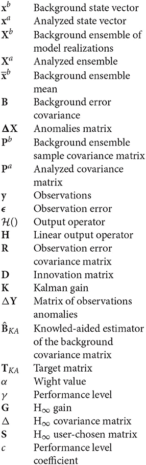
Nomenclature

List of Symbols