GPU Accelerated Parallel Processing for Large-Scale Monte Carlo Analysis: COVID-19 Parameter Estimation and New Case Forecasting

Markov Chain Monte Carlo methods have emerged as one of the premier approaches to estimating posterior distributions for use in Bayesian computations. Unfortunately, these methods often suffer from slow run times when the data become large or when the parameter values come from complex distributions. This speed issue has prevented MCMC analysis from being used to solve some of the most interesting problems for which its technique is a good fit. We used the Multiple-Try Metropolis variant of the basic Metropolis Hastings algorithm, which trades off running more parallel likelihood calculations in favor of a higher acceptance rate and faster convergence compared to traditional MCMC. We optimized our algorithm to parallelize it and to take advantage of GPU processing. We applied our approach to parameter estimation for a Susceptible-Exposed-Infectious-Removed (SEIR) model and forecasting new cases of COVID-19. In comparison to a fully parallelized CPU implementation, using a single GPU to execute the simulations resulted in more than a 13x speedup in wall clock time, running on multiple GPUs resulted in a 36.3x speedup in wall clock time, and using a cloud-based server consisting of 8 GPUs resulted in a 56.5x speedup in wall clock time. Our approach shows that MCMC methods can be utilized to tackle problems that were previously thought to be too computationally intensive and slow.

1. Introduction

This paper explores the use of computer algorithm optimization and parallelization to accelerate large-scale Markov Chain Monte Carlo (MCMC) analyses which were applied to parameter estimation for a Susceptible-Exposed-Infectious-Removed (SEIR) model and forecasting new cases of COVID-19. A large quantity of simulations was run to estimate the parameter values in the SEIR model and increase their accuracy through optimization via graphics processing unit (GPU) processing and parallelization of both the likelihood function and multiple MCMC chains using a multiple-try Metropolis (MTM) MCMC algorithm. The key accomplishment of this project was the application of optimization and parallelization techniques to speed up the MCMC analysis to the point that it could be used in a large, real-world situation, demonstrating that theoretical improvements are now achievable with existing computer hardware, parallel programming, and GPU acceleration.

MCMC methods have emerged as one of the premier approaches to estimating posterior distributions for use in Bayesian computations, which have been useful in a number of fields, including machine learning [1], physics [2], and systems biology [3]. Unfortunately, these methods often suffer from slow run times when the data become large or when the parameter values come from complex distributions. This speed issue has prevented MCMC analysis from being used to solve some of the most interesting problems for which its technique is a good fit. Finding methods to improve the speed while maintaining accuracy without bias has been a topic many researchers have investigated [4, 5]. Other methods have been proposed to improve the convergence rate, resulting in more accurate results for the same number of iterations of the MCMC algorithm [6, 7]. The Multiple-Try Metropolis algorithm is one technique that has arisen that can improve computation speeds through parallel processing because the algorithm itself is highly parallelizable [8]. While parallelizing computations will inevitably reduce computational time, we have sought to increase speed further by optimizing the code to also leverage hardware advances to decrease the time it takes for analysis by running on GPUs.

The idea for the MCMC method used in this example comes from a source-reconstruction plume dispersion model currently in development. This original work takes a time series of chemical concentration signals recorded by field sensors at known locations. It then works backwards from those signals to estimate the most likely source of the chemical release. An MCMC chain is used to run the plume model in a forward direction, and the similarity of the real sensor data to the estimates from the plume model is used as the likelihood function to infer the most likely parameter values that describe the chemical release.

In this paper we instead start with a time series of COVID-19 cases. We then use MCMC to work backward to estimate SEIR parameter values which works in a similar manner plume model case. In both cases, the computation of the likelihood function involves running a complex physics-based simulation in the forward direction and then using the simulation's results to calculate a likelihood. The inclusion of the physics-based simulation in the likelihood function makes it impractical to use any MCMC variants, such as Hamiltonian Monte Carlo, which require the gradient of the likelihood function. At the same time, these particular physics simulations are simple enough that running a single instance of them does not require enough work to fully utilize the hardware of even a single modern GPU.

This creates a particularly challenging problem, because MCMC methods are inherently sequential algorithms. Calculating each step of the chain requires knowing the state of the chain from the previous step as input. This can make them computationally expensive when analyzing large datasets and complex parameter sets, making them impractical in those situations [9]. Many approaches to parallelizing and accelerating MCMC algorithms have been proposed that mainly fall into two categories. One approach is to divide the problem into smaller pieces that can be run independently and in parallel. The other approach is to use knowledge of the posterior, priors or other information to accelerate the convergence rate and reduce the number of iterations required [4, 5]. For example, the simplest of these approaches is to just run several independent chains in parallel and then average the results. Alternatively, one can run multiple interacting chains that share information at certain points in the step to reduce the number of iterations required for convergence. Other methods such as Hamiltonian Monte Carlo (HMC) and No U-Turn Sampling (NUTS) use auxiliary parameters combined with Hamiltonian dynamics and the ability to calculate the likelihood function's gradients to accelerate convergence [10, 11].

Our approach to accelerating the SEIR-based MCMC chains was twofold. First, we used multiple parallel chains that synchronize on each iteration before the next proposal point is drawn. During the drawing of the proposal point, each chain uses the other chain locations as samples to estimate the local parameter covariances. This allows us to use a multivariate Gaussian proposal distribution that more closely estimates the target posterior at each step. Second, we used the MTM variant of the basic Metropolis Hastings (MH) algorithm [8, 12]. The MTM algorithm trades off running more parallel likelihood calculations in favor of a higher acceptance rate, faster convergence, and fewer total iterations compared to traditional MCMC. We then optimized our algorithm to parallelize it from the top down with a synchronization point in the likelihood function just prior to starting the SEIR model simulations. This allowed us to simultaneously launch an entire ensemble of SEIR simulations that need to be run on GPU. The entire ensemble could then be solved in parallel using the fine-grained data parallel execution model of GPUs as opposed to the independent course-grained task parallel model of central processing units (CPUs).

2. Materials and Methods

2.1. Background

2.1.1. SEIR Applications

Prior to this research, IEM had developed a tool (BioSim) that allows users to quickly and efficiently build epidemiological compartment models with any number of compartments and connections, and leverages the computational power of Nvidia GPUs to significantly accelerate solving ensembles of compartment model problems in parallel. The application of this research was to explore methods for applying parallel solutions of compartment models to estimating parameters and forecasting new cases of the COVID-19 pandemic using recent confirmed case counts.

The BioSim tool was built with three key unique components over existing and traditional SEIR models. First, the model itself has been parallelized and optimized to run ensembles of simulations multi-threaded on CPU, or on GPU for additional speedup, allowing large numbers of simulations to be run quickly. This aspect is important for MCMC and other analyses that require large volumes of data. Next, BioSim supports aged transitions. That is, individuals move from compartments, but also with reference to their time in the compartment. This blends the standard compartment model concept with an agent-based approach, as transitions between compartments are controlled at the agent level. A third addition to BioSim which is not found in existing SEIR modeling tools is the ability to allocate resources and have those resource allocations impact the outbreak. Resources include things like vaccines, hospital beds, and treatment availability.

A number of other SEIR tools and packages are currently available. They include: for R, the plotSIRModel package [13] that plots Markov chain SEIR models; for Python, the SEIR package [14] for building SEIR models within Python, and the Cornell multi-region SEIR model with mobility [15], a web page that allows users to build and observe SEIR models online. Many researchers also use ordinary differential equation (ODE) solvers available as packages in several different languages (such as Python, R, and C++) to build their own SEIR models.

2.1.2. GPU Accelerated MCMC Applications

In 2013, Hall et al. proposed a Metropolis Monte Carlo (MMC) method for running molecular simulations [16]. Their approach used CUDA to run their CPU-GPU algorithm, with special manipulation of the GPU memory to decrease the use of system memory and swapping across devices. The system is designed with one GPU per CPU process. The GPU is tasked with parallelizing parts of the likelihood function asynchronous to the CPU, and the CPU is responsible for running the parts of the likelihood function that cannot be efficiently parallelized before synchronizing with the GPU and combining the results. This approach parallelizes only portions of the inner likelihood function running the molecular simulations while each step of the MCMC algorithm is computed sequentially on the CPU. This is feasible in their use case because the molecular dynamics simulations run during the likelihood function calculation were sufficiently complex to provide enough parallel work that the GPU was fully utilized.

Our use case involves solving an SEIR model during the likelihood function calculation. In our case, and many like it, the amount of work required for a single simulation is not sufficient to completely utilize even a single GPU. Running ensembles of many independent simulations simultaneously and in parallel can increase GPU utilization. Even so, it may still require several hundreds to several thousands of independent simulations in an ensemble before GPU acceleration becomes beneficial. In order to efficiently use the GPUs in these cases, the parallelization cannot be limited to just the likelihood function as in Hall et al [16]. It must rather be moved up a level to include portions of the MCMC algorithm itself.

2.2. Methods

In this section we introduce our method, which can be broken into four separate tasks:

1. Choosing an epidemiological model for taking a set of input parameter values and modeling data such as cumulative case counts over time

2. Implementing a parallelized modified MCMC analysis to estimate epidemiological model parameter values that best fit historic reported data

3. Developing an epidemiological model 'restart' method which allows tracking changes in epidemiological model parameters over time by using MTM-MCMC to fit parameters in a series of overlapping windows of historical data

4. Applying these techniques to first estimate the best model parameters to fit historic values and then using those parameters to project future parameter values and case counts.

Optimizing the epidemiological model and MCMC analysis algorithms to run on GPU hardware is also included in the activities of the first two tasks.

2.2.1. Epidemiological Model

The IEM BioSim tool was used to build the standard SEIR model defined by the system of ordinary differential (Equation 1) [17].

$\begin{array}{l}{S}^{\prime }=-\frac{\beta IS}{N},\\ E^{\prime }=\frac{\beta IS}{N}-\mu E,\\ I^{\prime }=\mu E-\gamma I,\\ R^{\prime }=\gamma I& (1)\end{array}$

We begin each of the simulations with the entire population susceptible, except for a single person in exposed. The simulation start date that this occurs on is one of our inferred MCMC parameters. We used an estimate of 5.2 days as both the latent period 1/μ and infectious period 1/γ [18]. We then allow the transmissibility β(t) to be a function of time instead of a constant as is typical with SEIR models. The rationale behind this is that while the biological factors affecting transmissibility are unlikely to change much over time, there are a multitude of social, behavioral and political factors that do. Mask wearing, social distancing, school closings and vaccinations, to name a few, can all dramatically change the transmissibility on very short time scales. They tend to not stay constant over the course of an outbreak. Rather than attempt to account for all of these factors, we simply used a general parameterized function β(t; θ_β) for the transmissibility and then used case data and MCMC to work backward to infer the parameter θ_β.

While the BioSim tool is capable of being generalized to any number of compartments and supports resource constraints and aged transitions between compartments, for this problem we chose to use a simple SEIR model to minimize the assumptions in the epidemiological model. All of the methods discussed are applicable to arbitrarily complex epidemiological models. We have successfully tested the methods using epidemiological models that include factors such as hospitalization and ICU admission, deaths, asymptomatic cases, and vaccinations, for instance. For the context of the current discussion however, a simple SEIR model illustrates all of the important issues.

2.2.2. Multiple-Try Metropolis Markov Chain Monte Carlo Method

In order to find the most likely values of our epidemiological model parameters that explain the observed data and to quantify the uncertainty in those values, we employ the use of an MCMC method. MCMC provides several important benefits over other optimization algorithms, including but not limited to

• MCMC can locate not only the optimal solution to some likelihood function but also estimates the shape of the entire posterior probability function π(θ|y) of some parameters θ given some observed data y.

• There are versions of the algorithm that do not rely on the ability to calculate or estimate any derivatives of the likelihood function, allowing for more complicated functions to be used. In our case, the likelihood function uses the solution to our SEIR model.

• The MTM variant of the standard MCMC method that we use provides a significant level of parallel computation well suited for execution on GPUs.

We used a variation of the MTM algorithm [12] that is similar to the methods described in Martino et al. [19], Calderhead et al. [20], and Corander et al. [6]. The core idea of MTM is that instead of evaluating a single proposal parameter set at each iteration it evaluates multiple proposals in parallel. Once the likelihood of each proposal is calculated, it can be shown that the likelihood values can be used to choose a single proposal and an acceptance rate in a way such that the stationary distribution of the chain matches the target posterior. The reason we chose the MTM variant over the traditional MH is that it trades parallelism for total likelihood function evaluations. The MTM variant will typically have to perform more total likelihood function evaluations to achieve the same level of convergence as compared to the standard MH. However, because the likelihood evaluations at each iteration of MTM can be computed in parallel, and fewer MTM iterations are required to reach convergence, the MTM algorithm can more effectively utilize a multi-core CPU or GPU.

The variation of MTM-MCMC analysis listed in Algorithm 1 is used in this paper and can be generalized to any problem by simply changing the likelihood function. Most of Algorithm 1 is run on the CPU with no optimization, the exception being the likelihood calculation ${L}(y|\theta )$. Even so, the CPU portion is still responsible for less than 6% of the total runtime in all of our GPU benchmark tests. However, the problem-specific likelihood function is both optimized and parallelized to run on GPU and is responsible for the remaining compute time in our benchmarks.

ALGORITHM 1

Algorithm 1: Variation of the Multiple-Try Metropolis Algorithm with N_t tries and N_c chains. It is identical to the traditional Metropolis Hastings MCMC algorithm in the case where N_t = 1 and N_c = 1, and is identical to the Multiple-Try Metropolis Algorithm in the case where N_t > 1 and N_c = 1. Increasing either N_t or N_c will also increase the amount of computational work required per outer N_MTM loop. However, increasing either should result in faster convergence thus requiring fewer total N_MTM iterations. Also, the inner N_c and N_t loops can be computed in parallel using a single barrier synchronization point.

The likelihood function ${L}(y|\theta )$ and prior probability pdf g(θ) are problem specific. The proposal pdf Q(θ|Θ) can be chosen for the specific problem being solved, but there are generalizable options available. In the tests for this paper, we chose to use the simple and generalized form of a multivariate normal distribution

$\begin{array}{ll}Q(\theta |\Theta )={N}(\theta ,\Lambda )& (2)\end{array}$

where Λ is the estimated sample covariance matrix of the N_c chain samples $\Theta =\left[{\theta }^{(1)},\dots ,{\theta }^{(N_c)}\right]$.

2.2.3. Time Varying SEIR Model Parameters

One of the main aspects of the COVID-19 outbreak we are trying to capture is the time-varying nature of the model parameters. In particular, we know that the effective reproductive number, R_e(t), (or equivalently the transmissibility β(t) = R_e(t)/γ) is not constant but changes over the course of an outbreak due to many factors including physical distancing, vaccination, quarantining, masking, sufficient and appropriate use of personal protective equipment (PPE), and contact tracing. We want to capture the dynamic nature of the changing reproductive number without making too many assumptions that would restrict the exact shape of the change and instead allow data to dictate its shape.

To accomplish this, we model the outbreak over time using a series of overlapping constant size windows W_i spanning time t_b,i ≤ t ≤ t_e,i, with the beginning of each window being the center of the previous window $t_{b,i+1}=\frac{1}{2}(t_{b,i}+t_{e,i})$. Within each window we model the transmissibility as changing linearly over time β_i(t) = A_it + B_i, and use Algorithm 1 to find the best estimate values for A_i and B_i that match the reported data for window W_i. By allowing A_i and B_i to change from one window to the next we can capture the time varying nature of the outbreak.

One obvious problem with this method is that the likelihood function for window W_i involves using the solution to our SEIR model during the current window's time range t_b,i ≤ t ≤ t_e,i. However, to step the SEIR model forward in time through that time period we need to know the initial conditions at some point prior to the beginning of the window t_b,i. The only time that we know the model state with any certainty is at the start of the outbreak t_{b, 0} where we assume that the entire population is susceptible with the exception of a single person who has been exposed. To calculate the likelihood we have to either run each SEIR model instance from t_{b, 0} up to t_e,i using samples of A_j and B_j ∀j ≤ i, or come up with a method for initializing the SEIR model at the beginning of the current window t_b,i and solve it only for the current window's time range t_b,i < t ≤ t_e,i. We chose the latter approach.

The key insight needed to accomplish this is to realize that the initial state of the SEIR model for window W_i at time t_b,i does not take on a single well-defined value. It is instead itself a random variable. Samples of it can be drawn by capturing the SEIR model state of the chains from the previous window W_i−1 at time t_b,i in the middle of that window's time range. Ideally, to get a truly random sampling of the initial state, we would run the chains for window W_i−1 and W_i simultaneously. Applying this approach recursively though would then require us to run all of the windows back to W₀ simultaneously, which would increase computational complexity. We instead decided to store a finite set of samples of the model state in the middle of each window when running those chains. Then we then can draw a random sample from that finite set for window W_i−1 when running the window W_i as an approximation to the truly randomly drawn initial conditions.

2.2.4. Application of Optimization and Parallelization to the SEIR Model for R(t) Value and New Case Projections

The parameter search space used by our MTM algorithm consists of a set of three parameters when running the first window and then as sets of two parameters for each subsequent window. The two common parameters are the linear coefficients A_i and B_i that describe β(t) = A_it + B_i, and for the first window only the additional third parameter is the start date on which the first person was exposed. The prior probability, g(θ) from Algorithm 1, used for these parameters was a rectangular distribution. That is, they are uniformly distributed if the parameter lies within feasible bounds and have a zero probability outside those bounds. In our particular case, the feasibility region is where the parameters result in a transmissibility β(t) that is positive for all times in the current window β(t) > 0, ∀t where t_b,i ≤ t ≤ t_e,i.

All of the likelihood function ${L}(y|\theta )$ evaluations in Algorithm 1 are located inside parallel loops over the N_c chains and N_t tries. All iterations of those loops are advance forward to the likelihood function evaluation before any iteration starts evaluating the likelihood. We can then setup an ensemble of all the forward SEIR simulations needed and solve them in parallel using BioSim. The simulated number of incident new cases each day c^(t) is recorded from the BioSim SEIR runs. Our model assumes the historical reported number of new cases each day C^(k) provided by Johns Hopkins University [21] includes a normally distributed reporting error ${\epsilon }^{(k)}=C^{(k)}-C_{true}^{(k)}$ with mean 0 and variance ${\sigma }_{rep}^2$. The likelihood ${L}(C|\theta )$ is then supposed to be calculating the probability of reported values being C^(k) under the assumption that our simulated values c^(k) are the true values $C_{true}^{(k)}$. So that is simply

$\begin{array}{ll}{L}(C|\theta )={\displaystyle \prod _k}\phi (C_k;c_k,{\sigma }_{rep})& (3)\end{array}$

where φ(x; μ, σ) is the normal distribution pdf with mean μ and variance σ². The reporting error variance σ_rep is not known, but because the likelihood function is assuming that $c^{(k)}=C_{true}^{(k)}$ we can approximate it as the estimated sample variance of the set of residuals ε^(k) = C^(k) − c^(k). Then for each stored parameter output θ^{(i, c)} from Algorithm 1 we can also store ${\sigma }_{rep}^{(i,c)}$ as the sample of the reporting error posterior.

For the last window W_n, the projections (c_n at times t > t_e,n) are theoretically separate from the historical estimations (c_n a times t_b,n ≤ t ≤ t_e,n). However, for computational efficiency, both the historical and projected values are calculated and stored while running the forward SEIR simulations for the likelihood calculation in the final window. The historical case values are only dependent on the time-varying value of β_n(t) within window W_n for which we have data. The accuracy of projected case values though is dependent on how we extrapolate β(t) past time t_e,n, for which we have no data. This is an active area of our research. Currently we use the constant value β(t) = β_n(t_e,n), which is to say the value of β(t) today will continue to the end of our projection window (1–4 weeks in the future).

3. Results

Our data source to test the method was cumulative case timeseries data collected at the county level across the US provided by the Johns Hopkins University Systems Science & Engineering [21]. We used a selection of 385 individual counties as well as the aggregate cases for all 50 states, 3 US territories, and the US as a whole for a total of 439 jurisdictions. We started each jurisdiction on March 8th, 2020, and ran 21-day windows W_i through March 23rd, 2021. To test the speedup, we measured and compared the wall clock time under different hardware configurations for running N_MTM = 250 iterations of the modified MTM (Algorithm 1), with N_c = 32 chains and N_t = 128 tries, for a single window on all 439 jurisdictions. With 2 likelihood function calls per iteration, that required running a total of 899,072,000 complete SEIR simulations, covering a 20 day window at 2.4 h timesteps.

3.1. Software Configuration

The IEM BioSim library used to execute the SEIR models is written in C++/OpenMP/CUDA. It is fully capable of running either optimized for single node multi-core CPU execution or for optimized single GPU acceleration, with that option being configurable through an argument on a single API call. The MCMC code is written in Julia with a few computationally intensive portions, such as the likelihood calculation from Equation (3), being offloaded to the GPUs using CUDA.jl when running in GPU mode [22, 23].

A majority of the MCMC algorithm, including drawing the proposal, calculating acceptance rates, and sample recording, is run on CPU in both the CPU and GPU configurations. Some of it could be offloaded to the GPUs for acceleration, but it currently accounts for less than 6% of the overall runtime even in the 8xGPU HPC node configuration. Julia's built-in distributed processing was used to split the SEIR model runs across multiple GPUs or CPUs, with each process responsible for executing an ensemble of SEIR models on a single CPU or GPU through the BioSim API, and then synchronizing with the rest of the MCMC algorithm. In the CPU configuration tests, each process' CPU threads were locked to a single local NUMA node. For these tests we scaled the solution up to multiple GPUs on a single node, but Julia's distributed processing interface is capable of being scaled up to multi-node/multi-GPU without code modifications.

3.2. Hardware Configuration

All tests were run in both CPU and GPU configurations on one of three hardware configurations meant to be representative of either a high-end developer's workstation, a single-node CPU optimized HPC server, or a single-node GPU optimized HPC server. The CPU optimized HPC server tests were run on the top tier Amazon EC2 x86 compute optimized instance (c5.metal), and the GPU optimized HPC server tests were run on the top tier EC2 accelerated computing instance (p4d.24xlarge). The detailed specifications of each hardware configuration are listed in Table 1, and the timing results of running our test on each hardware configuration are listed in Table 2.

TABLE 1

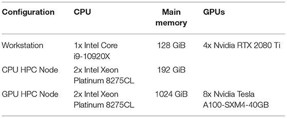
Table 1. Benchmark test hardware configurations.

TABLE 2

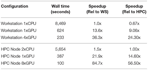
Table 2. Benchmark timing tests results.

3.3. Accuracy of the Results

The accuracy of the test results was assessed by using the MCMC chain samples to calculate prediction intervals for the number of reported daily incident cases. We then compared the coverage of the actual reported data against those prediction intervals. Doing this comparison for days in the projection time range, that is at times t > t_e,n, would introduce errors caused by the β(t) extrapolation method used in addition to any errors in the MCMC analysis itself. In order to isolate the MCMC analysis errors, we decided to calculate this coverage for days within the final windows time range t_b,n ≤ t ≤ t_e,n.

The reported number of cases on any given day, C_rep = C_true + ε_rep, is assumed to be the sum of the true number of cases C_true and some normally distributed reporting error ε_rep with 0 mean and variance of ${\sigma }_{rep}^2$. The MCMC process produces samples of the true number of cases C_true from the SEIR model output, and samples of the reporting error variance ${\sigma }_{rep}^2$ from the likelihood Equation (3). Under these assumptions, if we knew the exact value of σ_rep, then the probability density function f_Crep(x) = (f_Ctrue*Φ_0,σrep)(x) could be calculated as the convolution of f_Ctrue(x) with the normal probability density function Φ_0,σrep(x). However, because we do not know the exact value of σ_rep, we have to integrate over all possible values of σ_rep

$\begin{array}{ll}{f}_{C_{rep}}(x)={\displaystyle {\int }_0^{\infty }}\left[(f_{C_{true}}*{\Phi }_{0,{\sigma }_{rep}})(x)\right]f_{{\sigma }_{rep}}({\sigma }_{rep})d{\sigma }_{rep}& (4)\end{array}$

Due to the complexity of directly calculating (4), we chose instead to estimate the distribution by generating samples of C_rep from the samples of C_true and σ_rep that were stored while running Algorithm 1. To do so, we first randomly select a set {c_i ∈ C_true} from the set of true values and a set {σ_i ∈ σ_rep} from the set of reporting error variances. We can then draw samples of the reporting error $\left\{{\epsilon }_i~{N}(0,{\sigma }_i^2)\right\}$, let C_rep be the set {c_i + ε_i}, and estimate f_rep directly from those samples.

Prediction intervals were estimated from the samples by first applying a Box-Cox power transformation y_λ(C_rep) to the chain samples C_rep so that y_λ would be approximately normally distributed in the transformed domain [24]. From the normally distributed samples we could then calculate quantiles of interest from the inverse normal CDF ${\Phi }_{y_{\lambda }}^{-1}(p)$, and apply a reverse transform to get those points in the original domain. Those points were then used to estimate the prediction intervals PI(p) from the inverse CDF points as

$\begin{array}{ll}PI(p)=\left[y_{\lambda }^{-1}({\Phi }_{y_{\lambda }}^{-1}(.5-p/2)),y_{\lambda }^{-1}({\Phi }_{y_{\lambda }}^{-1}(.5+p/2))\right]& (5)\end{array}$

Each point in Figure 1 shows the prediction interval vs. coverage rate calculated on the set of 439 test jurisdictions. This value was calculated on the 29 different time windows and 50 prediction interval percentages for 1,450 points total.

FIGURE 1

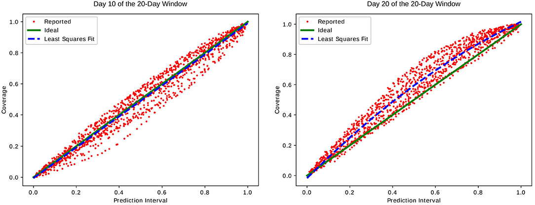
Figure 1. Prediction intervals of incident cases vs. coverage of reported data. Subfigures show this calculated on day 10 and day 20 of each 20-day window W_i. We can see that while we have good agreement on day 10 near the middle of each window, day 20 at the end of each window predicts too large of an interval resulting in a higher than expected coverage.

4. Discussion

We can see that although there is good agreement between the prediction interval and measured coverage for the middle of each window, the final day tends to over-predict the range. We hypothesize that the reason for this is at least in part that the likelihood Equation (3) does not take into account the autocorrelation of the residual ${\epsilon }^{(k)}=C^{(k)}-C_{true}^{(k)}$ from day to day. The real world reported case data does contain some time-dependent correlations in the reporting error. For instance, cases reported over the weekend tend to be lower than on weekdays when reporting staff are more likely to be working and processing the data. Similarly, Mondays and Tuesdays tend to report higher numbers as the backlog of cases not reported over the weekend is processed. On long enough time scales we expect this error to be nearly a stationary process, meaning that there should be almost no correlation in the values for days i ≠ j.

To illustrate the concept we ran the MCMC algorithm with the same loss Equation (3), but using a set of synthetically generated, time independent data, and also a simple linear model instead of an SEIR model. Figure 2 shows the timeseries plots of the samples selected from the MCMC algorithm along with the true values and reported data provided as input to the MCMC algorithm. The samples selected by the algorithm can be categorized as follows

1. The model output c_i begins much lower than the true value for days near the beginning of the window, crosses over the true value somewhere near the middle, and ends up much higher than the true value for days near the end

2. The model output c_i begins much higher than the true value for days near the beginning of the window, crosses over the true value somewhere near the middle, and ends up much lower than the true value for days near the end

3. Everything else

Because the samples from categories 1 and 2 overlap and both cross the true value near the middle of the window, the sample density closer to the middle of the window tends to be slightly higher than it is near the ends. Some preliminary testing of adding a Box Pierce Q test [25] term into the loss Equation (3) to test for the independence of the residual timeseries has shown to effectively reduce the severity of this over estimation in some synthetic test cases. At this time however, more research and testing would need to be done before any conclusions could be made about the correctness, general applicability, and effectiveness of such a method.

FIGURE 2

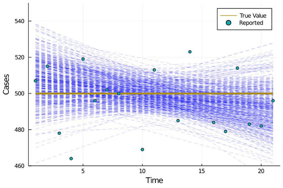
Figure 2. Synthetically generated test case illustrating why calculated confidence near the beginning and end of a window may tend to overpredict their range.

We presented a Multiple-Try Metropolis MCMC algorithm that can be parallelized and optimized to run on GPU and accelerate solving problems where the likelihood function involves running complex physics-based simulations. Examples of such problems include the original inspiration for our model, the plume reconstruction problem, the epidemiological model presented in this paper, problems from computational chemistry, and many more.

We presented as an example a simple SEIR model solved using IEM's BioSim simulator. The BioSim simulator itself features the capability to add additional compartments, aged transitions, and resource constraints to build a model that more closely matches real-world scenarios providing more accurate estimates of resource needs, such as hospital beds, ventilators, medication requirements, etc. Any of these features could be added to the underlying epidemiological model while maintaining the parallelization and acceleration provided by the GPUs.

In our testing, using a single GPU to execute the simulations resulted in more than a 13x speedup in wall clock time compared to a fully parallelized CPU implementation. The algorithm is also able to scale up to run on multiple GPUs. Using 4 Nvidia RTX 2080 Ti GPUs in a high-end developer's workstation resulted in a 36.3x speedup in wall clock time compared to running fully parallelized on the single Intel Core-i9-10920X CPU with 12 physical cores using 24 hyperthreads. The same tests on an AWS HPC server consisting of 8 Nvidia Tesla A100-SMX4-40GB GPUs resulted in a 56.5x speedup in wall clock time compared to running on the dual socket Intel Xeon Platinum 8275CL CPUs with a combined 48 physical cores and 96 hyperthreads.

Data Availability Statement

The raw data supporting the conclusions of this article will be made available by the authors, without undue reservation.

Author Contributions

BS developed the initial model idea and implemented the CPU and GPU optimized code to run the SEIR models and MCMC algorithm. BS and SS designed the main algorithms and developed the theoretical model formalism. PB supervised the project and provided oversight. All authors contributed to developing tests and analysis of the results and contributed to developing the manuscript and approved of its publication.

Conflict of Interest

BS, SS, HG, and PB are employed by IEM, Inc.

Publisher's Note

All claims expressed in this article are solely those of the authors and do not necessarily represent those of their affiliated organizations, or those of the publisher, the editors and the reviewers. Any product that may be evaluated in this article, or claim that may be made by its manufacturer, is not guaranteed or endorsed by the publisher.

References

1. Andrieu C, Freitas N, Doucet A, Jordan M. An introduction to MCMC for machine learning. Mach Learn. (2003) 50:5–43. doi: 10.1023/A:1020281327116

CrossRef Full Text | Google Scholar

2. Dunkley J, Bucher M, Ferreira PG, Moodley K, Skordis C. Fast and reliable markov chain monte carlo technique for cosmological parameter estimation. Mon Not R Astron Soc. (2005) 356:925–36. doi: 10.1111/j.1365-2966.2004.08464.x

CrossRef Full Text | Google Scholar

3. Valderrama-Bahamóndez GI, Fröhlich H. MCMC techniques for parameter estimation of ODE based models in systems biology. Front Appl Math Stat. (2019) 5:55. doi: 10.3389/fams.2019.00055

PubMed Abstract | CrossRef Full Text | Google Scholar

4. Craiu RV, Lemieux C. Acceleration of the multiple-try metropolis algorithm using antithetic and stratified sampling. Stat Comput. (2007) 17:109. doi: 10.1007/s11222-006-9009-4

CrossRef Full Text | Google Scholar

5. Robert CP, Elvira V, Tawn N, Wu C. Accelerating MCMC algorithms. Wiley Interdiscip Rev Comput Stat. (2018) 10:e1435. doi: 10.1002/wics.1435

PubMed Abstract | CrossRef Full Text | Google Scholar

6. Corander J, Gyllenberg M, Koski T. Bayesian model learning based on a parallel MCMC strategy. Stat Comput. (2006) 16:355–362. doi: 10.1007/s11222-006-9391-y

PubMed Abstract | CrossRef Full Text | Google Scholar

7. Martino L, Elvira V, Luengo D, Corander J, Louzada F. Orthogonal parallel MCMC methods for sampling and optimization. Digit Signal Process. (2016) 58:64–84. doi: 10.1016/j.dsp.2016.07.013

CrossRef Full Text | Google Scholar

8. Bédard M, Douc R, Moulines E. Scaling analysis of multiple-try MCMC methods. Stochastic Process Appl. (2012) 03;122:758–786. doi: 10.1016/j.spa.2011.11.004

CrossRef Full Text | Google Scholar

9. Cotter SL, Roberts GO, Stuart AM, White D. MCMC methods for functions: modifying old algorithms to make them faster. Stat Sci. (2013) 28:424–46. doi: 10.1214/13-STS421

CrossRef Full Text | Google Scholar

10. Girolami M, Calderhead B. Riemann manifold langevin and hamiltonian monte carlo methods. J R Stat Soc B. (2011) 73:123–214. doi: 10.1111/j.1467-9868.2010.00765.x

CrossRef Full Text | Google Scholar

11. Neal RM. MCMC Using Hamiltonian Dynamics. Boca Raton, FL: Chapman & Hall/CRC. (2012).

Google Scholar

12. Liu JS, Liang F, Wong WH. The multiple-try method and local optimization in metropolis sampling. J Am Stat Assoc. (2000) 95:121–34. doi: 10.1080/01621459.2000.10473908

CrossRef Full Text | Google Scholar

13. Bartz-Beielstein T, Stork J, Zaefferer M, Rebolledo M, Lasarczyk C, Rehbach F. CRAN SPOT plotSIRModel. Plot of Continuous Time Markov Chains SIR Models. (2020). Available online at: https://rdrr.io/cran/SPOT/man/plotSIRModel.html.

14. team B. SEIR 0.2.3. Python Package for Modeling Epidemics Using the SEIR Model. (2020). Availablable online at: https://pypi.org/project/SEIR/.

15. Mori JCM, Barbour W, Gui D, Piccoli B, Work D, Samaranayake S. A Multi-Region SEIR Model With Mobility. (2020). Available online at: https://seir.cee.cornell.edu/index.html.

16. Hall C, Ji W, Blaisten-Barojas E. The metropolis monte carlo method with CUDA enabled graphic processing units. J Comput Phys. (2014) 258:871–9. doi: 10.1016/j.jcp.2013.11.012

CrossRef Full Text | Google Scholar

17. Anderson RM, Anderson B, May RM. Infectious Diseases of Humans: Dynamics and Control. Oxford: Oxford University Press (1992).

Google Scholar

18. Li Q, Guan X, Wu P, Wang X, Zhou L, Tong Y, et al. Early transmission dynamics in wuhan, china, of novel coronavirus-infected pneumonia. N Engl J Med. (2020) 382:1199–207. doi: 10.1056/NEJMoa2001316

PubMed Abstract | CrossRef Full Text | Google Scholar

19. Martino L. A review of multiple try MCMC algorithms for signal processing. Digit Signal Process. (2018) 75:134–52. doi: 10.1016/j.dsp.2018.01.004

CrossRef Full Text | Google Scholar

20. Calderhead B. A general construction for parallelizing metropolis-hastings algorithms. Proc Natl Acad Sci USA. (2014) 111:17408–13. doi: 10.1073/pnas.1408184111

PubMed Abstract | CrossRef Full Text | Google Scholar

21. Ensheng Dong HD, Gardner L. An interactive web-based dashboard to track COVID-19 in real time. Lancet Infect Dis. (2020) 20:533–4. doi: 10.1016/S1473-3099(20)30120-1

PubMed Abstract | CrossRef Full Text | Google Scholar

22. Besard T, Foket C, De Sutter B. Effective extensible programming: unleashing julia on GPUs. IEEE Trans Parallel Distribut Syst. (2018) 30: 827–41. doi: 10.1109/TPDS.2018.2872064

CrossRef Full Text | Google Scholar

23. Besard T, Churavy V, Edelman A, De Sutter B. Rapid software prototyping for heterogeneous and distributed platforms. Adv Eng Softw. (2019) 132:29–46. doi: 10.1016/j.advengsoft.2019.02.002

CrossRef Full Text | Google Scholar

24. Box GEP, Cox DR. An analysis of transformations. J R Stat Soc B. (1964) 26:211–52. doi: 10.1111/j.2517-6161.1964.tb00553.x

CrossRef Full Text | Google Scholar

25. Box GEP, Pierce DA. Distribution of residual autocorrelations in autoregressive-integrated moving average time series models. J Am Stat Assoc. (1970) 65:1509–26. doi: 10.1080/01621459.1970.10481180

CrossRef Full Text | Google Scholar