Interpretable Transformed ANOVA Approximation on the Example of the Prevention of Forest Fires

The distribution of data points is a key component in machine learning. In most cases, one uses min-max-normalization to obtain nodes in [0, 1] or Z-score normalization for standard normal distributed data. In this paper, we apply transformation ideas in order to design a complete orthonormal system in the L₂ space of functions with the standard normal distribution as integration weight. Subsequently, we are able to apply the explainable ANOVA approximation for this basis and use Z-score transformed data in the method. We demonstrate the applicability of this procedure on the well-known forest fires dataset from the UCI machine learning repository. The attribute ranking obtained from the ANOVA approximation provides us with crucial information about which variables in the dataset are the most important for the detection of fires.

1. Introduction

In machine learning, the scale of our features is a key component in building models. When we work with data from applications, we have to accept it as it is. In most cases, we cannot control where the nodes are lying. Let us, e.g., take recommendations in online shopping. We are only able to analyze the customers that actually exist and what they bought in the shop. However, the features may lie on immensely different scales. If we measure, e.g., the time a customer spent in the shop in seconds, as well as their age in years, the result will be a scale that contains values with thousands of seconds and a scale ranging from up to 90 years. Bringing those features on similar scales trough normalization may significantly improve performance of our model.

Two common methods for data normalization are min-max-normalization and Z-score normalization, see, e.g.,[1]. The former method will yield data in the interval [0, 1] and is especially useful if there is an intrinsic upper and lower bound for the values, e.g., when considering age. If we come back to our previous example, the time a customer spends in the shop would be less suitable since the values may have a wide range and we will probably have very few people with a significantly small or large time. In this case, the Z-score normalization makes much more sense. It tells us how many standard deviations our value lies away from the mean of the data resulting in a distribution with zero mean and variance one.

The explainable ANOVA approximation method introduced in [2–4] is based on the well-known multi-variate analysis of variance (ANOVA) decomposition, see, e.g,.,[5–10], and relies on the existence of a complete orthonormal system in the space which is suitable for fast matrix-vector multiplication algorithms in grouped transformations, c.f.[11]. Until now, this method was always applied with min-max-normalization since it relied on the space ${\text{L}}_2({\left[0,1\right]}^d)$ of square-integrable functions over the cube with the half-period cosine basis. It is our goal to modify the approach in order to create the possibility to work with standard normal distributed data, i.e., data that has been obtained trough Z-score normalization.

We aim to achieve this by using the transformation ideas from [12] and [13] in order to construct a complete orthonormal system in the space

$\begin{array}{l}{\text{L}}_2({ℝ}^d,\omega )\text{ : =}\{f:{ℝ}^d\to ℝ:{\Vert f\Vert }_{{\text{L}}_2({ℝ}^d)}\\ \text{ : =}\sqrt{{\displaystyle {\int }_{{ℝ}^d}{\left|f(x)\right|}^2}\omega (x)dx}<\infty \}& (1)\end{array}$

with the probability density of the standard normal distribution

$\begin{array}{ll}\omega (x):\; ={\displaystyle \prod _{i=1}^d}\frac{1}{\sqrt{2\pi }}{\text{e}}^{-x_i^2/2}={(2\pi )}^{-d/2}{\text{e}}^{-\Vert x|{|}_2^2/2}.& (2)\end{array}$

The cumulative distribution function of the standard normal distribution is given by

$\begin{array}{ll}\Phi :ℝ\to \left[0,1\right],\Phi (x)=\frac{1}{2}\left[1+\text{erf}\left(\frac{x}{\sqrt{2}}\right)\right],& (3)\end{array}$

(see Figure 1) for visualization, with the error function defined as

$\begin{array}{l}\text{erf}(x)=\frac{2}{\sqrt{\pi }}{\displaystyle {\int }_0^x}{\text{e}}^{-t^2}\text{d}t.\end{array}$

Combining this transformation with the half-period cosine basis allows for fast multiplications in the grouped transformations and makes the ANOVA approximation method applicable for Z-score normalized data.

FIGURE 1

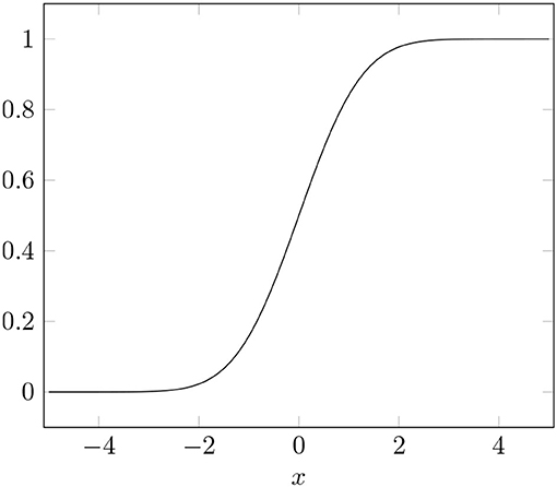
Figure 1. Cumulative distribution function Φ of the standard normal distribution from Equation (3).

As an example, we apply this approach to a dataset about the detection of forest fires, see [14, 15]. Constructing a model with the capability of efficiently predicting the size of the fire in this dataset may provide a way of predicting the occurrences of fires. This creates the possibility of efficiently implementing appropriate counter-measures. In our time of climate change with massive forest fires every year, e.g., in Australia or the USA, this is an extremely current topic. With the interpretation capabilities of the ANOVA method, c.f.[4], we are additionally able to explain the importance of our features and give reasonable explanation for the predictions.

2. Transformed Half-Period Cosine

In this section, it is our goal to construct a complete orthonormal system in the space ${\text{L}}_2({ℝ}^d,\omega )$ from Equation (1) with the product density ω(x) from Equation (2). This is the probability density function of the standard normal distribution, i.e., the normal distribution with zero mean and variance one. We have ${\int }_{{ℝ}^d}\omega (x)\text{d}x=1$, as well as ${sup}_{x\in {ℝ}^d}\omega (x)={(2\pi )}^{-d/2}$ which implies $\omega \in {\text{L}}_{\infty }({ℝ}^d)$.

We aim to construct the basis using transformation ideas from [12, 13] and the half-period cosine basis on ${\text{L}}_2({\left[0,1\right]}^d)$. The orthonormal basis functions on ${\text{L}}_2({\left[0,1\right]}^d)$ are given by

$\begin{array}{ll}{\varphi }_k^{\text{cos}}(x)={\sqrt{2}}^{\Vert k|{|}_0}{\displaystyle \prod _{i=1}^d}cos(\pi k_i{x}_i),k\in {\mathbb{N}}_0^d& (4)\end{array}$

with ‖k‖₀ := |supp k| for supp k := {s ∈ {1, 2, …, d}:k_s ≠ 0} and |supp k| the cardinality of supp k. We start from a given function f : ℝ^d → ℝ, $f\in {\text{L}}_2({ℝ}^d,\omega )$, and aim to transform it onto the cube [0, 1]^d. As transformation from the interval [0, 1] to ℝ, we apply the inverse cumulative distribution function Φ⁻¹ in each variable to obtain

$\begin{array}{ll}\psi :{\left[0,1\right]}^d\to {ℝ}^d,\psi (x)=\left(\begin{array}{c}{\Phi }^{-1}(x_1)\\ {\Phi }^{-1}(x_2)\\ ⋮\\ {\Phi }^{-1}(x_d)\end{array}\right)& (5)\end{array}$

with the inverse transformation being

$\begin{array}{ll}{\psi }^{-1}:{ℝ}^d\to {\left[0,1\right]}^d,{\psi }^{-1}(x)=\left(\begin{array}{c}\Phi (x_1)\\ \Phi (x_2)\\ ⋮\\ \Phi (x_d)\end{array}\right).& (6)\end{array}$

The transformation is related to inverse transform sampling, see, e.g.,[16]. As a result, we have the commutative diagram in Figure 2. This allows us to transform the half-period cosine to a complete orthonormal system on ${\text{L}}_2({ℝ}^d,\omega )$ with the help of the following lemma.

FIGURE 2

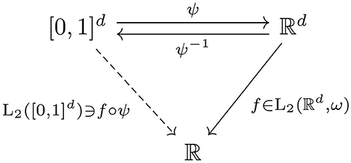
Figure 2. Commutative diagram of the function and the transformations.

Lemma 2.1. Let $g,h\in {\text{L}}_2({\left[0,1\right]}^d)$, $u,v\in {\text{L}}_2({ℝ}^d,\omega )$ with probability density ω from Equation (2), and transformation ψ, ψ⁻¹ as in Equations (5) and (6), respectively. Then

$\begin{array}{l}{\langle g\circ {\psi }^{-1},h\circ {\psi }^{-1}\rangle }_{{\text{L}}_2({ℝ}^d,\omega )}={\langle g,h\rangle }_{{\text{L}}_2({\left[0,1\right]}^d)}\\ {\langle u,v\rangle }_{{\text{L}}_2({ℝ}^d,\omega )}={\langle u\circ \psi ,v\circ \psi \rangle }_{{\text{L}}_2({\left[0,1\right]}^d)}\end{array}$

and subsequently $\Vert h{\Vert }_{{\text{L}}_2({\left[0,1\right]}^d)}=\Vert h\circ {\psi }^{-1}{\Vert }_{{\text{L}}_2({ℝ}^d,\omega )}$ and $\Vert u\circ \psi {\Vert }_{{\text{L}}_2({\left[0,1\right]}^d)}=\Vert u{\Vert }_{{\text{L}}_2({ℝ}^d,\omega )}$.

Proof. Let $g,h\in {\text{L}}_2({\left[0,1\right]}^d)$ and $u,v\in {\text{L}}_2({ℝ}^d,\omega )$. Then we insert the definition and perform a change of variables as follows

$\begin{array}{l}{\langle g\circ {\psi }^{-1},h\circ {\psi }^{-1}\rangle }_{{\text{L}}_2({ℝ}^d,\omega )}\\ ={\displaystyle {\int }_{{ℝ}^d}}g({\psi }^{-1}(x))h({\psi }^{-1}(x))\omega (x)\text{ d}x\\ ={\displaystyle {\int }_{{\left[0,1\right]}^d}}g(t)h(t)\omega (\psi (t))|det{\psi }^{\prime }(t)|\text{d}t.\end{array}$

As functional determinant we obtain $|det{\psi }^{\prime }(t)|={\prod }_{i=1}^d\sqrt{2\pi }{\text{e}}^{\text{er}{\text{f}}^{-2}(2t_i-1)}$ and subsequently

$\begin{array}{l}\omega (\psi (t))|det{\psi }^{\prime }(t)|={\displaystyle \prod _{i=1}^d}\frac{1}{\sqrt{2\pi }}{\text{e}}^{-\text{er}{\text{f}}^{-2}(2t_i-1)}·\sqrt{2\pi }{\text{e}}^{\text{er}{\text{f}}^{-2}(2t_i-1)}\\ =1.\end{array}$

This proves the first equality. For the second equality, we use an analogous procedure.

Lemma 2.1 is not surprising since we have based the transformation on the cumulative distribution function Φ from Equation (3). In the following, we obtain the new orthonormal system.

Theorem 2.2. The functions ${({\varphi }_k^{\text{trafo}})}_{k\in {\mathbb{N}}_0^d}$ with

$\begin{array}{ll}{\varphi }_k^{\text{trafo}}(x):\; =({\varphi }_k^{\text{cos}}\circ {\psi }^{-1})(x)={\sqrt{2}}^{\Vert k|{|}_0}{\displaystyle \prod _{i=1}^d}cos(\pi k_i\Phi (x_i))& (7)\end{array}$

form a complete orthonormal system in ${\text{L}}_2({ℝ}^d,\omega )$.

Proof. We have that Φ from Equation (3) is a bijection and Lemma 2.1 shows that f↦f ∘ ψ ⁻¹ is an isometric isomorphism between ${\text{L}}_2({ℝ}^d,\omega )$ and ${\text{L}}_2({\left[0,1\right]}^d)$. Now, an isometric isomorphism between two spaces maps an orthonormal basis in one space to an orthonormal basis in the other. We obtain that ${({\varphi }_k^{\text{trafo}})}_{k\in {\mathbb{N}}_0^d}$ is an orthonormal basis in ${\text{L}}_2({\left[0,1\right]}^d)$.

In summary, we have constructed a complete orthonormal system ${({\varphi }_k^{\text{trafo}})}_{k\in {\mathbb{N}}_0^d}$ on the weighted space ${\text{L}}_2({ℝ}^d,\omega )$ using transformation ideas from [13] and the well-known half-period cosine basis ${({\varphi }_k^{\text{cos}})}_{k\in {\mathbb{N}}_0^d}$ on ${\text{L}}_2({\left[0,1\right]}^d)$. The basis functions are visualized in Figure 3.

FIGURE 3

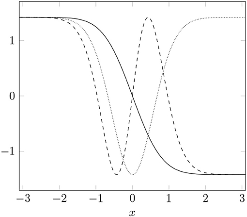
Figure 3. Transformed basis functions ${\varphi }_k^{\text{trafo}}$ for k = 1 (solid), k = 2 (dotted), and k = 3 (dashed), in one dimension.

3. Interpretable ANOVA Approximation

In this section, we briefly summarize the interpretable ANOVA (analysis of variance) approximation method and the idea of grouped transformations, see [2, 11]. The approach was considered for periodic functions, but has been expanded to non-periodic functions in [3, 4]. In this paper, we focus on functions f : ℝ^d → ℝ from ${\text{L}}_2({ℝ}^d,\omega )$ with probability density ω from Equation (2). Since ω is the density of the standard normal distribution, this function space is of a high relevance. It allows us, e.g., to work with data from applications that has been Z-transformed, i.e., data with zero mean and variance one, see, e.g.,[1]. Since the transformed half-period cosine ${({\varphi }_k^{\text{trafo}})}_{k\in {\mathbb{N}}_0^d}$, see Theorem 2.2, is a complete orthonormal system in the space ${\text{L}}_2({ℝ}^d,\omega )$, we have

$\begin{array}{ll}f(x)={\displaystyle \sum _{k\in {\mathbb{Z}}^d}}{\text{c}}_k(f){\varphi }_k^{\text{trafo}}(x),{\text{c}}_k(f)={\langle f,{\varphi }_k^{\text{trafo}}\rangle }_{{\text{L}}_2({ℝ}^d,\omega )},& (8)\end{array}$

and through Parseval's identity $\Vert f|{|}_{{\text{L}}_2({ℝ}^d,\omega )}^2=\sum _{k\in {\mathbb{Z}}^d}|{\text{c}}_k(f){|}^2$.

The classical ANOVA decomposition, c.f. [5–7, 9], provides us with a unique decomposition in the frequency domain as shown in [2]. We denote the set of coordinate indices with [d] = {1, 2, …, d}. The ANOVA terms are defined as

$\begin{array}{l}{f}_u(x)=f_u(x_u):\; ={\displaystyle \sum _{\begin{array}{c}k\in {\mathbb{Z}}^d\\ \text{supp}k=u\end{array}}}{\text{c}}_k(f){\varphi }_k^{\text{trafo}}(x).\end{array}$

The function can then be uniquely decomposed as

$\begin{array}{l}f(x)={\displaystyle \sum _{u\underset{\_}{\subset }\left[d\right]}{f}_u}(x)\end{array}$

into $|{P}(\left[d\right])|=2^d$ ANOVA terms where ${P}(\left[d\right])$ is the power set of [d]. Here, the exponentially growing number of terms shows an expression of the curse of dimensionality in the decomposition.

It is our goal to obtain information on how important the ANOVA terms f_u are with respect to the function f. In order to measure this, we define the variance of a function f as

$\begin{array}{l}{\sigma }^2(f):\; =\Vert f{\Vert }_{{\text{L}}_2({ℝ}^d,\omega )}^2-|{\text{c}}_0(f){|}^2={\displaystyle \sum _{k\in {\mathbb{Z}}^d\backslash \left\{0\right\}}}|{\text{c}}_k(f){|}^2.\end{array}$

Note that, we have the special case ${\sigma }^2(f_u)=\Vert f_u|{|}_{{\text{L}}_2({ℝ}^d,\omega )}^2$, u ⊆ [d]. The relative importance with respect to f is then measured via global sensitivity indices (GSI) or Sobol indices, see [7, 17, 18], defined as

$\begin{array}{ll}\varrho (u,f):\; =\frac{{\sigma }^2(f_u)}{{\sigma }^2(f)}.& (9)\end{array}$

From the GSI we get a motivation for the concept of effective dimensions, specifically the superposition dimension as one notion of effective dimension. For a given α ∈ [0, 1] it is defined as

$\begin{array}{ll}{\text{d}}^{(\text{sp})}:\; =min\left\{s\in \left[d\right]:\frac{1}{{\sigma }^2(f)}{\displaystyle \sum _{\begin{array}{c}u\subseteq \left[d\right]\\ |u|\le s\end{array}}}{\sigma }^2(f_u)\ge \alpha \right\}.& (10)\end{array}$

The superposition dimension d^(sp) tells us that we can explain the α-part of the variance of f by terms f_u with u ≤ d^(sp).

Using subsets of ANOVA terms $U\subseteq {P}(\left[d\right])$, it is our goal to find a way to circumvent the curse of dimensionality for efficient approximation. In order to achieve this, we aim to truncate the ANOVA decomposition by taking only the ANOVA terms in U into account. The truncated ANOVA decomposition is then defined as

$\begin{array}{l}{\text{T}}_{U}f(x)={\displaystyle \sum _{u\in U}}{f}_u(x).\end{array}$

A specific idea for the truncation comes from the superposition dimension d^(sp) in Equation (10). The idea is to take only variable interactions into account that contain d_s or less variables, i.e., the subset of ANOVA terms is

$\begin{array}{ll}U(d,d_s):\; =\left\{u\subseteq \left[d\right]:|u|\le d_s\right\}.& (11)\end{array}$

Here, we call d_s a superposition threshold. Since d_s does not necessarily have to coincide to the superposition dimension d^(sp), we call it superposition threshold. A well-known fact from learning theory is that the number of terms in U(d, d_s) grows only polynomially in d for fixed d_s < d, i.e.,

$|U(d,d_s)|\le {\left(\frac{\text{e}d}{d_s}\right)}^{d_s}$

which has reduced the curse of dimensionality.

In the following, we argue why the truncation by a superposition threshold d_s works well in relevant cases. For the approximation of functions that belong to a space $H^s({ℝ}^d,\omega )\subseteq {\text{L}}_2({ℝ}^d,\omega )$ that characterizes the smoothness s>0 by the decay of the basis coefficients c_k(f), we can show upper bounds on the superposition dimension d^(sp) for α ∈ [0, 1], see, e.g.,[2]. In fact, there are types of smoothness that are proven to yield a low upper bound for the superposition dimension specifically dominating-mixed smoothness with POD (product and order-dependent) weights, c.f. [2, 19–22].

In terms of real data from applications, the situation is much different. Here, we cannot make the assumption that in complete generality we have a low superposition dimension. However, there are many application scenarios where numerical experiments successfully showed that this is indeed the case, see, e.g., [5]. Since we generally do not have a-priori information, we work with low superposition thresholds d_s for truncation and validate on our test data.

3.1. Approximation Procedure

In this section, we briefly discuss how the approximation is numerically obtained and how we can interpreted the results. In this section, we assume a given subset of ANOVA terms $U\subseteq {P}(\left[d\right])$. This set may be equal to or a subset of U(d, d_s). We have given scattered data in the form of a set ${X}=\left\{x_1,x_2,\dots ,x_M\right\}\subseteq {ℝ}^d$ of standard normal distributed nodes and values y ∈ ℝ^M, M ∈ ℕ. Moreover, we assume that there is an ${\text{L}}_2({ℝ}^d,\omega )$ function f of form Equation (8) with f(x_i) ≈ y_i which we want to approximate.

First, we truncate f to the set U such that f ≈ T_Uf. However, there are still infinitely many coefficients and, therefore, we perform a truncation to partial sums on finite support index sets

$\begin{array}{ll}{{I}}_{\varnothing }=\left\{0\right\},\text{and}{{I}}_u={\{1,2,\dots ,N_{\left|u\right|}-1\}}^{\left|u\right|}& (12)\end{array}$

with order-dependent parameters N_|u| ∈ ℕ, |u| = 1, 2, …, d_s, for every ANOVA term f_u, u ∈ U. Using the projections $P_u{{I}}_u=\left\{k\in {\mathbb{N}}_0^d:k_u\in {{I}}_u,k_{u^c}=0\right\}$ with u^c: = [d]\u, we obtain

$\begin{array}{l}{f}_u(x)\approx {\displaystyle \sum _{k\in P_u{{I}}_u}}{\text{c}}_k(f){\varphi }_k^{\text{trafo}}(x).\end{array}$

Now, taking the union ${I}(U)={\bigcup }_{u\in U}{P}_u{{I}}_u$ yields

$f(x)\approx {\displaystyle \sum _{k\in {I}(U)}}{\text{c}}_k(f){\varphi }_k^{\text{trafo}}(x).$

However, the coefficients c_k(f) are unknown and it is our goal to determine approximations to them. We aim to achieve this by solving the regularized least-squares problem

$\begin{array}{ll}\widehat{f}={({\widehat{f}}_k)}_{k\in {I}(U)}=\underset{\widehat{g}\in {ℝ}^{\left|{I}(U)\right|}}{\text{arg min}}\Vert y-F({X},{I}(U))\widehat{g}{\Vert }_2^2+\lambda \Vert \widehat{g}{\Vert }_2^2,& (13)\end{array}$

c.f. [2, 3, 11], with the basis matrix $F({X},{I}(U))={({\varphi }_k^{\text{trafo}}(x))}_{x\in {X},k\in {I}(U)}$. For the approximate coefficients, we have ${\widehat{f}}_k\approx {\text{c}}_k(f)$ and we define the resulting approximation as

$\begin{array}{l}S({X},{I}(U))f:\; ={\displaystyle \sum _{k\in {I}(U)}}{\widehat{f}}_k{\varphi }_k^{\text{trafo}}.\end{array}$

We solve problem Equation (13) using the iterative LSQR solver [23]. In order to apply LSQR, we rewrite Equation (13) by observing the equality

$\begin{array}{ll}||y-F({X},{I}(U))\widehat{g}{||}_2^2+\lambda ||\widehat{g}{||}_2^2=\left|\right|\left(\begin{array}{c}y\\ 0\end{array}\right)-\left(\begin{array}{c}F\left({X},{I}\left(U\right)\right)\\ \sqrt{\lambda }I\end{array}\right)\widehat{g}|{|}_2^2& (14)\end{array}$

with 0 the zero vector in ${ℝ}^{\left|{I}(U)\right|}$ and I ∈ ℝ^{|I(U)|, |I(U)|} the identity matrix. Note that, we always have a unique solution in this case since the matrix

$\left(\begin{array}{c}F\left({X},{I}\left(U\right)\right)\\ \sqrt{\lambda }I\end{array}\right)$

has full column rank. However, the solution depends on the regularization parameter λ.

We apply the matrix-free variant of LSQR, i.e., we never explicitly construct the matrix $F({X},{I}(U))$. The grouped transformations introduced in [11] provide oracle functions for the multiplications of $F({X},{I}(U))$ and its transposed $F^{\mathrm{\text{T}}}({X},{I}(U))$ with vectors. For our specific basis functions ${\varphi }_k^{\text{trafo}}$ the grouped transformations are based on the non-equispaced fast cosine transform or NFCT, see [24, 25]. The transformation uses parallelization to separate our multiplication into smaller, up to d_s-dimensional NFCTs which results in an efficient algorithm. For more details we refer to [11].

One key fact is that the nodes ${X}$ have to be distributed according to the probability density ω of the space such that the Moore–Penrose inverse $F^{†}({X},{I}(U))$ is well-conditioned. In our case, ω is the density of the standard normal distribution, i.e., the nodes ${X}$ have to be distributed accordingly. For a detailed discussion on the properties of those matrices we refer to [26, 27] where our basis is a special case.

We use the global sensitivity indices $\varrho (u,S({X},{I}(U))f)$, u∈U, from the approximation $S({X},{I}(U))f(x)$ to compute approximations for the global sensitivity indices ϱ(u, f) of the function f. Here, we do not consider the index to be a good approximation if the values are close together, but rather if there order is identical, i.e., we have

$\begin{array}{l}\varrho (u_1,f)\le \varrho (u_2,f)\Rightarrow \varrho (u_1,S({X},{I}(U))f)\le \varrho (u_2,S({X},{I}(U))f)\end{array}$

for any pair u₁, u₂ ∈ U. We assume that this is the case for our choices of index sets ${I}(U)$. In particular, the quality of the approximation corresponds to the accuracy of this assumption.

In order to rank the influence of the variables x₁, x₂, …, x_d we use the ranking score

$\begin{array}{rr}r\left(i\right)=\frac{\begin{array}{r}{\sum }_{u\in \left\{v\in U:i\in v\right\}}|\left\{v\in U:|u|=|v|,i\in v\right\}{|}^{-1}\\ \varrho \left(u,S\left({X},{I}\left(U\right)\right)f\right)\end{array}}{\begin{array}{r}{\sum }_{u\in U}\left({\sum }_{j\in u}|\left\{v\in U:|u|=|v|,j\in v\right\}{|}^{-1}\right)\\ \varrho \left(u,S\left({X},{I}\left(U\right)\right)f\right)\end{array}}.& (15)\end{array}$

for i = 1, 2, …, d which was introduced in [4]. Note that this score has order-dependent weight and is normalized such that $\sum _{i\in \left[d\right]}r(i)=1$. Computing every score r(i), i ∈ [d] provides an attribute ranking with respect to U showing the percentage that every variable adds to the variance of the approximation. We then conclude that if we have a good approximation $S({X},{I}(U))f$, the corresponding attribute ranking will be close to the attribute ranking of the function f.

3.2. Active Set

In this section, we describe how to obtain a set of ANOVA terms U for approximation. We are still working with the scattered data ${X}\subseteq {ℝ}^d$ and y ∈ ℝ^M, M ∈ ℕ. The values y may also contain noise. Our first step is to limit the variable interactions by a superposition threshold d_s ∈ [d] which may have been estimated by known smoothness properties (or different a-priori information) or set to a sensible value if nothing is known. It is also possible to determine an optimal value through cross-validation. We choose the order-dependent parameters N_|u|, |u| = 1, 2, …, d_s, c.f. Equation (12), to obtain ${I}(U(d,d_s))$ and with the procedure described in Section 3.1, the approximation $S({X},{I}(U(d,d_s)))f$.

From the approximation $S({X},{I}(U(d,d_s)))f$ we can then calculate the global sensitivity indices $\varrho (u,S({X},{I}(U(d,d_s)))f)$, u ∈ U(d, d_s), and an attribute ranking r(i), i ∈ [d], see Equation (15). Then we are able to apply the strategies proposed in [4] to truncate terms from the set U(d, d_s).

One obvious method is the truncation of an entire variable x_i, i ∈ [d], if the attribute ranking r(i) shows that its influence is insignificant. Specifically, that would translate to an active set $U^{*}=\left\{u\in U(d,d_s):\text{i}\notin u\right\}$. This leads to a reduction in dimensionality of the problem and greatly simplifies our model.

A different method is active set thresholding where we chooses a threshold vector $\text{ε}\in {(0,1)}^{d_s}$ and reduce the ANOVA terms to the set

$\begin{array}{l}{U}^{*}(\text{ε}):\; =\left\{u\in U(d,d_s):\varrho (u,S({X},{I}(U(d,d_s)))f)>{\text{ε}}_{\left|u\right|}\right\}.\end{array}$

Here, ε_|u| denotes the |u|th entry of the vector ε. The parameter vector ε allows control over how much of the variance may be sacrificed in order to simplify the model function.

In summary, it is necessary to interpret the information from the approximation $S({X},{I}(U(d,d_s)))f$ and decide on strategies for truncating the set of ANOVA terms. One may also use different strategies to obtain an active set or any combination of the multiple approaches, see, e.g.,[3, 4]. Of course, it is also possible to repeat the procedure multiple times, i.e., through cross-validation.

4. Forest Fire Prevention

We now apply the previously described method to the dataset [14] from the UC Irvine machine learning repository. The dataset contains information about forest fires in the Montesinho national park in the Trás-os-Montes northeast region of Portugal. The data was collect from 2002 to 2003. Specifically, we have d = 12 attributes about the fires and the target variable is the area of the forest that was destroyed by it. If we obtain an efficient model, it can be possible to predict the risk for a future forest fire using parameters that can be easily measured. This information can then be used to prepare appropriate countermeasures. The dataset has been thoroughly considered in [15] and we compare to the results they obtained. The authors considered several different methods: the naive average predictor (Naive), multiple regression (MR), decision tree (DT), random forest (RF), neural network (NN), and support vector machine (SVM).

We group the 12 attributes into 4 categories as in [15], i.e., spatial, temporal, FWI system, and meteorological data, (see Table 1). The spatial attributes describe the spatial location of the fire in a 9 by 9 grid of our considered region. The temporal attributes are the month of the year and the day of the week when the fire occurred. The forest fire weather index (FWI), c.f.[28], is the Canadian system for rating fire danger and the dataset collects several components of it, see also Table 2. Moreover, four meteorological attributes which are used by the FWI index were selected. The target variable describes the area that was burned by the fire.

TABLE 1

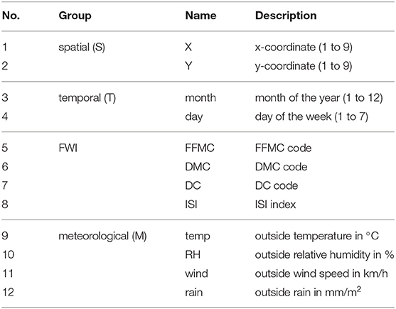
Table 1. Attributes of the forest fires dataset and their corresponding groups.

TABLE 2

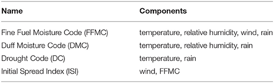
Table 2. Codes of the FWI with their base components from the weather data according to [28].

In terms of pre-processing, we apply a Z-score transformation to the variables and the logarithmic transformation log(1+·) to the burned area. The Z-score transformation achieves that our data has zero mean and unit variance. The logarithmic transformation on the target is opportune since it shows a positive skew with a large number of fires that have a small size. We denote the data $({X},y)$ with ${X}=\left\{x_1,x_2,\dots ,x_M\right\}\subseteq {ℝ}^{12}$, M = 517, and y ∈ ℝ^M. In the following, we do not use all of the variables, but build models based only on some groups as denoted in Table 1, e.g., STM says that we use spatial, temporal, and meteorological attributes without the FWI.

Table 3 shows the overall results of our experiment (ANOVA) combined with the benchmark data from [15]. Each value, our ANOVA results, as well as the others, were obtained by averaging over executing a 10-fold cross-validation 30 times. This results in a total of 300 experiments. We used a superposition threshold of d_s = 2, c.f. Equation (11), and, therefore, needed to detect optimal choices for the parameters N₁ and N₂ from Equation (12), (see Table 4). Every experiment utilized 90% of the data as training set $({{X}}_{\text{train}},y_{\text{train}})$ and 10% of the data as test set $({{X}}_{\text{test}},y_{\text{test}})$. The best performing model was selected based on the mean absolute deviation

$\begin{array}{ll}\text{MAD}=\frac{1}{\left|{{X}}_{\text{test}}\right|}{\displaystyle \sum _{i=1}^{\left|{{X}}_{\text{test}}\right|}}|{(\tilde{y})}_i-{(y_{\text{test}})}_i|& (16)\end{array}$

with $\tilde{y}$ the predictions of our model for the data points in the test set ${{X}}_{\text{test}}$. As a second error measure, we use the root mean square error.

$\begin{array}{ll}\text{RMSE}=\frac{1}{\sqrt{\left|{{X}}_{\text{test}}\right|}}\sqrt{{\displaystyle \sum _{i=1}^{\left|{{X}}_{\text{test}}\right|}}|{(\tilde{y})}_i-{(y_{\text{test}})}_i{|}^2}.& (17)\end{array}$

We are able to outperform the previously applied method for every subset of attributes in both MAD and RMSE error. Notably, the difference in the RMSE that penalizes larger deviations in the burned area stronger than the MAD is much more significant.

TABLE 3

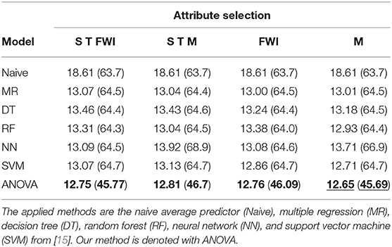
Table 3. MAD and RMSE (in brackets) for the best performing model in the corresponding attribute subset (underline—overall best result, bold—best result for this selection).

TABLE 4

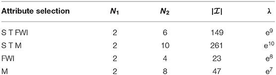
Table 4. Optimal parameter choices for the experiments from Table 3.

While we replicated the setting of [15] for benchmark purposes, it remains our goal to identify the most important attributes for the detection of forest fires. Therefore, we now use all 12 attributes of the dataset in obtaining our approximation and subsequently interpret the results. Figure 4 shows the attribute ranking r(i), i = 1, 2, …, 12, and Figure 5 the global sensitivity indices $\varrho (u,S({{X}}_{\text{train}},{I}(U(12,2)))f)$, u ∈ U(12, 2), after computing for an approximation with N₁ = N₂ = 2 and λ = 1.0.

FIGURE 4

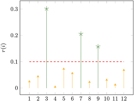
Figure 4. Attribute ranking r(i), i = 1, 2, …, 12, of the approximation with all twelve attributes using N₁ = N₂ = 2 and λ = 1.0.

FIGURE 5

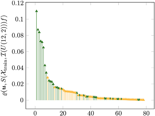
Figure 5. Global sensitivity indices $\varrho (u,S({{X}}_{\text{train}},{I}(U(12,2)))f)$, $u\in {I}(U(12,2))$, of the approximation with all twelve attributes using N₁ = N₂ = 2 and λ = 1.0 (sorted). The green indices belong to sets u such that ∃s ∈ {3, 7, 9} with s ∈ u.

The attributes 3, 7, and 9 are clearly the most important. They represent the month of the year (3), the DC code of the FWI (7), and the outside temperature (9). Using only these three attributes and superposition threshold d_s = 2, we computed an approximation with N₁ = 2, N₂ = 10, and λ = e⁸. The resulting model yielded an MAD of 12.64 and an RMSE of 45.57 with 30 times of 10-fold cross validation as before. In summary, we know that the most important information of our problem is contained in only three attributes and we also obtained a better performing model using only those three attributes.

Data Availability Statement

The original contributions presented in the study are included in the article/supplementary material, further inquiries can be directed to the corresponding author/s.

Author Contributions

Both authors listed have made a substantial, direct, and intellectual contribution to the work and approved it for publication.

Funding

DP acknowledges funding by Deutsche Forschungsgemeinschaft (German Research Foundation)—Project–ID 416228727—SFB 1410. MS was supported by the German Federal Ministry of Education and Research grant 01|S20053A. The publication of this article was funded by Chemnitz University of Technology.

Conflict of Interest

The authors declare that the research was conducted in the absence of any commercial or financial relationships that could be construed as a potential conflict of interest.

Publisher's Note

All claims expressed in this article are solely those of the authors and do not necessarily represent those of their affiliated organizations, or those of the publisher, the editors and the reviewers. Any product that may be evaluated in this article, or claim that may be made by its manufacturer, is not guaranteed or endorsed by the publisher.

Acknowledgments

The authors thank their colleagues in the research group SAlE for valuable discussions on the contents of this paper. Moreover, we thank the reviewers for their valuable comments and suggestions.

References

1. Hastie T, Tibshirani R, Friedman J. The Elements of Statistical Learning - Data Mining, Inference, and Prediction. New York, NY: Springer (2013).

PubMed Abstract | Google Scholar

2. Potts D, Schmischke M. Approximation of high-dimensional periodic functions with Fourier-based methods. SIAM J Numer Anal. (2021) 59:2393–429. doi: 10.1137/20M1354921

CrossRef Full Text | Google Scholar

3. Potts D, Schmischke M. Learning multivariate functions with low-dimensional structures using polynomial bases. J Comput Appl Math. (2022) 403:113821. doi: 10.1016/j.cam.2021.113821

CrossRef Full Text | Google Scholar

4. Potts D, Schmischke M. Interpretable approximation of high-dimensional data. SIAM J Math Data Sci. (2021) 3:1301–23. doi: 10.1137/21M1407707

CrossRef Full Text | Google Scholar

5. Caflisch R, Morokoff W, Owen A. Valuation of mortgage-backed securities using Brownian bridges to reduce effective dimension. J Comput Finance. (1997) 1:27–46.

Google Scholar

6. Rabitz H, F Alis O. General foundations of high dimensional model representations. J Math Chem. (1999) 25:197–233.

PubMed Abstract | Google Scholar

7. Liu R, Owen AB. Estimating mean dimensionality of analysis of variance decompositions. J Amer Statist Assoc. (2006) 101:712–21. doi: 10.1198/016214505000001410

CrossRef Full Text | Google Scholar

8. Kuo FY, Sloan IH, Wasilkowski GW, Woźniakowski H. On decompositions of multivariate functions. Math Comput. (2009) 79:953–66. doi: 10.1090/S0025-5718-09-02319-9

CrossRef Full Text | Google Scholar

9. Holtz M. “Sparse grid quadrature in high dimensions with applications in finance and insurance,” In: Lecture Notes in Computational Science and Engineering. Vol. 77. Berlin; Heidelberg: Springer (2011).

Google Scholar

10. Owen AB. Monte Carlo theory, methods and examples. (2013). Available online at: https://artowen.su.domains/mc/

Google Scholar

11. Bartel F, Potts D, Schmischke M. Grouped transformations in high-dimensional explainable ANOVA approximation. SIAM J Sci Comput. (2022). Available online at: https://arxiv.org/abs/2010.10199

Google Scholar

12. Nichols JA, Kuo FY. Fast CBC construction of randomly shifted lattice rules achieving ${O}(n^{-1+\delta })$ convergence for unbounded integrands over ℝ^s in weighted spaces with POD weights. J Complex. (2014) 30:444–68. doi: 10.1016/j.jco.2014.02.004

CrossRef Full Text | Google Scholar

13. Nasdala R, Potts D. Transformed rank-1 lattices for high-dimensional approximation. Electron Trans Numer Anal. (2020) 53:239–82. doi: 10.1553/etna_vol53s239

PubMed Abstract | CrossRef Full Text | Google Scholar

14. Forest Fires (2008). UCI Machine Learning Repository. Available online at: https://archive-beta.ics.uci.edu/ml/datasets/forest+fires

Google Scholar

15. Cortez P, Morais A. A data mining approach to predict forest fires using meteorological data. In: New Trends in Artificial Intelligence, 13th EPIA 2007 - Portuguese Conference on Artificial Intelligence. Guimarães: APPIA (2007). p. 512–23.

Google Scholar

16. Hörmann W. Automatic Nonuniform Random Variate Generation. Berlin: Springer (2004).

Google Scholar

17. Sobol IM. On sensitivity estimation for nonlinear mathematical models. Matem Mod. (1990) 2: 112–8.

Google Scholar

18. Sobol IM. Global sensitivity indices for nonlinear mathematical models and their Monte Carlo estimates. Math Comput Simulat. (2001) 55:271–280. doi: 10.1016/S0378-4754(00)00270-6

CrossRef Full Text | Google Scholar

19. Kuo FY, Schwab C, Sloan IH. Quasi-Monte Carlo finite element methods for a class of elliptic partial differential equations with random coefficients. SIAM J Numer Anal. (2012) 50:3351–74. doi: 10.1137/110845537

CrossRef Full Text | Google Scholar

20. Graham IG, Kuo FY, Nichols JA, Scheichl R, Schwab C, Sloan IH. Quasi-Monte Carlo finite element methods for elliptic PDEs with lognormal random coefficients. Numer Math. (2014) 131:329–68. doi: 10.1007/s00211-014-0689-y

CrossRef Full Text | Google Scholar

21. Kuo FY, Nuyens D. Application of Quasi-Monte Carlo methods to elliptic PDEs with random diffusion coefficients: a survey of analysis and implementation. Found Comput Math. (2016) 16:1631–96. doi: 10.1007/s10208-016-9329-5

CrossRef Full Text | Google Scholar

22. Graham IG, Kuo FY, Nuyens D, Scheichl R, Sloan IH. Circulant embedding with QMC: analysis for elliptic PDE with lognormal coefficients. Numer Math. (2018) 140:479–511. doi: 10.1007/s00211-018-0968-0

PubMed Abstract | CrossRef Full Text | Google Scholar

23. Paige CC, Saunders MA. LSQR: an algorithm for sparse linear equations and sparse least squares. ACM Trans Math Softw. (1982) 8:43–71.

Google Scholar

24. Keiner J, Kunis S, Potts D. Using NFFT3 - a software library for various nonequispaced fast Fourier transforms. ACM Trans Math Softw. (2009) 36:1–30. doi: 10.1145/1555386.1555388

CrossRef Full Text | Google Scholar

25. Plonka G, Potts D, Steidl G, Tasche M. Numerical Fourier Analysis. In: Applied and Numerical Harmonic Analysis. Cham: Birkhäuser (2018).

Google Scholar

26. Kämmerer L, Ullrich T, Volkmer T. Worst case recovery guarantees for least squares approximation using random samples. Constr Approx. (2021) 54:295–352. doi: 10.1007/s00365-021-09555-0

CrossRef Full Text | Google Scholar

27. Moeller M, Ullrich T. L₂-norm sampling discretization and recovery of functions from RKHS with finite trace. Sampl Theory Sign Process Data Anal. (2021) 19:13. doi: 10.1007/s43670-021-00013-3

CrossRef Full Text | Google Scholar

28. Taylor SW, Alexander ME. Science, technology, and human factors in fire danger rating: the Canadian experience. Int J Wildland Fire. (2006) 15:121. doi: 10.1071/WF05021

PubMed Abstract | CrossRef Full Text | Google Scholar