Bregman iterative regularization using model functions for nonconvex nonsmooth optimization

In this paper, we propose a new algorithm called ModelBI by blending the Bregman iterative regularization method and the model function technique for solving a class of nonconvex nonsmooth optimization problems. On one hand, we use the model function technique, which is essentially a first-order approximation to the objective function, to go beyond the traditional Lipschitz gradient continuity. On the other hand, we use the Bregman iterative regularization to generate solutions fitting certain structures. Theoretically, we show the global convergence of the proposed algorithm with the help of the Kurdyka-Łojasiewicz property. Finally, we consider two kinds of nonsmooth phase retrieval problems and propose an explicit iteration scheme. Numerical results verify the global convergence and illustrate the potential of our proposed algorithm.

1. Introduction

In this paper, we consider the following optimization problem

$\begin{array}{ll}{\displaystyle \underset{x\in {ℝ}^d}{min}}\psi (x):=f(x)+\mu R(x),& ({P})\end{array}$

where f, R : ℝ^d → (−∞, +∞] are given extended real-valued functions, and μ > 0 is some fixed parameter.

Bregman iterative regularization, originally proposed in Osher et al. [1] for total-variation-based image restoration, has become a popular technique for solving optimization problems with the form (${P}$). To simplify its computation, the linearized Bregman iterations (LBI) [2] and their variants [3–5] were proposed with lots of applications in signal/image processing and compressed sensing. Previous studies mainly focused on convex smooth optimization in the sense that both functions f and R in (${P}$) are convex and f is also smooth. Very recently, nonconvex smooth extensions of LBI were considered in Benning et al. [6] and later in Zhang et al. [7]. However, it seems unclear whether the LBI can be extended to nonconvex and nonsmooth cases. In other words, can we develop the LBI to solve (${P}$) with a nonconvex nonsmooth function f? This question is the main motivation of this study.

A basic algorithmic strategy for optimization problem (${P}$) is to successively minimize simple objective functions, usually called model functions, which approximate the original objective ψ near the current iterate. The LBI method is in the same spirit as this strategy; it uses a second-order Taylor expansion of f to approximate the smooth function f and uses a Bregman distance to replace the regularization function R. To deal with nonsmooth function f, however, it is impossible to use Taylor approximations. Fortunately, there recently developed several “Taylor-like” model functions techniques [8–10] to approximate and minimize a nonsmooth objective function f. In particular, the authors of Mukkamala et al. [10] introduced the concept of model approximation property (MAP) for extending the Bregman proximal gradient method to minimize a nonsmooth f.

In this paper, we will blend the techniques involved in LBI and MAP to propose a new iterative scheme for solving nonconvex and nonsmooth optimization problems (${P}$), along with completed convergence analysis. Moreover, we apply our proposed method to nonsmooth phase retrieval problems to demonstrate our findings, both theoretically and numerically.

The remainder of the paper is organized as follows. In Section 2, we introduce the Bregman distance, the concept of MAP, and also the Kurdyka-Łojasiewicz (KL) property. In Section 3, we propose our algorithmic scheme and a group of assumptions. In Section 4, we present a convergence analysis. The application demonstrations are given in Section 5 and Section 6. Finally, concluding remarks are discussed in Section 7.

2. Preliminaries

Throughout the paper, we work in a d-dimensional Euclidean vector space ℝ^d equipped with inner product 〈·, ·〉 and induced norm ||·||, where d ∈ ℕ\{0} (ℕ is the set of non-negative integers). The notation and almost all the facts about the convex analysis we employ are primarily taken from Rockafellar [11]. For a set B ⊂ ℝ^d, defined $||B|{|}_{-}:={inf}_{x\in B}||x||$. Let h be a convex function, dom h (h*, ∇h, ∂h) denotes the domain of h (conjugate function of h, gradient of h, and subgradient of h, respectively), and int dom h denote the interior domain of h. In addition, let ∂_xf(x; y) denote the subgradient of the function f(x; y) with respect to the first variable, ∂_yf(x; y) denote the subgradient of the function f(x; y) with respect to the second variable, and ∂f(x; y) denote the subgradient of f(x; y) with respect to (x, y).

2.1. Bregman distance

The concept of Bregman distance [12] is the most important technique in Bregman iterative regularization. Given a smooth convex function h, its Bregman distance between two points x and y is defined as

$\begin{array}{l}{D}_h(x,y):=h(x)-h(y)-\langle \nabla h(y),x-y\rangle .\end{array}$

Due to the convexity of h, it is essential that D_h is nonnegative but fails to hold the symmetry and the triangle inequality in general. The class of Legendre functions [13] provides a choice to generate Bregman distance.

Definition 2.1. (Legendre functions, Rockafellar [11]) Let h : ℝ^d → (−∞, +∞] be a proper lower semi-continuous (lsc) convex function. It is called:

• essentially smooth, if int dom h ≠ ∅, h is differentiable on int dom h, and ||∇h(x^k)|| → ∞ for every sequence ${\left\{x^k\right\}}_{k\ge 0}\subseteq \text{int dom }h$ converging to a boundary point of dom h as k → ∞;

• of Legendre type, if h is essentially smooth and strictly convex on int dom h.

As a special case of Legendre functions, the energy kernel $h=\frac{1}{2}||·|{|}^2$ yields the classical squared Euclidean distance.

Note that the common sparsity constraint R(·) = ||·||₁ is not of Legendre type since it is nonsmooth. It leads to the concept of generalized Bregman distance introduced by Kiwiel [14]. Given a proper lsc convex function R, the generalized Bregman distance associated with R between x, y with respect to a subgradient y* is defined by

$\begin{array}{l}{D}_R^{y^{*}}(x,y):=R(x)-R(y)-\langle y^{*},x-y\rangle ,\forall x\in \text{dom }R,y^{*}\in \text{dom }\partial R(y).\end{array}$

Properties of Bregman distances and examples of kernels can be referred to Kiwiel [14, 15], Chen and Teboulle [16], and Bauschke et al. [17].

2.2. Model function and model approximation property

Section 1 has briefly mentioned the model function and the MAP. Now we state its formal definition in Mukkamala et al. [10].

Definition 2.2. (Model function [10]) Let f be a proper lsc function. A function $f(·;\overline{x}):{ℝ}^d\to (-\infty ,+\infty ]$ with $\text{dom }f(·,\overline{x})=\text{dom }f$ is called a model function for f around the model center $\overline{x}\in dom f$, if there exists a growth function ${\varsigma }_{\overline{x}}:{ℝ}_{+}\to {ℝ}_{+}$ such that the following is satisfied:

$\begin{array}{l}|f(x)-f(x;\overline{x})|\le {\varsigma }_{\overline{x}}(||x-\overline{x}||),\forall x\in \text{dom }f.\end{array}$

The model function is essentially an approximation to f, and the growth function can be considered as a bound on the model error. Based on Definition 2.2, a modification of the model approximation property (MAP) (Definition 7, [10]) can be stated as below:

Definition 2.3 (Model approximation property). Let h be a Legendre function that is continuously differentiable over int dom h. A proper lsc function f with dom f ⊃ dom h and model function $f(·;\overline{x})$ for f around $\overline{x}\in \text{int dom }h$ satisfy the model approximation property at $\overline{x}$, with the constant L > 0, if for any $\overline{x}$ the following holds:

$\begin{array}{l}|f(x)-f(x;\overline{x})|\le L{D}_h(x;\overline{x}),\forall x\in \text{int dom }h.\end{array}$

2.3. Kurdyka-Łojasiewicz property

The Kurdyka-Łojasiewicz property is a significant tool for our global convergence analysis, which is defined as follows:

Definition 2.4. (Kurdyka-Łojasiewicz property and function [18]) The function F : ℝ^d → (−∞, +∞] is said to have the Kurdyka-Łojasiewicz property at x* ∈ dom(∂F) if there exists η ∈ (0, +∞], a neighborhood U of x* and a continuous concave function φ:[0, η) → ℝ₊ such that

(i) φ(0) = 0.

(ii) φ is C¹ on (0, η).

(iii) for all s ∈ (0, η), φ′(s) > 0.

(iv) for all x in U ∩ [F(x*) < F(x) < F(x*) + η], the Kurdyka-Łojasiewicz inequality holds

$\begin{array}{l}{\phi }^{\prime }(F(x)-F(x^{*}))\text{dist}(0,\partial F(x))\ge 1.\end{array}$

Additionally, a proper lsc function F that satisfies the Kurdyka-Łojasiewicz inequality at each point of dom(∂F) is called a KL function.

Usually, it may be difficult to verify the KL property of a function. Bolte et al. [19, 20] established a nonsmooth version of Kurdyka-Łojasiewicz inequality:

Lemma 2.5. Let F : ℝ^d → (−∞, +∞] be a proper lsc function. If F is semi-algebraic then it satisfies the KL property at any point of dom F.

Lemma 2.5 provides a result that KL property holds for the class of semi-algebraic functions. Semi-algebraic examples are common such as derivatives and ||·||_p. In addition, the class of semi-algebraic sets is stable under finite sums, compositions, or products [18].

3. Problem setting and ModelBI algorithm

Throughout this paper, we consider the optimization problem (${P}$) and make the following assumptions about the relative function h, the regularized function R, and the loss function f.

Assumption 3.1. (i) h : ℝ^d → (−∞, +∞] is of Legendre type and of ${{C}}^2$ over int dom h.

(ii) $R:{ℝ}^d\to {ℝ}_{+}$ is proper lsc convex with dom ∂R ⊃ int dom h and dom R ∩ int dom h ≠ ∅.

(iii) f:ℝ^d → (−∞, +∞] is proper lsc nonconvex nonsmooth with dom f ⊃ dom h and continuous on dom h. Moreover, the MAP holds for the pair of functions (f, h).

(iv) $-\infty <{inf}_{x\in \text{dom }h}f(x)$.

Assumption 3.2. Let p^k ∈ ∂R(x^k). If {x^k} ⊂ int dom h converges to some x ∈ dom h, then $D_h(x,x^k)\to 0$ and $D_R^{p^k}(x,x^k)\to 0$.

Assumption 3.3. For any bounded subset U ⊂ int dom h, there exists a constant L_h > 0 such that for any x ∈ U, h has bounded second derivative $||{\nabla }^{2}h(x)||\le L_h$.

Assumption 3.4. For any bounded set B ⊂ dom f, there exists c > 0 such that for any x, y ∈ B we have

$\begin{array}{l}||{\partial }_{y}f(x;y)|{|}_{-}\le c||x-y||.\end{array}$

Assumption 3.5. The regularized function R has locally bounded subgradients in the sense that if for any bounded set U ⊂ dom R there exists a constant C > 0 such that for any x ∈ U and all p ∈ ∂R(x) we have ||p|| ≤ C.

A few remarks about the assumptions are as follows:

• Assumptions 3.1(i) and (iii) are required by the MAP, among which $h\in {{C}}^2$ is needed for the surrogate function in Section 4. The assumptions of domains in (ii) ensure that the objective in Algorithm 1 is well-defined for x^k ∈ int dom h. (ii) can be satisfied if R is real-valued, for example, R(x) = ||x||₁. With respect to (iv), an lsc coercive function can ensure the compactness of its lower level set.

• A real-valued convex function R always holds that $D_R^{p^k}(x,x^k)\to 0$ as x^k → x due to the continuity of R [21, Theorem 3.16] and has locally bounded subgradients, which verifies Assumption 3.2 and Assumption 3.5.

• Assumption 3.4 governs the variation of the model function around the model center [10]. We can take the composite function f(G(x)) = |x² − 1| as a simple example. Its model function is $f(x;\overline{x})=f(G(\overline{x})+\langle \nabla G(\overline{x}),x-\overline{x}\rangle )=|{\overline{x}}^2-1+\langle 2\overline{x},x-\overline{x}\rangle |$. Then the subdifferential of the model function is given by ${\partial }_{y}f(x;\overline{x})=2\text{sgn}({\overline{x}}^2-1+\langle 2\overline{x},x-\overline{x}\rangle )(x-\overline{x})$, where sgn(x) = x/|x| if x ≠ 0 while sgn(0) ∈ [−1, 1]. Since |sgn(x)| ≤ 1, we have $|{\partial }_{y}f(x;\overline{x}){|}_{-}\le 2|x-\overline{x}|$.

Equipped with the above assumptions, the ModelBI algorithm for solving the nonconvex nonsmooth composite problem (${P}$) is described in Algorithm 1.

ALGORITHM 1

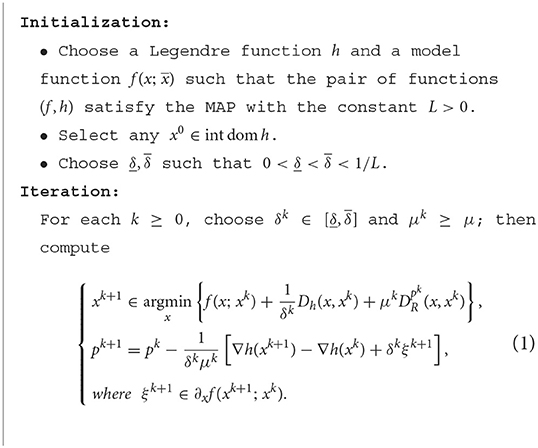
Algorithm 1. Bregman iterative regularization using model functions.

There are some remarks to understand ModelBI:

• First, note that ModelBI is a generalization of LBI. It replaces the linearized term of LBI with a model function that keeps the first-order information of f. For smooth f and model function f(x; x^k) = f(x^k) + 〈∇f(x^k), x − x^k〉, Algorithm 1 is actually the LBI algorithm in Zhang et al. [7].

• Denote ${{T}}_{x^k}(x):=f(x;x^k)+\frac{1}{{\delta }^k}{D}_h(x,x^k)+{\mu }^k{D}_R^{p^k}(x,x^k)$, then $\text{argmi}{\text{n}}_x{{T}}_{x^k}(x)$ is a set of minimizers. When $\text{argmi}{\text{n}}_x{{T}}_{x^k}(x)$ is a singleton, the update step becomes $x^{k+1}=\text{argmi}{\text{n}}_x{{T}}_{x^k}(x)$.

• A potential problem is the choice of ξ^k+1 if the model function is also nonsmooth. We need to pick a specific element from the set ${\partial }_{x}f(x^{k+1};x^k)$ for this case. Corollary 4.7 shows that a random element from ${\partial }_{x}f(x^{k+1};x^k)$ is acceptable as ξ^k → 0 (k → ∞) under some standard assumptions. Section 6 further verifies this strategy via numerical experiments.

4. Global convergence analysis

In this section, we analyze the convergence of the ModelBI algorithm. We first present that our algorithm results in monotonically nonincreasing function values.

Lemma 4.1 (Sufficient descent property of {f(x^k)}). Let Assumption 3.1 hold and {x^k} be a sequence generated by the ModelBI algorithm; then for k ≥ 0, we have that

$\begin{array}{ll}f(x^{k+1})\le f(x^k)-{\epsilon }^k{D}_h(x^{k+1},x^k)-{\mu }^k{D}_R^{p^k}(x^{k+1},x^k),& (2)\end{array}$

where ${\epsilon }^k=\frac{1}{{\delta }^k}-L$. In particular,

$\begin{array}{ll}{\displaystyle \underset{k\to \infty }{lim}}{D}_h(x^{k+1},x^k)={\displaystyle \underset{k\to \infty }{lim}}{D}_R^{p^k}(x^{k+1},x^k)=0.& (3)\end{array}$

Proof. Due to Equation (1), we have

$\begin{array}{l}f(x^{k+1};x^k)\le f(x^k;x^k)-\frac{1}{{\delta }^k}{D}_h(x^{k+1},x^k)-{\mu }^k{D}_R^{p^k}(x^{k+1},x^k).\end{array}$

From the MAP,

$\begin{array}{l}\begin{array}{l}f(x^{k+1})\le f(x^{k+1};x^k)+L{D}_h(x^{k+1},x^k)\\ \le f(x^k;x^k)-\frac{1}{{\delta }^k}{D}_h(x^{k+1},x^k)-{\mu }^k{D}_R^{p^k}(x^{k+1},x^k)\\ +L{D}_h(x^{k+1},x^k)\\ =f(x^k)-{\epsilon }^k{D}_h(x^{k+1},x^k)-{\mu }^k{D}_R^{p^k}(x^{k+1},x^k).\end{array}\end{array}$

where the last equality follows from the definition of the model function. As ${\epsilon }^k=\frac{1}{{\delta }^k}-L>0$, we obtain the sufficient descent property in function values.

Summing Equation (2) from k = 0 to n we get

$\begin{array}{l}{\displaystyle \sum _{k=0}^n}\left((\frac{1}{\overline{\delta }}-L)D_h(x^{k+1},x^k)+\mu D_R^{p^k}(x^{k+1},x^k)\right)\le f(x^0)\\ -f(x^{n+1})\le f(x^0)-{\displaystyle \underset{x\in \text{dom }h}{inf}}f(x).& (4)\end{array}$

Taking the limit as n → ∞, we obtain ${\sum }_{k=0}^{\infty }{D}_h(x^{k+1},x^k)<\infty$ and ${\sum }_{k=0}^{\infty }{D}_R^{p^k}(x^{k+1},x^k)<\infty$, from which we deduce that

$\begin{array}{l}{\displaystyle \underset{k\to \infty }{lim}}{D}_h(x^{k+1},x^k)={\displaystyle \underset{k\to \infty }{lim}}{D}_R^{p^k}(x^{k+1},x^k)=0.\end{array}$

This completes the proof.

To further show the convergence of the sufficient desent sequence {f(x^k)}, we now define the set of all limit points of {x^k} as follows

$\begin{array}{l}\Omega :=\\ \left\{\begin{array}{c}{x}^{*}\in {ℝ}^d:\text{there exists an increasing integer sequence}\left\{k_i\right\}\\ \text{such that }{\displaystyle {lim}_{i\to \infty }}{x}^{k_i}=x^{*}\end{array}\right\}.\end{array}$

Lemma 4.2 (Function value convergence). Let the same assumptions hold true as in Lemma 4.1. Suppose further that Assumption 3.2 holds, that h is strongly convex on dom h with dom h = dom h and that the level set {x : f(x) ≤ f(x⁰)} is bounded. Then, Ω ≠ ∅ and for any limit point x* ∈ Ω,

$\begin{array}{ll}{\displaystyle \underset{k\to \infty }{lim}}f(x^k)=f(x^{*}).& (5)\end{array}$

Proof. The boundness of {x:f(x) ≤ f(x⁰)} and the sufficient descent property of {f(x^k)} ensure the boundedness of {x^k}, hence Ω ≠ ∅.

Take x* ∈ Ω. There exists a subsequence $\left\{x^{k_i}\right\}\subset \left\{x^k\right\}\subset \text{int dom }h$ such that ${lim}_{i\to \infty }{x}^{k_i}=x^{*}\in \overline{\text{dom }h}=\text{dom }h$. Together with (3) in Lemma 4.1 and the strong convexity of h, we can conclude that $||x^{k_i+1}-x^{k_i}||\to 0$ and $||x^{k_i+1}-x^{*}||\to 0$ as i → ∞.

In light of (1), we have

$\begin{array}{l}\begin{array}{l}f(x^{k_i+1};x^{k_i})+\frac{1}{{\delta }^{k_i}}{D}_h(x^{k_i+1},x^{k_i})+{\mu }^{k_i}{D}_R^{p^{k_i}}(x^{k_i+1},x^{k_i})\\ \le f(x^{*};x^{k_i})+\frac{1}{{\delta }^{k_i}}{D}_h(x^{*},x^{k_i})+{\mu }^{k_i}{D}_R^{p^{k_i}}(x^{*},x^{k_i}).\end{array}\end{array}$

The MAP yields $f(x^{k_i+1})\le f(x^{k_i+1};x^{k_i})+L{D}_h(x^{k_i+1},x^{k_i})$. As ${\epsilon }^{k_i}=\frac{1}{{\delta }^{k_i}}-L>0$,

$\begin{array}{l}f(x^{k_i+1})\le f(x^{*};x^{k_i})+\frac{1}{{\delta }^{k_i}}{D}_h(x^{*},x^{k_i})+{\mu }^{k_i}{D}_R^{p^{k_i}}(x^{*},x^{k_i}).\end{array}$

Thus, we have

$\begin{array}{l}{\displaystyle \underset{i\to \infty }{lim}}supf(x^{k_i+1})\le f(x^{*};x^{*})=f(x^{*}).\end{array}$

Using the lsc property of f, we obtain

$\begin{array}{l}f(x^{*})\le {\displaystyle \underset{i\to \infty }{lim}}inff(x^{k_i+1}).\end{array}$

Therefore, we get

$\begin{array}{l}{\displaystyle \underset{i\to \infty }{lim}}f(x^{k_i+1})=f(x^{*}).\end{array}$

Note that {f(x^k)} is also lower bounded by ${inf}_{x\in \text{dom }h}f(x)$ and hence it is convergent. Then we have ${lim}_{k\to \infty }f(x^k)=f(x^{*})$, which completes the proof.

In order to derive the global convergence of {x^k}, we should introduce a modified surrogate function F : ℝ^d × ℝ^d × ℝ^d → (−∞, +∞]:

$\begin{array}{ll}F(x,y,z)=f(x;y)+L{D}_h(x,y)+\mu (R(x)+R^{*}(z)-\langle z,x\rangle ),& (6)\end{array}$

where R* is the convex conjugate of R.

Remark 1. The modified surrogate function is inspired by Benning et al. [6] and Zhang et al. [7]. However, their surrogate functions are invalid for our global convergence analysis, because the standard assumptions do not contain the subgradient relationship between the nonsmooth f and the model function. Thus, we replace the loss function with a Lyapunov function f(x; y) + LD_h(x, y) that appeared in Mukkamala et al. [10] to construct a new one. The new surrogate function imposes an additional variable, where we should make a mild assumption about the lower bound of the subgradient with respect to this variable (refer to Assumption 3.4). In addition, we have known that the Lyapunov function is a KL function [10]. As is mentioned in Section 2, the KL property holds under finite sums, which verifies that the proposed surrogate function (6) is also a KL function.

In the following, we present the sufficient descent property of F and its subgradient bounds, which are the basis of the convergence analysis. To this end, we introduce the notation s^k: = (x^k, x^k−1, p^k−1) for all k ∈ ℕ, and thus F(s^k) = F(x^k, x^k−1, p^k−1).

Lemma 4.3 (Sufficient descent property of {F(s^k)}). Let the same assumptions hold true as in Lemma 4.1 and μ^k ≥ μ ≥ 0. Then we have the following decent estimate:

$\begin{array}{l}F(s^{k+1})\le F(s^k)-{\epsilon }^k{D}_h(x^{k+1},x^k)-({\mu }^k-\mu )D_R^{p^k}(x^{k+1},x^k)\\ -\mu D_R^{p^{k-1}}(x^k,x^{k-1}).& (7)\end{array}$

Proof. Similar to the proof of Lemma 4.1, we have $f(x^{k+1};x^k)\le f(x^k)-\frac{1}{{\delta }^k}{D}_h(x^{k+1},x^k)-{\mu }^k{D}_R^{p^k}(x^{k+1},x^k)$ due to Equation (1), and $f(x^k)\le f(x^k;x^{k-1})+L{D}_h(x^k;x^{k-1})$ from the MAP. Note that $F(s^{k+1})=f(x^{k+1};x^k)+L{D}_h(x^{k+1},x^k)+\mu D_R^{p^k}(x^{k+1},x^k)$ for x^k ∈ ∂R*(p^k). Hence, combining the above formulas, we derive that

$\begin{array}{l}\begin{array}{l}F(s^{k+1})\le f(x^k)-{\epsilon }^k{D}_h(x^{k+1},x^k)-({\mu }^k-\mu )D_R^{p^k}(x^{k+1},x^k)\\ \le f(x^k;x^{k-1})+L{D}_h(x^k;x^{k-1})-{\epsilon }^k{D}_h(x^{k+1},x^k)\\ -({\mu }^k-\mu )D_R^{p^k}(x^{k+1},x^k)\\ =F(s^k)-{\epsilon }^k{D}_h(x^{k+1},x^k)-({\mu }^k-\mu )D_R^{p^k}(x^{k+1},x^k)\\ -\mu D_R^{p^{k-1}}(x^k,x^{k-1}),\end{array}\end{array}$

which completes the proof.

Remark 2. From the definition of the surrogate function, we know that $F(s^k)\ge f(x^k)\ge {inf}_{x\in \text{dom }h}f(x)\ge -\infty$. Together with the sufficient decent property, the sequence {F(s^k)} is also bounded.

Note that the subdifferential of the surrogate function reads as

$\begin{array}{l}\partial F(x,y,z)=\left(\begin{array}{c}{\partial }_{x}f(x;y)+L(\nabla h(x)-\nabla h(y))+\mu \partial R(x)-\mu z\\ {\partial }_{y}f(x;y)-L{\nabla }^{2}h(y)(x-y)\\ \mu (\partial R^{*}(z)-x)\end{array}\right).\end{array}$

Then, a lower bound for its subgradients at the iterates computed with ModelBI can be deduced.

Lemma 4.4 (Subgradient lower bound of F(s^k)). Let the same assumptions hold true as in Lemma 4.3. Suppose further that Assumption 3.3 holds for h and Assumption 3.4 holds for f. Then the subgradient is lower bounded by the iterates gap:

$\begin{array}{l}||\partial F(x^{k+1},x^k,p^k)|{|}_{-}\le (\frac{L_h}{{\delta }^k}+\mu +c)||x^{k+1}-x^k||\\ +({\mu }^k-\mu )||p^{k+1}-p^k||.& (8)\end{array}$

Proof. Using the fact that p^k+1 ∈ ∂R(x^k+1) and x^k ∈ ∂R*(p^k), we know

$\begin{array}{ll}\begin{array}{l}||\partial F(x^{k+1},x^k,p^k)|{|}_{-}\le {\displaystyle \underset{\xi \in {\partial }_{x}f(x^{k+1};x^k)}{inf}}||\xi +L(\nabla h(x^{k+1})\\ -\nabla h(x^k))+\mu (p^{k+1}-p^k)||\\ +{\displaystyle \underset{\eta \in {\partial }_{y}f(x^{k+1};x^k)}{inf}}||\eta -L{\nabla }^{2}h(x^k)(x^{k+1}-x^k)||\\ +\mu ||x^{k+1}-x^k||.\end{array}& (9)\end{array}$

The optimality of x^k+1 in Equation (1) implies the existence of ${\xi }^{k+1}\in {\partial }_{x}f(x^{k+1};x^k)$ such that the following condition holds: ${\xi }^{k+1}+\frac{1}{{\delta }^k}(\nabla h(x^{k+1})-\nabla h(x^k))+{\mu }^k(p^{k+1}-p^k)=0$. Then the first term of the right hand side in Equation (9) is bounded by

$\begin{array}{l}\begin{array}{l}{\displaystyle \underset{\xi \in {\partial }_{x}f(x^{k+1};x^k)}{inf}}||\xi +L(\nabla h(x^{k+1})-\nabla h(x^k))+\mu (p^{k+1}-p^k)||\\ \le (\frac{1}{{\delta }^k}-L)||\nabla h(x^{k+1})-\nabla h(x^k)||+({\mu }^k-\mu )||p^{k+1}-p^k||\\ \le (\frac{1}{{\delta }^k}-L)L_h||x^{k+1}-x^k||+({\mu }^k-\mu )||p^{k+1}-p^k||,\end{array}\end{array}$

where in the last inequality we applied the Lagrange mean value theorem along with the fact that the entity ∇²h(x^k+1 + s(x^k+1 − x^k)) (s ∈ [0, 1]) is bounded by a constant L_h. Considering the second term in Equation (9), we have

$\begin{array}{l}\begin{array}{l}{\displaystyle \underset{\eta \in {\partial }_{y}f(x^{k+1};x^k)}{inf}}||\eta -L{\nabla }^{2}h(x^k)(x^{k+1}-x^k)||\\ \le {\displaystyle \underset{\eta \in {\partial }_{y}f(x^{k+1};x^k)}{inf}}||\eta ||+L||{\nabla }^{2}h(x^k)||||x^{k+1}-x^k||\\ \le c||x^{k+1}-x^k||+L{L}_h||x^{k+1}-x^k||,\end{array}\end{array}$

where in the last inequality we used Assumption 3.4 and the fact that ||∇²h(x^k)|| is bounded by L_h. Note that there is no loss of generality to take the same L_h as the upper bound. We therefore estimate

$\begin{array}{l}||\partial F(x^{k+1},x^k,p^k)|{|}_{-}\le \\ (\frac{L_h}{{\delta }^k}+\mu +c)||x^{k+1}-x^k||\\ +({\mu }^k-\mu )||p^{k+1}-p^k||.\end{array}$

This completes the proof.

Recall that {s^k} = {(x^k, x^k−1, p^k−1)} is a sequence generated by ModelBI from starting points x⁰ and p⁰. Denote the set of limit points of {s^k} as

$\begin{array}{l}{\Omega }_0:=\\ \left\{\begin{array}{c}{s}^{*}=(x^{*},x^{*},p^{*})\in {ℝ}^d\times {ℝ}^d\times {ℝ}^d:\text{there exists an increasing integer sequence}\\ \left\{k_i\right\}\text{ such that }{\displaystyle {lim}_{i\to \infty }}{x}^{k_i}=x^{*},{\displaystyle {lim}_{i\to \infty }}{x}^{k_i-1}=x^{*},\text{ and }{\displaystyle {lim}_{i\to \infty }}{p}^{k_i-1}=p^{*}\end{array}\right\}.\end{array}$

Before we show the global convergence of the ModelBI sequence to a critical point of f, we need to verify that (i) Ω₀ is a nonempty, compact, and connected set, and (ii) the surrogate function F converges to f on Ω₀. Both of them are guaranteed by the following lemma.

Lemma 4.5 (Function value convergence of {F(s^k)}). Under the conditions of Lemma 4.4, let Assumption 3.2 hold and Assumption 3.5 hold for R. Suppose that ${lim}_{k\to \infty }{\mu }^k=\mu$, that h is strongly convex on dom h with dom h = dom h, and that the level set {x:f(x) ≤ f(x⁰)} is bounded. Then Ω₀ is a nonempty, compact, and connected set, and for any $s^{*}=(x^{*},x^{*},p^{*})\in {\Omega }_0$, we have ${lim}_{k\to \infty }\text{dist}(s^k,{\Omega }_0)=0$ and

$\begin{array}{l}{\displaystyle \underset{k\to \infty }{lim}}F(s^k)=f(x^{*}).\end{array}$

Proof. By the boundedness of {x^k}, there exists an increase of integers {i_j}_j∈ℕ such that ${lim}_{j\to \infty }{x}^{i_j}=x^{*}$. With $p^{i_j}\in \partial R(x^{i_j})$ and the subgradient local boundedness of R(x), we know that $\left\{p^{i_j}\right\}$ must be bounded, and thus, there exists a subsequence {k_i} ⊂ {i_j} such that ${lim}_{i\to \infty }{p}^{k_i}=\overline{p}$. Due to Equation (1), it holds that

$\begin{array}{l}{\mu }^{k_i-1}{p}^{k_i}={\mu }^{k_i-1}{p}^{k_i-1}-\frac{1}{{\delta }^{k_i-1}}(\nabla h(x^{k_i})-\nabla h(x^{k_i-1}))-{\xi }^{k_i}.\end{array}$

Due to Equation (3) in Lemma 4.1 and the strong convexity of h, we know that ${lim}_{i\to \infty }{x}^{k_i}={lim}_{i\to \infty }{x}^{k_i-1}=x^{*}$ and ${lim}_{i\to \infty }{\xi }^{k_i}={\xi }^{*}\in {\partial }_{x}f(x^{*};x^{*})$. Together with ${lim}_{i\to \infty }{\mu }^{k_i-1}=\mu$ and the boundedness of $\left\{{\delta }^{k_i-1}\right\}$, we conclude that there exists a point p* such that ${lim}_{i\to \infty }{p}^{k_i-1}=p^{*}$ (p* may be different to $\overline{p}$). Therefore, s* = (x*, x*, p*) indeed belongs to Ω₀ which shows the nonemptiness of Ω₀. Furthermore, x* ∈ Ω for each $s^{*}\in {\Omega }_0$.

From Theorem 3.7 in Rubin [22], the set Ω₀ must be closed since it is the set of cluster points of {s^k}. The boundedness of Ω₀ comes from the boundedness of {x^k} and {p^k}. Therefore, the set Ω₀ is compact and hence ${lim}_{k\to \infty }\text{dist}(s^k,{\Omega }_0)=0$ by the definition of limit points.

Note that by definition of F we have

$\begin{array}{l}\begin{array}{l}F(s^k)=f(x^k;x^{k-1})+L{D}_h(x^k,x^{k-1})+\mu D_R^{p^{k-1}}(x^k,x^{k-1})\\ =f(x^k)+\left(f(x^k;x^{k-1})-f(x^k)\right)+L{D}_h(x^k,x^{k-1})\\ +\mu D_R^{p^{k-1}}(x^k,x^{k-1}).\end{array}\end{array}$

The MAP gives $f(x^k)\le F(s^k)\le f(x^k)+2L{D}_h(x^k,x^{k-1})+\mu D_R^{p^{k-1}}(x^k,x^{k-1})$. As ${lim}_{k\to \infty }{D}_h(x^k,x^{k-1})={lim}_{k\to \infty }{D}_R^{p^{k-1}}(x^k,x^{k-1})=0$ in Lemma 4.1 and ${lim}_{k\to \infty }f(x^k)=f(x^{*})$ in Lemma 4.2, we deduce that

$\begin{array}{l}{\displaystyle \underset{k\to \infty }{lim}}F(s^k)=f(x^{*}),\end{array}$

which completes the proof.

Now we are ready to present the following global convergence result for ModelBI.

Theorem 4.6 (Finite length property). Let {s^k} = {(x^k, x^k−1, p^k−1)} be the sequence generated by the ModelBI algorithm. Suppose that F is a KL function in the sense of Definition 2.4. Let Assumptions 3.1–3.2 hold, Assumption 3.3 hold for h, Assumption 3.4 hold for f, and Assumption 3.5 hold for R. In addition, let h be σ_h-strongly convex with dom h = dom h, the level set {x : f(x) ≤ f(x⁰)} is bounded, the parameters δ^k satisfy $0<\underset{\_}{\delta }\le {\delta }^k\le \overline{\delta }<1/L$, and μ^k satisfy μ^k ≥ μ and ${\sum }_{k=0}^{\infty }({\mu }^k-\mu )<\infty$. Then, the sequence {x^k} has a finite length in the sense that

$\begin{array}{ll}{\displaystyle \sum _{k=0}^{\infty }}||x^{k+1}-x^k||<\infty .& (10)\end{array}$

Proof. We show Equation (10) by modifying the methodology in Zhang et al. [7]. Let us begin with any point $s^{*}=(x^{*},x^{*},p^{*})\in {\Omega }_0$. Then, there exists an increasing integer sequence {k_i}_i∈ℕ such that $x^{k_i}\to x^{*}$ as i → ∞. From Lemma 4.5 and recalling that s^k = (x^k, x^k−1, p^k−1), we know ${lim}_{k\to \infty }F(s^k)=f(x^{*})$.

Note that the convergent sequence {F(s^k)} is nonincreasing from Lemma 4.3. If there exists an integer $\bar{k}$ such that $F(s^{\bar{k}})=f(x^{*})$, then F(s^k) ≡ f(x*) for $k\ge \bar{k}$ and hence $D_h(x^{k+1},x^k)=0$ for $k\ge \bar{k}$ from Equation (7), which implies that $x^k\equiv x^{\bar{k}}$ for $k\ge \bar{k}$ due to the strong convexity of h. Hence, the result (Equation 10) follows trivially. If there does not exist such an index, then F(s^k) > f(x*) holds for all k > 0. Since ${lim}_{k\to \infty }F(s^k)=f(x^{*})$, for any η > 0 there must exist an integer $\widehat{k}>0$ such that F(s^k) < f(x*) + η for all $k>\widehat{k}$. Similarly, ${lim}_{k\to \infty }\text{dist}(s^k,{\Omega }_0)=0$ from Lemma 4.5 implies for any ζ > 0 there must exist an integer $\tilde{k}>0$ such that $\text{dist}(s^k,{\Omega }_0)<\zeta$ for all $k>\tilde{k}$. Therefore, for all $k>l:=max\left\{\widehat{k},\tilde{k}\right\}$ we have

$\begin{array}{l}{s}^k\in \left\{s:\text{dist}(s,{\Omega }_0)<\zeta \right\}\bigcap \left\{s:f(x^{*})<F(s)<f(x^{*})+\eta \right\}.\end{array}$

Thus, we apply Definition 2.4 to get,

$\begin{array}{ll}{\phi }^{\prime }(F(s^k)-f(x^{*}))||\partial F(s^k)|{|}_{-}\ge 1.& (11)\end{array}$

Using Equation 4.4 in Lemma 4.4 and ${\delta }^k\in \left[\underset{\_}{\delta },\overline{\delta }\right]$, we get that

$\begin{array}{ll}||\partial F(s^k)|{|}_{-}\le \overline{\rho }||x^k-x^{k-1}||+({\mu }^{k-1}-\mu )||p^k-p^{k-1}||.& (12)\end{array}$

where $\overline{\rho }=\frac{L_h}{\underset{\_}{\delta }}+\mu +c$. On the other hand, from the concavity of φ, we know that

${\phi }^{\prime }(x)\le \frac{\phi (x)-\phi (y)}{x-y}$

holds for all x, y ∈ [0, η), x > y. Hence, by taking x = F(s^k) − f(x*) and y = F(s^k+1) − f(x*) in the inequality above, we get

$\begin{array}{ll}{\phi }^{\prime }(F(s^k)-f(x^{*}))\le \frac{{\phi }^k-{\phi }^{k+1}}{F(s^k)-F(s^{k+1})}\le \frac{2({\phi }^k-{\phi }^{k+1})}{\underset{\_}{\epsilon }{\sigma }_h||x^{k+1}-x^k|{|}^2},& (13)\end{array}$

where φ^k: = φ(F(s^k) − f(x*)) and $\underset{\_}{\epsilon }=\frac{1}{\overline{\delta }}-L$. The last inequality follows from Equation (7) and the strong convexity property $D_h(x^{k+1},x^k)\ge \frac{{\sigma }_h}{2}||x^{k+1}-x^k|{|}^2$. Therefore, from Equations (11)–(13), we get

$\begin{array}{l}||x^{k+1}-x^k|{|}^2\le \frac{2\overline{\rho }}{\underset{\_}{\epsilon }{\sigma }_h}\left({\phi }^k-{\phi }^{k+1}\right)(||x^k-x^{k-1}||\\ +\frac{{\mu }^{k-1}-\mu }{\overline{\rho }}||p^k-p^{k-1}||).\end{array}$

Based on Young's inequality of form $2\sqrt{ab}\le a+b$, we further get

$\begin{array}{l}2||x^{k+1}-x^k||\le \frac{2\overline{\rho }}{\underset{\_}{\epsilon }{\sigma }_h}({\phi }^k-{\phi }^{k+1})+||x^k-x^{k-1}||\\ +\frac{{\mu }^{k-1}-\mu }{\overline{\rho }}||p^k-p^{k-1}||.\end{array}$

Subtracting ||x^k+1 − x^k|| and summing the inequality above from k = l, ⋯ , N yields

$\begin{array}{l}{\displaystyle \sum _{k=l}^N}||x^{k+1}-x^k||\le ||x^l-x^{l-1}||+{\displaystyle \sum _{k=l}^N}\frac{{\mu }^{k-1}-\mu }{\overline{\rho }}||p^k-p^{k-1}||\\ +\frac{2\overline{\rho }}{\underset{\_}{\epsilon }{\sigma }_h}({\phi }^l-{\phi }^{N+1}).\end{array}$

With the boundedness of {p^k} and ${\sum }_{k=0}^{\infty }({\mu }^k-\mu )$, we obtain the finite length property by letting N → ∞.

Corollary 4.7. Under the same assumptions as Theorem 4.6, the sequence {x^k} converges to a critical point of f in the sense that 0 ∈ ∂f(x*). In addition, we have the following rate of convergence result:

$\begin{array}{ll}{\displaystyle \underset{0\le k\le n}{min}}||x^{k+1}-x^k|{|}^2\le \frac{1}{n}·\frac{2\overline{\delta }}{{\sigma }_h(1-\overline{\delta }L)}\left(f(x^0)-f(x^{*})\right).& (14)\end{array}$

Proof. The finite length property Theorem 4.6 implies that ${\sum }_{k=l}^{\infty }||x^{k+1}-x^k||\to 0$ as l → ∞. Thus, for any m > n ≥ l we have

$\begin{array}{l}||x^m-x^n||=\left|\right|{\displaystyle \sum _{k=n}^{m-1}}(x^{k+1}-x^k)\left|\right|\le {\displaystyle \sum _{k=n}^{m-1}}||x^{k+1}-x^k||\\ \le {\displaystyle \sum _l^{\infty }}||x^{k+1}-x^k||,\end{array}$

which implies that {x^k} is a Cauchy sequence. ModelBI gives

$\begin{array}{l}{p}^k-p^{k+1}=\frac{1}{{\delta }^k{\mu }^k}\left(\nabla h(x^{k+1})-\nabla h(x^k)\right)+\frac{1}{{\mu }^k}{\xi }^{k+1}.\end{array}$

Summing from k = 0, ⋯ , n leads to

$\begin{array}{l}{p}^0-p^{n+1}={\displaystyle \sum _{k=0}^n}\left(\frac{1}{{\delta }^k{\mu }^k}\left(\nabla h(x^{k+1})-\nabla h(x^k)\right)+\frac{1}{{\mu }^k}{\xi }^{k+1}\right).\end{array}$

Assume that the limit point ξ* ≠ 0. Noting that $\frac{1}{{\delta }^k{\mu }^k}\left(\nabla h(x^{k+1})-\nabla h(x^k)\right)\to 0$ and $\frac{1}{{\mu }^k}{\xi }^{k+1}\to \frac{1}{\mu }{\xi }^{*}\ne 0$, we apply Lemma 4.8 in Zhang et al. [7] to conclude that ||p⁰ − pⁿ⁺¹|| → ∞ as n → ∞, which contradicts the boundedness of {p^k}. Therefore, we have ξ* = 0 ∈ ∂f(x*).

Recalling (4) in Lemma 4.1, we have

$\begin{array}{l}{\displaystyle \underset{0\le k\le n}{min}}{D}_h(x^{k+1},x^k)\le \frac{1}{n}·\frac{\overline{\delta }}{1-\overline{\delta }L}\left(f(x^0)-f(x^{*})\right),\end{array}$

which immediately leads to the result of a convergence rate due to the strong convexity of h.

5. Application to phase retrieval problems

This section illustrates the potential of the proposed algorithm. To this end, we consider two kinds of nonsmooth phase retrieval problems and construct the corresponding model functions that the MAP holds. Then, we show how ModelBI can be applied to these problems.

The standard phase retrieval problem can be described as follows. Given a finite number of measurement vectors $a_i\in {ℝ}^d,i=1,2,...,m$, describing the model, and a vector b ∈ ℝ^m describing the possibly corrupted measurement data, our goal is to find x ∈ ℝ^d that solves the system

$\begin{array}{ll}|\langle a_i,x\rangle |\simeq b_i,i=1,2,...,m.& (15)\end{array}$

It is a natural extension of the standard linear inverse problem, as the linear measurements are replaced by their modules. This type of problem has been and is still being intensively studied in the literature; readers can refer to Dong et al. [23] for a brief review.

The considered system (Equation 15) is commonly underdetermined, and thus some prior information of the target vector is brought into the model by means of some regularizer R. Adopting the usual mean-value or least-square loss function f to measure the error, the problem can be reformulated in the form of (${P}$). What we are concerned about are the following two nonsmooth models:

(A) Mean-value loss function with intensity-only measurements [24], i.e.,

$\begin{array}{l}f(x)=\frac{1}{m}{\displaystyle \sum _{i=1}^m}|{\langle a_i,x\rangle }^2-b_i^2|.\end{array}$

(B) Least-square loss function with amplitude-only measurements [25], i.e.,

$\begin{array}{l}f(x)=\frac{1}{m}{\displaystyle \sum _{i=1}^m}{(|\langle a_i,x\rangle |-b_i)}^2.\end{array}$

For simplicity and generalization, in both cases (A) and (B), we use the Legendre function $h(x)=\frac{1}{2}||x|{|}^2$ and the convex ℓ₁-norm regularization R(x) = ||x||₁.

5.1. Model A

With the usual mean-value loss function, we can reformulate (Equation 15) as the following nonconvex nonsmooth optimization problem

$\begin{array}{l}{\displaystyle \underset{x\in {ℝ}^d}{min}}\left\{\frac{1}{m}{\displaystyle \sum _{i=1}^m}|x^T{A}_{i}x-b_i^2|+\mu R(x)\right\},\end{array}$

where $A_i=a_i{a}_i^T$, i = 1, …, m are symmetric matrices.

To apply ModelBI to this model, we first need to identify an appropriate model function such that the MAP holds for the pair (f, h). Consider the composite function $f(G(x))=\frac{1}{m}{\sum }_{i=1}^m|x^T{A}_{i}x-b_i^2|$, where $f(·)=\frac{1}{m}||·|{|}_1$ and $G_i(x)=x^T{A}_{i}x-b_i^2$ for all i = 1, …, m. The structure of f(G(x)) enables us to construct the model function as follows:

$\begin{array}{ll}f(x;x^k)=\frac{1}{m}{\displaystyle \sum _{i=1}^m}|G_i(x^k)+\langle \nabla G_i(x^k),x-x^k\rangle |,& (16)\end{array}$

where $\nabla G_i(x^k)=2A_i{x}^k$. With $h(x)=\frac{1}{2}||x|{|}^2$, we now show that there exists L > 0 such that $|f(G(x))-f(x;x^k)|\le L{D}_h(x,x^k)$.

Proposition 5.1. Let f, G, h, and the model function be as defined above. Then, for any L satisfying

$\begin{array}{l}L\ge \frac{2}{m}{\displaystyle \sum _{i=1}^m}||A_i|{|}_F,\end{array}$

the MAP holds for the function pair (f, h).

Proof. Let x ∈ ℝ^d and x^k be the current iterate. Since G is ${{C}}^1$ on ℝ^d, we obtain the following model function by straightly computing:

$\begin{array}{l}f(x;x^k)=\frac{1}{m}{\displaystyle \sum _{i=1}^m}|\left({(x^k)}^T{A}_i{x}^k-b_i^2\right)+\langle 2A_i{x}^k,x-x^k\rangle |.\end{array}$

Then, the error between the loss function and the model function is quantified by

$\begin{array}{l}\begin{array}{l}|f(G(x))-f(x;x^k)|\le \frac{1}{m}{\displaystyle \sum _{i=1}^m}|G_i(x)-G_i(x^k)-\langle \nabla G_i(x^k),x-x^k\rangle |\\ =\frac{1}{m}{\displaystyle \sum _{i=1}^m}|\left(x^T{A}_{i}x-b_i^2\right)-\left({(x^k)}^T{A}_i{x}^k-b_i^2\right)-\langle 2A_i{x}^k,x-x^k\rangle |\\ =\frac{1}{m}{\displaystyle \sum _{i=1}^m}\left|{(x-x^k)}^T{A}_i(x-x^k)\right|\\ \le \frac{1}{m}{\displaystyle \sum _{i=1}^m}||A_i|{|}_F||x-x^k|{|}^2\end{array}\end{array}$

Note that h is strongly convex and $D_h(x,x^k)=\frac{1}{2}||x-x^k|{|}^2$. Therefore, taking $L\ge \frac{2}{m}{\sum }_{i=1}^m||A_i|{|}_F$ yields $|f(G(x))-f(x;x^k)|\le L{D}_h(x,x^k)$, which proves the desired result.

It is straightforward to verify that the setting implies Assumptions 3.1–3.5. Thus, the sequence {x^k} generated by ModelBI globally converges to a critical point of f due to Corollary 4.7. With the notation ${\overline{p}}^k=-\nabla h(x^k)-{\delta }^k{\mu }^k{p}^k$, we can rewrite the main computational gradient map in Equation (1) as follows

$\begin{array}{ll}{x}^{k+1}={\displaystyle \underset{x}{\text{argmin}}}\left\{{\delta }^{k}f(x;x^k)+{\delta }^k{\mu }^{k}R(x)+\langle {\overline{p}}^k,x\rangle +h(x)\right\}.& (17)\end{array}$

Observing that there are two nonsmooth terms in this subproblem, it is difficult to deduce the closed form solutions. Here, we propose the alternating direction method of multipliers (ADMM) as a choice.

Let $H(x)={\delta }^k{\mu }^{k}R(x)+\langle {\overline{p}}^k,x\rangle +h(x)$ and $I(y)=\frac{{\delta }^k}{m}||y|{|}_1$; then the subproblem (Equation 17) can be reformulated as the 2-block optimization problem

$\begin{array}{l}\begin{array}{l}{\displaystyle \underset{x,y}{\text{minimize}}}H(x)+I(y),\\ \text{ s}.\text{t}.G_i(x^k)+\langle \nabla G_i(x^k),x-x^k\rangle -y_i=0,i=1,...,m.\end{array}\end{array}$

With a regular parameter ρ and a vector z ∈ ℝ^m, the Augmented Lagrangian function for the reformulated problem is

$\begin{array}{ll}\begin{array}{l}{L}_{\rho }(x,y,z)=H(x)+I(y)\\ +{\displaystyle \sum _{i=1}^m}{z}_i\left(G_i(x^k)+\langle \nabla G_i(x^k),x-x^k\rangle -y_i\right)\\ +\frac{\rho }{2}{\displaystyle \sum _{i=1}^m}{\left(G_i(x^k)+\langle \nabla G_i(x^k),x-x^k\rangle -y_i\right)}^2.\end{array}& (18)\end{array}$

Based on the dual ascent method, ADMM separates the variants of L_ρ(x, y, z) and iterates alternately by the following scheme:

$\begin{array}{l}\{\begin{array}{l}{y}^{k+1}={\displaystyle \underset{y}{\text{argmin }}}{L}_{\rho }(x^k,y,z^k),\\ x^{k+1}={\displaystyle \underset{x}{\text{argmin }}}{L}_{\rho }(x,y^{k+1},z^k),\\ z_i^{k+1}=z_i^k+\rho \left(G_i(x^k)+\langle \nabla G_i(x^k),x^{k+1}-x^k\rangle -y_i^{k+1}\right),\\ i=1,...,m.\end{array}\end{array}$

With the well-known soft-thresholding operator S_τ(·) = max{| · | − τ, 0}sgn(·), the ADMM scheme admits explicit iteration steps. Here, we present the derived results below for computation:

$\begin{array}{l}\{\begin{array}{l}{y}^{k+1}=S_{\frac{{\delta }^k}{\rho m}}\left(G(x^k)+\frac{1}{\rho }{z}^k\right),\\ x^{k+1}=S_{\frac{{\delta }^k{\mu }^k{\eta }^k}{1+{\eta }^k}}(\frac{\rho {\eta }^k}{1+{\eta }^k}{\displaystyle \sum _{i=1}^m}(y_i^{k+1}-G_i(x^k)-\frac{1}{\rho }{z}_i^k)\nabla G_i(x^k)\\ -\frac{{\eta }^k}{1+{\eta }^k}{\overline{p}}^k+\frac{1}{1+{\eta }^k}{x}^k),\\ z_i^{k+1}=z_i^k+\rho \left(G_i(x^k)+\langle \nabla G_i(x^k),x^{k+1}-x^k\rangle -y_i^{k+1}\right),\\ i=1,...,m,\end{array}\end{array}$

where the solution of the first variant x^k+1 is derived by linearized ADMM (L-ADMM) [26] for the quadratic regularization term in Equation (18), and η^k is the stepsize.

Remark 3. We utilized ADMM with single-step iteration to solve the first subproblems of both nonsmooth models. As the finite length property ensures the global convergence of our proposed algorithm, we do not need a high-accuracy solution from ADMM in each iteration.

5.2. Model B

Another nonconvex nonsmooth optimization problem in phase retrieval is recovering a solution from the amplitude-based objective [25]. With the least-squared criterion and amplitude-only measurements, we can reformulate (Equation 15) as follows:

$\begin{array}{l}{\displaystyle \underset{x\in {ℝ}^d}{min}}\left\{\frac{1}{m}{\displaystyle \sum _{i=1}^m}{(|\langle a_i,x\rangle |-b_i)}^2+\mu R(x)\right\}.\end{array}$

To apply ModelBI as Model A, we first need to handle the loss function $f(x)=\frac{1}{m}{\sum }_{i=1}^m{(|\langle a_i,x\rangle |-b_i)}^2$. The structure is totally different from that of Model A as the inner functions |〈a_i, x〉| are nonsmooth. Thus, the linearized technique is not feasible for its model function. Fortunately, by considering the equivalent form of amplitude $\sqrt{{\langle a_i,x\rangle }^2}$ and adding an error term at the current iterate, we construct its model function that satisfies the MAP with the Legendre function $h(x)=\frac{1}{2}||x|{|}^2$:

$\begin{array}{ll}f(x;x^k)=\frac{1}{m}{\displaystyle \sum _{i=1}^m}{\left(\sqrt{{\langle a_i,x\rangle }^2+\frac{1}{4}{\langle a_i,x-x^k\rangle }^4}-b_i\right)}^2& (19)\end{array}$

Proposition 5.2. Let f, h, and the model function be as defined above. Assume that the error around the current iterate satisfies ||x − x^k|| ≤ 1. Then, for any L satisfying

$\begin{array}{l}L\ge \frac{2}{m}{\displaystyle \sum _{i=1}^m}\left(b_i+\frac{1}{4}||a_i|{|}^2\right)||a_i|{|}^2,\end{array}$

the MAP holds for the function pair (f, h).

Proof. Let x ∈ ℝ^d and x^k be the current iterate. We obtain the error between the loss function and the model function by straightly computing:

$\begin{array}{l}\begin{array}{l}|f(x)-f(x;x^k)|\le \frac{1}{m}{\displaystyle \sum _{i=1}^m}|{\left(\sqrt{{\langle a_i,x\rangle }^2}-b_i\right)}^2\\ -{\left(\sqrt{{\langle a_i,x\rangle }^2+\frac{1}{4}{\langle a_i,x-x^k\rangle }^4}-b_i\right)}^2|\\ =\frac{1}{m}{\displaystyle \sum _{i=1}^m}|2b_i\left(\sqrt{{\langle a_i,x\rangle }^2+\frac{1}{4}{\langle a_i,x-x^k\rangle }^4}-\sqrt{{\langle a_i,x\rangle }^2}\right)\\ -\frac{1}{4}{\langle a_i,x-x^k\rangle }^4|\\ \le \frac{1}{m}{\displaystyle \sum _{i=1}^m}(2b_i\left(\sqrt{{\langle a_i,x\rangle }^2+\frac{1}{4}{\langle a_i,x-x^k\rangle }^4}-\sqrt{{\langle a_i,x\rangle }^2}\right)\\ +\frac{1}{4}{\langle a_i,x-x^k\rangle }^4)\\ \le \frac{1}{m}{\displaystyle \sum _{i=1}^m}\left(b_i||a_i|{|}^2||x-x^k|{|}^2+\frac{1}{4}||a_i|{|}^4||x-x^k|{|}^4\right)\\ \le \frac{1}{m}{\displaystyle \sum _{i=1}^m}(b_i+\frac{1}{4}||a_i|{|}^2)||a_i|{|}^2||x-x^k|{|}^2,\end{array}\end{array}$

where the third inequality comes from $\sqrt{{\langle a_i,x\rangle }^2+\frac{1}{4}{\langle a_i,x-x^k\rangle }^4}\le \sqrt{{\langle a_i,x\rangle }^2}+\frac{1}{2}{\langle a_i,x-x^k\rangle }^2$, and the last inequality comes from ||x − x^k|| ≤ 1. Note that h is strongly convex and $D_h(x,x^k)=\frac{1}{2}||x-x^k|{|}^2$. Therefore, taking $L\ge \frac{2}{m}{\sum }_{i=1}^m(b_i+\frac{1}{4}||a_i|{|}^2)||a_i|{|}^2$ yields $|f(x)-f(x;x^k)|\le L{D}_h(x,x^k)$, which proves the desired result.

Remark 4. Our proposed model function (Equation 19) is inspired by the smoothing phase retrieval algorithm [25], in which each amplitude term |〈a_i, x〉| is smoothed by $\sqrt{{\langle a_i,x\rangle }^2+{\mu }^2}$ with μ ∈ ℝ₊₊. However, the smoothing term cannot be used as the model function, as it approximates |〈a_i, x〉| independent of x^k.

Remark 5. Note that the assumption that ||x − x^k|| ≤ 1 is not nontrivial. It can be satisfied by preconditioning the model data. For a certain random model, an initial vector x⁰ via the spectral method can reach sufficient accuracy with high probability [27].

It is straightforward to verify that Assumptions 3.1–3.5 holds. Thus, Corollary 4.7 imply that the sequence {x^k} generated by ModelBI globally converges to a critical point of f. With the notation ${\overline{p}}^k=-\nabla h(x^k)-{\delta }^k{\mu }^k{p}^k$, we can also rewrite the main computational gradient map as Equation (17).

Though the model function (Equation 19) is smooth, its structure still hinders us from obtaining the closed form solutions in the subproblem, which again needs the help of ADMM in the following.

Let $H(x)={\delta }^k{\mu }^{k}R(x)+\langle {\overline{p}}^k,x\rangle +h(x)$ and $I(y)=\frac{{\delta }^k}{m}||y|{|}^2$; then the subproblem (17) can be reformulated as the 2-block optimization problem

$\begin{array}{l}\begin{array}{l}{\displaystyle \underset{x,y}{\text{minimize}}}H(x)+I(y),\\ \text{ s}.\text{t}.\sqrt{{\langle a_i,x\rangle }^2+\frac{1}{4}{\langle a_i,x-x^k\rangle }^4}-b_i-y_i=0,\\ i=1,...,m.\end{array}\end{array}$

With a regular parameter ρ and a vector z ∈ ℝ^m, the Augmented Lagrangian function for the reformulated problem is

$\begin{array}{l}{L}_{\rho }(x,y,z)=H(x)+I(y)+{\displaystyle \sum _{i=1}^m}{z}_i({\sqrt{\langle }{a}_i,x\rangle }^2\\ +\frac{1}{4}{\langle a_i,x-x^k\rangle }^4-b_i-y_i)\\ +\frac{\rho }{2}{\displaystyle \sum _{i=1}^m}{\left(\sqrt{{\langle a_i,x\rangle }^2+\frac{1}{4}{\langle a_i,x-x^k\rangle }^4}-b_i-y_i\right)}^2.\end{array}$

Based on the dual ascent method, ADMM separates the variants of L_ρ(x, y, z) and iterates alternately by the following scheme:

$\begin{array}{l}\{\begin{array}{l}{y}^{k+1}={\displaystyle \underset{y}{\text{argmin }}}{L}_{\rho }(x^k,y,z^k),\\ x^{k+1}={\displaystyle \underset{x}{\text{argmin }}}{L}_{\rho }(x,y^{k+1},z^k),\\ z_i^{k+1}=z_i^k+\rho \left(\sqrt{{\langle a_i,x^{k+1}\rangle }^2+\frac{1}{4}{\langle a_i,x^{k+1}-x^k\rangle }^4}-b_i-y_i^{k+1}\right),\\ i=1,...,m.\end{array}\end{array}$

With the soft-thresholding operator S_τ, the ADMM scheme admits explicit iteration steps, which are presented below:

$\begin{array}{l}\{\begin{array}{l}{y}^{k+1}=S_{\frac{{\delta }^k}{\rho m}}\left(G(x^k)+\frac{1}{\rho }{z}^k\right),\\ x^{k+1}=S_{\frac{{\delta }^k{\mu }^k{\eta }^k}{1+{\eta }^k}}(\frac{\rho {\eta }^k}{1+{\eta }^k}{\displaystyle \sum _{i=1}^m}(y_i^{k+1}-G_i(x^k)\\ -\frac{1}{\rho }{z}_i^k)\nabla G_i(x^k)-\frac{{\eta }^k}{1+{\eta }^k}{\overline{p}}^k+\frac{1}{1+{\eta }^k}{x}^k),\\ z_i^{k+1}=z_i^k+\rho \left(G_i(x^k)+\langle \nabla G_i(x^k),x^{k+1}-x^k\rangle -y_i^{k+1}\right),\\ i=1,...,m,\end{array}\end{array}$

where the solution of the first variant x^k+1 is derived by L-ADMM for the last two terms of the Augmented Lagrangian function (Equation 18), and η^k is the stepsize.

Remark 6. It is mentioned that the Legendre function $h(x)=\frac{1}{2}||x|{|}^2$ used above is aimed at simplifying analysis and deriving the iteration steps. Other Legendre functions might have better propositions in applications, while they bring more complicated solutions. For example, equipped with $h(x)=\frac{1}{4}||x|{|}^4+\frac{1}{2}||x|{|}^2$, Models A and B need to find the roots of cubic equations additionally in each iteration step.

6. Experiments

In this section, we provide numerical experiments of the phase retrieval models in Section 5 to demonstrate the global convergence of ModelBI.

In all reported experiments, (i) the target vector x ∈ ℝ is a k-sparse signal, which is generated first using $x~{N}(0,I_d)$ and then followed by setting (n − k) entries to zero uniformly at random; (ii) the measurement vectors a_i are i.i.d. ${N}(0,I_d)$, i = 1, …, m; (iii) the Gaussian noise ω_i are i.i.d. $~{N}(0,{\sigma }^2)$, i = 1, …, m. Then, we postulate the noisy Gaussian data model $b_i^2={\langle a_i,x\rangle }^2+{\omega }_i$ for Model A, and b_i = |〈a_i, x〉| + ω_i for Model B, and take the mean-squared error (MSE) [27] $\text{dist}(x^k,x)={min}_{\varphi \in \left\{0,\pi \right\}}\left|\right|x^k-e^{i\varphi }x\left|\right|$ to quantify the error between the k-th iterate and the target vector.

For simplicity, we set the regular parameters μ = 1/2 and ρ = 1 for both models, and then choose constant stepsizes μ^k ≡ μ, η^k ≡ 1 and δ^k ≡ 1/2L in all the iterations. We fixed the dimension d = 128 and the sparsity level k = 5. The number of measurements is fixed to m = 4.5d, as gradient decent algorithms such as Wirtinger flow can exactly recover the target vectors with high probability from more than 4.5d Gaussian phaseless measurements [27].

With these settings, we conduct 100 trials for each model. The noise level σ² ranges from 0.002 to 0.008 with a 0.002 interval. Then we report the convergence results by average curves.

The first experiment examines the convergence behavior of our algorithm for Model A in the case of noisy data. We set $L=\frac{2}{m}{\sum }_{i=1}^m||A_i|{|}_F$ due to Proposition 5.1. We stop after 200 iterations in each trial and report the convergence results in Figure 1. Figure 1A demonstrates the sufficient desent and convergent property of the function value when ModelBI applies to Model A with the model function (Equation 16). Figure 1B further demonstrates that our algorithm results in a convergent sequence {x^k} with 0 ∈ ∂f(x*). In addition, Figure 1C verifies the bound of the convergent rate in Equation (14).

FIGURE 1

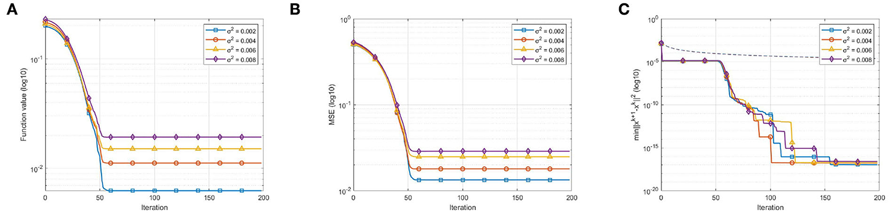
Figure 1. Convergence behavior in the case of noisy data: (A) Function value vs. number of iterations, demonstrates the sufficient desent and convergent property of the function value sequence {f(x^k)}; (B) MSE vs. number of iterations, demonstrates the convergent property of the point sequence {x^k}; (C) $\underset{0\le k\le n}{min}||x^{k+1}-x^k|{|}^2$ vs. number of iterations, where the dotted lines indicate the right side of Equation (14), verifies the bound of convergent rate.

The second experiment examines the convergence behavior of the ModelBI algorithm for Model B. The initialization step is obtained by applying 50 iterations of the power method in Candès et al. [27, Algorithm 3] to ensure the assumption ||x⁰ − x|| ≤ 1 in Proposition 5.2 with high probability. The constant for the MAP is set to $L=\frac{2}{m}{\sum }_{i=1}^m\left(b_i+\frac{1}{4}||a_i|{|}^2\right)||a_i|{|}^2$ due to Proposition 5.2. We stop after 2000 iterations in each trial and report the convergence results in Figure 2. As is shown in Figure 2, the sequence {x^k} generated by ModelBI results in a sufficient desent sequence {f(x^k)} and a critical point x* with the convergent rate bound in Equation (14).

FIGURE 2

Figure 2. Convergence behavior in the case of noisy data: (A) Function value vs. number of iterations, demonstrates the sufficient descent and convergent property of the function value sequence {f(x^k)}; (B) MSE vs. number of iterations, demonstrates the convergent property of the point sequence {x^k}; (C) $\underset{0\le k\le n}{min}||x^{k+1}-x^k|{|}^2$ vs. number of iterations, where the dotted lines indicate the right side of Equation (14), verifies the bound of convergent rate.

Remark 7. In Figure 1C, we observe that the curves are piecewise descending. This convergence behavior is due to the structure of the model function. The model function (16) constructed for Model A is still nonsmooth. As mentioned in Section 3, we picked a specific element ξ^k+1 from the set ${\partial }_{x}f(x^{k+1};x^k)$ at random in the first experiment. This strategy manifests itself as the piecewise decending curves in Figure 1C.

Remark 8. In Figure 2B, the MSE curves descend at first and slightly rise later. We observe that the ModelBI using a smooth model function makes the sequence {x^k} rapidly converge to the true solution in early iterates. Afterward, the sequence gradually converges into a noisy solution. The rising range is determined by the noise level σ. As Figure 2B shows, after about 400 iterates, the MSE curve with σ² = 0.002 rises less than that with σ² = 0.008. A proper stopping criterion can output a better result, but that is not what the manuscript mainly concerned about.

The third experiment presents the special behavior of iterative regularization by comparing our algorithm with the recently reported Model BPG algorithm [10]. The settings are respectively the same as that used in the experiments above. We do not have explicit solutions for Model BPG with these settings. For comparative purposes, we also apply ADMM with single-step iteration to the main computational step of Model BPG. For Model A, we stop after 200 iterations in each trial and report the convergence behaviors with σ² = 0.004 in Figure 3A. For Model B, we stop after 2,000 iterations in each trial and report the convergence behaviors with σ² = 0.004 in Figure 3B.

FIGURE 3

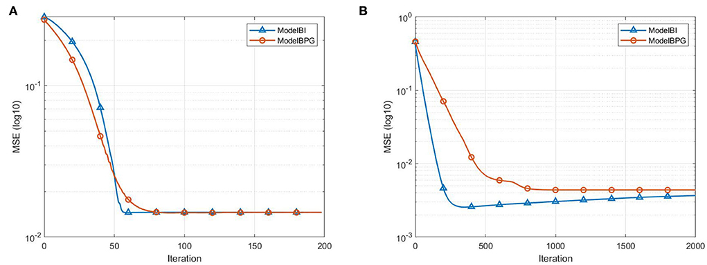
Figure 3. Convergence behavior in the case of noisy data with σ² = 0.004: (A) MSE vs. number of iterations, presents the convergence behavior of ModelBI and Model BPG for Model A; (B) MSE vs. number of iterations, presents the convergence behavior of ModelBI and Model BPG for Model B.

7. Conclusion

Bregman iterative regularization and its variants have attracted widespread attention in solving nonconvex problems, while it is still difficult in extending to generic nonsmooth composite optimization. In this regard, we proposed the ModelBI algorithm that is applicable to nonconvex nonsmooth problems based on the recent developments of the LBI and the model function. By taking advantage of the MAP, we drive the global convergence analysis of the ModelBI sequence. Moreover, we present the application of two kinds of nonsmooth phase retrieval problems by designing their model functions and iterative schemes. The application demonstrates the power of ModelBI, which appears to be the first Bregman iterative regularization method for solving these two kinds of problems.

Data availability statement

The original contributions presented in the study are included in the article/supplementary material, further inquiries can be directed to the corresponding author.

Author contributions

HZ and HY conceived of the presented idea. HY developed the theory and performed the computations. HW and LC verified the analytical methods. HW encouraged HY to investigate nonconvex phase retrieval model and supervised the findings of this work. All authors discussed the results and contributed to the final manuscript.

Funding

This study was supported in part by the National Natural Science Foundation of China (Nos. 11971480 and 61977065) and the 173 Program of China (No. 2020-JCJQ-ZD-029).

Acknowledgments

The authors would like to thank the referees and the associate editor for valuable suggestions and comments, which allowed us to improve the original presentation.

Conflict of interest

The authors declare that the research was conducted in the absence of any commercial or financial relationships that could be construed as a potential conflict of interest.

Publisher's note

All claims expressed in this article are solely those of the authors and do not necessarily represent those of their affiliated organizations, or those of the publisher, the editors and the reviewers. Any product that may be evaluated in this article, or claim that may be made by its manufacturer, is not guaranteed or endorsed by the publisher.

References

1. Osher S, Burger M, Goldfarb D, Xu J, Yin W. An iterative regularization method for total variation-based image restoration. SIAM J Multiscale Model Simulat. (2005) 4:460–89. doi: 10.1137/040605412

PubMed Abstract | CrossRef Full Text | Google Scholar

2. Yin W, Osher S, Goldfarb D, Darbon J. Bregman iterative algorithms for ℓ₁-minimization with applications to compressed sensing. SIAM J Imaging Sci. (2008) 1:143–68. doi: 10.1137/070703983

CrossRef Full Text | Google Scholar

3. Lorenz DA, Schöpfer F, Wenger S. The linearized bregman method via split feasibility problems: analysis and generalizations. SIAM J Imaging Sci. (2014) 7:1237–62. doi: 10.1137/130936269

CrossRef Full Text | Google Scholar

4. Lai MJ, Yin W. Augmented ℓ₁ and nuclear-norm models with a globally linearly convergent algorithm. SIAM J Imaging Sci. (2013) 6:1059–91. doi: 10.1137/120863290

CrossRef Full Text | Google Scholar

5. Zhang H, Yin W. Gradient methods for convex minimization: better rates under weaker conditions. CAM Report 13-17, UCLA (2013).

Google Scholar

6. Benning M, Betcke MM, Ehrhardt MJ, Schönlieb CB. Choose your path wisely: gradient descent in a Bregman distance framework. SIAM J Imaging Sci. (2021) 14:814–43. doi: 10.1137/20M1357500

CrossRef Full Text | Google Scholar

7. Zhang H, Zhang L, Yang HX. Revisiting linearized bregman iterations under lipschitz-like convexity condition. arXiv:2203.02109. (2022) doi: 10.1090/mcom/3792

CrossRef Full Text | Google Scholar

8. Drusvyatskiy D, Ioffe AD, Lewis AS. Nonsmooth optimization using Taylor-like models: error bounds, convergence, and termination criteria. Math Program. (2021) 185:357–83. doi: 10.1007/s10107-019-01432-w

CrossRef Full Text | Google Scholar

9. Ochs P, Fadili J, Brox T. Non-smooth non-convex bregman minimization: unification and new algorithms. J Optim Theory Appl. (2019) 181:244–78. doi: 10.1007/s10957-018-01452-0

CrossRef Full Text | Google Scholar

10. Mukkamala MC, Fadili J, Ochs P. Global convergence of model function based Bregman proximal minimization algorithms. J Glob Optim. (2021) 83:753–81. doi: 10.1007/s10898-021-01114-y

CrossRef Full Text | Google Scholar

11. Rockafellar RT. Convex Analysis. Princeton, NJ: Princeton University Press (1970).

Google Scholar

12. Bregman LM. The relaxation method of finding the common point of convex sets and its application to the solution of problems in convex programming. Ussr Comput Math Math Phys. (1967) 7:200–17. doi: 10.1016/0041-5553(67)90040-7

CrossRef Full Text | Google Scholar

13. Bauschke HH, Borwein JM. Legendre functions and the method of random bregman projections. J Convex Anal. (1997) 4:27–67.

14. Kiwiel KC. Proximal minimization methods with generalized Bregman functions. SIAM J Control Optim. (1997) 35:1142–68. doi: 10.1137/S0363012995281742

CrossRef Full Text | Google Scholar

15. Kiwiel KC. Free-Steering relaxation methods for problems with strictly convex costs and linear constraints. Math Oper Res. (1997) 22:326–49. doi: 10.1287/moor.22.2.326

CrossRef Full Text | Google Scholar

16. Chen G, Teboulle M. Convergence analysis of a proximal-like minimization algorithm using Bregman functions. SIAM J Optim. (1993) 3:538–43. doi: 10.1137/0803026

CrossRef Full Text | Google Scholar

17. Bauschke HH, Bolte J, Teboulle M. A descent lemma beyond Lipschitz gradient continuity: first-order methods revisited and applications. Math Operat Res. (2017) 42:330–48. doi: 10.1287/moor.2016.0817

CrossRef Full Text | Google Scholar

18. Bolte J, Sabach S, Teboulle M. Proximal alternating linearized minimization for nonconvex and nonsmooth problems. Math Program. (2014) 146:459–94. doi: 10.1007/s10107-013-0701-9

PubMed Abstract | CrossRef Full Text | Google Scholar

19. Bolte J, Daniilidis A, Lewis A. The Łojasiewicz inequality for nonsmooth subanalytic functions with applications to subgradient dynamical systems. SIAM J Optim. (2007) 17:1205–23. doi: 10.1137/050644641

CrossRef Full Text | Google Scholar

20. Bolte J, Daniilidis A, Lewis A, Shiota M. Clarke subgradients of stratifiable functions. SIAM J Optim. (2007) 18:556–72. doi: 10.1137/060670080

CrossRef Full Text | Google Scholar

21. Beck A. First-Order Methods in Optimization. SIAM-Soc Ind Appl Math. (2017) doi: 10.1137/1.9781611974997

CrossRef Full Text | Google Scholar

22. Rubin W. Principles of Mathematical Analysis. 3rd ed. New York, NY: McGraw-Hill (1976).

Google Scholar

23. Dong J, Valzania L, Maillard A, an Pham T, Gigan S, Unser M. Phase retrieval: from computational imaging to machine learning. arXiv:2204.03554. (2022). doi: 10.48550/arXiv.2204.03554

CrossRef Full Text | Google Scholar

24. Hilal A, Duchi JC. The importance of better models in stochastic optimization. Proc Natl Acad Sci USA. (2019) 116:22924–30. doi: 10.1073/pnas.1908018116

PubMed Abstract | CrossRef Full Text | Google Scholar

25. Pinilla S, Bacca J, Arguello H. Phase retrieval algorithm via nonconvex minimization using a smoothing function. IEEE Trans Signal Process. (2018) 66:4574–84. doi: 10.1109/TSP.2018.2855667

CrossRef Full Text | Google Scholar

26. Ouyang Y, Chen Y, Lan G, Pasiliao E. An accelerated linearized alternating direction method of multipliers. SIAM J Imaging Sci. (2015) 8:644–81. doi: 10.1137/14095697X

PubMed Abstract | CrossRef Full Text | Google Scholar

27. Candès EJ, Li X, Soltanolkotabi M. Phase retrieval via wirtinger flow: theory and algorithms. IEEE Trans Inf Theory. (2015) 61:1985–2007. doi: 10.1109/TIT.2015.2399924

CrossRef Full Text | Google Scholar