 Yongsheng Chen
 Jue Yan
 Xinghui Zhong
- 1School of Mathematical Sciences, Zhejiang University, Hangzhou, China
- 2Department of Mathematics, Iowa State University, Ames, IA, United States
In this paper, we develop the cell-average based neural network (CANN) method to solve third order and fifth order Korteweg-de Vries (KdV) type equations. The CANN method is based on the weak or integral formulation of the partial differential equations. A simple feedforward network is forced to learn the cell average difference between two consecutive time steps. One solution trajectory corresponding to a generic initial value is used to generate the data set to train the network parameters, which uniquely determine a one-step explicit finite volume based network method. Once well-trained, the CANN method can be generalized to a suitable family of initial value problems. Comparing with conventional explicit methods, where the time step size is restricted as Δt = O(Δx3) or Δt = O(Δx5), the CANN method is able to evolve the solution forward accurately with a much larger time step size of Δt = O(Δx). A large group of numerical tests are carried out to verify the effectiveness, stability and accuracy of the CANN method. Wave propagation is well resolved with indistinguishable dispersion and dissipation errors. The CANN approximations agree well with the exact solution for long time simulation.
1. Introduction
In this paper, we develop the cell-averaged based neural network (CANN) method [1] for four classes of nonlinear wave equations formulated by the third order Korteweg-de Vries (KdV) equations
the fully nonlinear K(m, n) equations
the KdV-Burgers type equations
and the fifth order KdV type equations
where ϵ is a constant and ξ(u) ≥ 0, f(·), r(·), g(·), s(·), and h(·) are arbitrary (smooth) nonlinear functions.
The KdV equations (1.1), introduced in [2] a century ago as a model for small amplitude long wave motion on the surface of shallow water waves, are one of the basic models of soliton theory. The fully nonlinear K(m, n) equations (1.2) are useful for describing the dynamics of various physical systems, and admit compactly supported solitary waves solutions, i.e., the so-called compacton solution [3]. The KdV-Burgers equation (1.3) arises in the description of long wave propagation in shallow water and in weakly nonlinear plasma physics with dissipation [3]. The fifth order nonlinear KdV equation (1.4) arises in the modeling of weakly nonlinear waves in a wide variety of media including magneto-acoustic waves in plasma and long waves in the liquids under ice sheets [4, 5]. These KdV type equations describe nonlinear wave motion that incorporate several important physical phenomena, namely, dispersion, nonlinear advection, and viscosity, and are commonly found in applications such as nonlinear optics, Bose-Einstein condensation, plasma physics, biophysics, etc.. Various conventional numerical methods were carried out to solve these KdV type equations; see [6–10] and the references therein.
Over the last three decades, machine learning with neural networks has achieved tremendous success in image classification, speech recognition, text and natural language processing, etc.. In the last few years, extensive studies with neural network appear in scientific computing, now referred as the field of scientific machine learning. Early works include the integration of ODE or PDE to networks in [11, 12], discovery of PDEs in [13, 14], solving high-dimensional PDEs in [15–17], and applications for uncertainty quantification in [18–24], etc.. Another popular direction combines neural network with classical numerical methods to improve their performance, for example, as troubled-cell indicator in [25], to estimate the weights and enhance WENO scheme in [26], convolution neural networks (CNN) for shock detection for WENO schemes in [27], and to estimate the total variation bounded constant for limiters in [28].
Recently, neural network has been applied to directly solve ODEs and PDEs, among which they can be roughly classified into two approaches. The first approach parameterizes the solution as a neural network or a deep CNN between finite Euclidean spaces. Approximation properties of neural networks are explored in [29–31] and the method is mesh free and enjoys the advantage of auto differentiation. There have been early works in [32–37] and the popular PINN method in [38–43]. We skip the long list. While PINN methods are successful for elliptic type PDEs, the method is inefficient for time evolution problems due to its approximation is limited to a fixed time window.
The second group of methods, the so-called neural operator approach, produce a single set of network parameters that may be used in discretizations. It needs to be trained only once and a solution for a new instance of parameter requires only a forward pass of the network. Works in this approach include the graph kernel neural network [44] and the Fourier neural operator [45], which learn the mapping between infinite-dimensional spaces and most closely resembles the reduced basis method. The cell-average based neural network (CANN) method discussed in this paper explores a simple network that approximates the cell average difference between two consecutive time steps, which can be considered as operator approximation and be classified into this approach. The CANN method was first developed in [1] for hyperbolic and parabolic equations, motivated by the work of [46] that also explored the approximation of the solution difference between two time instances. The CANN method we aim to develop for KdV type equations essentially defines a forward in time evolution mechanism, which can be applied to propagate the wave solution in time as a regular explicit method. We also refer readers to the early work of cellular nonlinear network for KdV equation [47].
The CANN method combines the neural network with the finite volume scheme, where a shallow feedforward network is explored to learn the cell average difference between two consecutive time steps. After well trained, an explicit one-step finite volume type neural network method is obtained. A major advantage of the CANN method is that the neural network solver can be relieved from the Courant-Friedrichs-Lewy (CFL) restriction of explicit schemes and can adopt large time step size (i.e., Δt = 4Δx). In this paper, we continue to develop the CANN method for KdV type equations (1.1–1.4), which are third order or fifth order nonlinear equations with dispersive feature. The CANN method is further developed to solve these high order equations with large time step size (i.e., Δt = Δx/2), which can be considered as an explicit time discretiztaion method efficiently propagating the dispersive wave evolution forward in time.
The starting point of CANN method is the weak formulation of the time dependent problem (1.1–1.4) obtained by integrating the equation over the box of spatial cell and temporal interval. With the notation of cell averages, the rewritten integral form of the equation can be regarded as the cell average difference between two consecutive time levels, for example, between tk and tk+1. The CANN method applies a simple network to approximate the cell average difference between such two time levels. One important feature is the introduction of the network input vector, which can be interpreted as the stencil of the scheme at time level tk. The major contribution of the CANN method is to explore such a network structure that exactly matches an explicit one-step finite volume scheme. Thus the network parameter set, after offline supervised learning from a given data set, behaves as the coefficients of the scheme. After well trained, the CANN method is a local and mesh dependent solver that can be applied to solve the equation as a regular explicit method.
Essentially the CANN method can be considered as a time discretization scheme, for which it is critical to maintain the stability and control the accumulated error in time. Numerical tests show that it is necessary to include multiple time levels of data to train the network and obtain a stable CANN solver. In the original CANN method [1], multiple time levels of data pairs are used and treated equally over the training process, which does not take into account the accumulation error. In this paper, we modify the training procedure by connecting all time levels of data and by forcing the accumulation error to roll over to the next time level such that a stable CANN method can be obtained.
In this paper, we pick one generic initial value u(x, 0) = u0(x) of the given PDE (1.1–1.4) to generate the training data set. In a word, cell averages from a single solution trajectory are used to train the network. It turns out that the CANN method is able to learn the mechanism of nonlinear dispersive wave propagation with such a small training data set (up to t5 five time steps). Once well trained, the CANN solver can be applied to solve a group of initial values problems of (1.1–1.4) with insignificant generalization error. Numerical tests show a shallow network [48] in terms of two or three hidden layers and a total of a few hundred unknowns of weights and biases is sufficient for obtaining a well-behaved CANN method. Comparing with conventional explicit methods, where the time step size is restricted as Δt = O(Δx)3 or Δt = O(Δx)5, the CANN method can accurately maintain the evolution of the solution in time with a much larger time step size as Δt = O(Δx). Numerical tests for four classes of the KdV equations are carried out to verify the stability, accuracy, and effectiveness of the CANN method.
The rest of the paper is organized as follows: In Section 2, we present the details of the CANN method for solving the KdV type equations with the problem setup and formulation of the CANN method in Section 2.1, data generation and the training process in Section 2.2, and implementation and discussion of the CANN method in Section 2.3. Various numerical experiments are shown in Section 3. Conclusion remarks are given in Section 4.
2. Cell-average based neural network approximation
2.1. Problem setup and the CANN method
The CANN method is closely related to the finite volume scheme, which is a mesh-dependent local solver. Similar to the finite volume method, we start with mesh partition in space and time. The computational domain [a, b] is uniformly partitioned into J cells with , where
The cell size is denoted as . The time domain is also uniformly partitioned with time step size Δt, and the k-th time level is denoted as tk = kΔt.
To derive the CANN method, we first rewrite the KdV type equations (1.1–1.4) in the following form
where is the differential operator that includes all terms involving spatial variable x. Integrating (2.1) over a generic computational cell Ij and time interval [tk, tk+1] yields
Let denote the cell average of the solution on Ij. Equation (2.2) can be integrated out as
Clearly, exact solutions of the KdV type equations satisfy (2.3) with being the associated differential operator. Equation (2.3) is a weak formulation and is equivalent to the associated KdV type equation (1.1–1.4) under suitable regularity.
The integral form of (2.3) is the starting point for designing the CANN method. Instead of applying numerical differentiation to the complicated operator , a fully connected feedforward neural network is sought to approximate the right hand side of (2.3), namely,
We assume such a mapping exists, represented through a network , where is the network input vector. We highlight that the input vector involve the solution information at time level tk and cell Ij and is the window to communicate with the network. All network parameters of weight matrices and biases are grouped into and denoted by Θ. Suppose that the training data pair involving the cell averages at time level tk and tk+1 are available, a simple network is trained to minimize the square error between the network output and the given data , where
Setting and connecting (2.5) with (2.3), the goal of the CANN method is to enforce the network output to approximate the cell average at next time level tk+1, i.e.,
We refer to Figure 1 for the structure of the CANN method. From the format of (2.5), we see our network is a variation of residual neural network method. The input of our network is a vector while the output is a scalar. The leading entry of the input vector is used to compute the residual. The network is trained to learn the residual or the solution evolution from tk to tk+1.
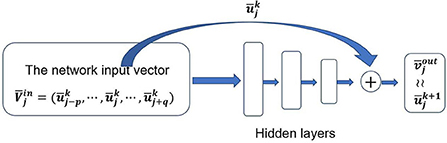
Figure 1. Network structure of a CANN method.
In a word, a shallow network is pursued to approximate the cell average difference between two consecutive time levels. The input vector of the network (2.5) is given by
which includes p left cell averages and q right cell averages of . The functionality of the input vector is similar to the stencil of a conventional numerical method. The components of the input vector, i.e., the values of p and q, determine the effectiveness of the CANN method and thus need to be carefully chosen. The general principle is to follow the PDE and the characteristic of the solution to design a suitable network input vector. For a dispersive differential equation with wave propagating from right to left, i.e., ut + uxxx = 0, more cells to the right (q > p) should be included in the network input vector (2.6) to adapt the dispersive relation.
The network parameter set Θ can be considered as the scheme coefficients of a finite volume type neural network method. The so-called optimal network parameter set Θ* is obtained through offline supervised learning with data distributed over all spatial cells Ij, j = 1, …, J. The well-trained neural network essentially behaves as an explicit one-step finite volume scheme, which is supposed to solve general initial value problem of the KdV type equations (1.1–1.4) at any time level tk and on any cell Ij.
The network structure of the CANN method is illustrated in Figure 1. We consider a standard fully-connected neural network with M (M ≥ 3) layers. The first layer is the input vector of (2.6) which is the stencil with p cells to the left and q cells to the right of the current cell Ij. The last layer is the cell average approximation at next time level tk+1. The M − 2 layers in the middle are hidden layers. Let ni denote the number of neurons in the i-th layer. We have n1 = p + q + 1 and nM = 1. The abstract objective of machine learning is to find a mapping such that, is able to accurately approximate , the right hand side of (2.3).
The network is a composition of the following operators
where ⚬ represents the composition operator, and Wi denotes the linear transformation operator or the weight matrix connecting the neurons from the i-th layer to the (i + 1)-th layer. Activation functions σi:R → R(i ≥ 2) are applied to each neuron in a component-wise fashion. In this paper, we adopt σi(x) = tanh(x) for i = 2, …, M − 1 and σM(x) = x.
Definition 1. The CANN method is well-defined by the following three components: (1) the spatial and temporal mesh sizes Δx and Δt; (2) the network input vector defined in (2.6); (3) the structure of the neural network in terms of number of hidden layers and neurons per layer.
In this paper, we explore one generic initial value of the given PDE (1.1–1.4) to generate the training data set. In a word, a single solution trajectory is considered and used to train the network. To maintain the stability and control the accumulation error in time, multiple time levels of cell averages are needed and included in training. It turns out that the CANN method is able to learn the mechanism of nonlinear dispersive wave propagation with such a small training data set. Once well trained, the CANN solver can be applied to solve a group of initial values problems of (1.1–1.4) with insignificant generalization error. We further highlight that numerical tests show a shallow network in terms of two or three hidden layers and a total of a few hundred unknowns of weights and biases is sufficient for obtaining a well-behaved CANN method (2.5).
2.2. Data generation and training of the CANN method
In this section, we present the generation of the data set and the training process of the CANN method, which are important steps toward the success of the CANN method.
The training data set is taken as one generic initial value problem with u(x, 0) = u0(x), and one single solution trajectory is explored to generate cell averages as the learning data. The training data set is defined by
which consists of one trajectory of cell averages spreading over the whole computational domain (j = 1, …, J) and covering time levels from t0 to tn. The cell averages are either generated from the exact solution or obtained from a highly accurate numerical method corresponding to the picked initial value problem.
The geometric structure of the data set S can be regarded as rectangular shape with the horizontal direction representing spatial cells with index j = 1, …, J and the vertical direction representing time levels with index k = 0, …, n. It is worth mentioning that there is no analytical result about how many time levels should be included in the data set to obtain a stable CANN method. In this paper, numerical experiments show that time levels up to t5 [n = 5 in (2.8)] are good enough for training the network such that a stable CANN method can be obtained for all four classes of the KdV type equations.
Now we discuss in detail the supervised learning process with the data of (2.8) to obtain the optimal parameter set Θ*, which is the goal of the CANN method such that the network can accurately approximate the operator or the difference between two consecutive time levels. As discussed in Section 2.1, the network parameter set Θ behaves more or less as the coefficients of a finite volume scheme. The CANN method (2.5), after well trained, is an explicit one-step method that will be applied on any cell Ij and at any time level tk. Thus the network parameter set Θ should be updated independent of the data location (j, k) and should be continuously updated while the cell index looping through the spatial domain (j = 1, …, J).
In the original CANN method [1], the training data is used in the form of pairs . The parameter set Θ is updated with applied forming the input vector , while the square error or the loss function
is minimized through the network (2.5). Even for nonlinear problems with multiple time levels of data on hand, different time levels are used and treated equally in [1]. Since the parameter set Θ is essentially the coefficients of a one-step method, it is reasonable to apply the data usage in this way and enforce the network learning the evolution of . On the other hand, this training procedure does not take into account the error accumulated in time. It is worth emphasizing that such a process of training is not stable for nonlinear KdV type equation involving advection, diffusion, and dispersion terms.
To maintain the stability and control the accumulation errors in time, we connect all time levels of data in the training set (2.8) and modify the data usage and training process. We force the accumulation error roll over to the next time level during training such that the accumulation error is part of the training procedure itself. Except the first two time levels t0 and t1, we follow the original CANN method and apply data pairs of to update parameter set Θ. For any later two consecutive time levels tk and tk+1 (1 ≤ k ≤ n − 1), data pairs of are adopted in the network (2.5) to update the parameter set Θ. Here the network outputs at tk, which are obtained through the network (2.5) with the updated Θ, are used to assemble the network input vector , instead of using as the original CANN method. It is worth mentioning that . The network input vector inherits the accumulation error from previous time levels and will flow this information into the CANN network to update . We then minimize the square error of with a optimization method, for example, the stochastic gradient descent to update Θ for the next round. We refer to Figure 2 for the illustration of data usage and the modified training process for Θ.
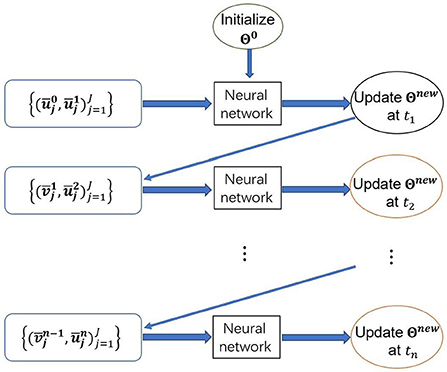
Figure 2. Illustration of data usage and one epoch iteration to update Θ.
To speed up training and improve accuracy, we apply the mini-batch stochastic gradient descent method with the batch size set as jb = 10. The loss function is defined as
where 1 ≤ jm1, …, jmjb ≤ J are the total jb randomly selected indices for each batch m = 1, …, J/jb. Following [49], Adam optimization algorithm is applied to train the parameters Θ. Initial learning rate of α = 0.01 or α = 0.001 is adopted and later attenuated learning rate is applied through Adam method.
All matrices weights are first randomly generated from a normal distribution around zero. The biases are initialized to be zero. One epoch of iteration is defined as the network parameters Θ being continuously updated with each piece of data in the set of (2.8) applied once.
The parameter set Θ will be updated corresponding to the coverage order of the data set. We first sweep through spatial cells over the whole computational domain, then move toward temporal direction to accommodate more time levels of data to improve the stability of the method. Specifically, one epoch of iteration is corresponding to the procedure described from line #7 to line #19 in the pseudo code of Algorithm 1. The parameter set Θ is to be continuously updated through the mini-batch gradient descent direction of (2.9). For one epoch iteration, the parameter set Θ is updated with a total of n × (J/jb) times. It is worth mentioning that following squared L2 error at the last time level tn
is calculated and used as the objective and the measurement of the effectiveness of the CANN method (2.5). We refer to Algorithm 1 as a flow chart of the training procedure for the CANN method.
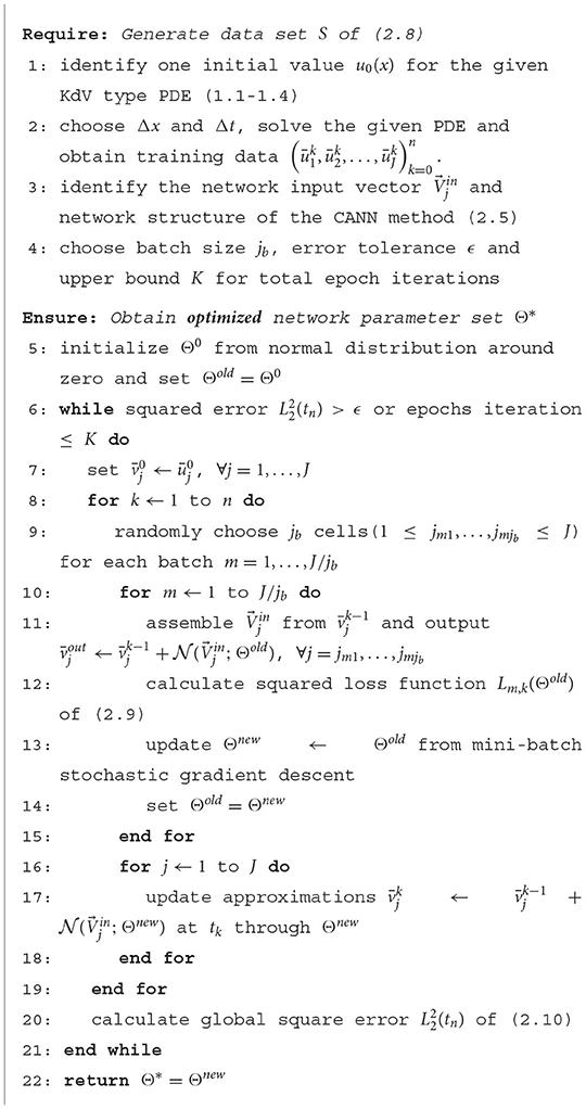
Algorithm 1. Training of the network parameter Θ* for the CANN method.
We mention again that multiple time levels of data are necessary to train a stable CANN method for nonlinear KdV type equations. With the new way of data application, the accumulation error in time is considered over the training process, which undoubtedly improves the stability of the CANN method. The data set S of (2.8) involving multiple time levels of data can be regarded as a one identity or one body of the training data.
We further highlight that the term optimal is an abused notation. We assume that the network mapping exists and well approximates the right hand side of (2.3) with small error (). The parameter set Θ* does not refer to the set corresponding to the minimizer of (2.9). Instead, the term of the optimal parameter set Θ* refers to any collection of network weights and biases that can manage the squared error (2.10) smaller than a given tolerance.
Notice for j = 1 or j = J or those close to boundary cells, the network input vector in (2.6) requires p left cells and q right cells to update the current cell during both training and implementation. This is similar to the boundary condition scenario of a conventional finite volume method. In this paper, we restrict our attention on Dirichlet or periodic boundary conditions. During training and implementation, we simply copy cell averages from inside the domain to accommodate periodic boundary conditions.
2.3. Implementation and discussion of the CANN method
It follows from the discussion in previous sections that, with the spatial and temporal mesh sizes Δx and Δt chosen, the network input vector picked, and the optimal network parameter Θ* successfully trained, the CANN method is well defined. Now, with available, the trained CANN method can be implemented as an explicit one-step time discretization method as follows: starting from cell averages of a solution at time level tk (for the initial condition, is taken as the cell averages of the given initial condition), we would like to advance it to next time level tk+1 to obtain by
Implementation of the CANN method
1 Compute the initial cell averages at t0 from the given initial condition.
2 Run through the CANN method (2.11) to generate cell average approximations for later time.
3 Repeat Step 2 until the expected time is reached.
Periodic or Dirichlet type boundary conditions are implemented in the same way as a conventional finite volume method. It is worth mentioning again that the CANN method trained with the data generated from one generic initial condition of the given problem (1.1–(1.4 can be applied to a suitable family of initial value equations.
One typical phenomena observed is that the CANN method as an explicit method can be relieved from the stringent CFL restriction on time step size. For third order dispersive equations, i.e., ut + uxxx = 0, conventional explicit methods require the time step size to be as small as Δt ≈ O(Δx)3. For fifth order equations, i.e., ut − uxxxxx = 0, the restriction is more stringent with Δt ≈ O(Δx)5. Instability and blowup phenomena will be observed if a larger time step size is applied. Explicit methods are limited by the small time step size, thus are time consuming and inefficient especially for multi-dimensional problems. Many efforts are made to investigate implicit or semi-implicit time discretization methods. Implicit methods have the advantage of large time step size, though the algorithms are usually complicated and sometimes are also expensive.
It is worth emphasizing that the neural network method is based on the integral format of the PDE
It is equivalent to the original PDE, i.e., , given in differentiation form. Due to unknown reason behind, the CANN method is able to catch up solution information at the next time level tk+1 and adapt large time step size for solution evolution, which is similar to an implicit method. Numerical tests show that the CANN method can adopt very large time step size as Δt = O(Δx) for KdV type equations involving third order or fifth order terms.
The following is a summary of the properties of the CANN method.
• The CANN method is based on the integral formulation of the PDE.
• Numerical tests show that CANN method can adopt very large time step size of Δt = O(Δx) for third order or fifth order KdV type equations.
• Small data set can be used to effectively train the network and obtain a stable and accurate explicit one-step finite volume type method.
• The CANN method can sharply evolve the compacton propagation with no oscillation at the singular corners and has no difficulty to capture solution with sharp transition.
• The CANN method generates little dispersive and dissipation errors for long time simulation.
The CANN method, trained from a single solution trajectory with a single wave speed, is able to solve a collection of wave propagation problems with different wave amplitudes and wave speeds. We end this section with some comments on the limitations associated with the current version of the method. In this paper, we explore extremely small-sized data set generated from one single solution trajectory corresponding to the chosen choice of wave speed and wave amplitude among the family of soliton wave solutions. In some cases, the CANN method is less accurate when tested on soliton solutions with the parameter such as the wave speed that is far away from the one used in training. Furthermore, the CANN method needs a rather wider or larger input vector , while conventional numerical method has more compact stencil for scheme definition.
3. Numerical results
In this section, we carry out a series of numerical experiments to demonstrate the accuracy and capability of the CANN method for the KdV type equations (1.1–1.4). The major objective is to verify that large time step size, i.e., Δt = Δx/8, can be applied to explicitly solve high order PDEs. One initial value is picked and one single solution trajectory is explored to generate the training data set (2.8). The well-trained network solver is able to solve a group of initial value problems with insignificant generation error.
We present simulations of the CANN method for the third order KdV equations in Section 3.1, for the fully nonlinear K(m, n) equation in Section 3.2, for the KdV-Burgers equations in Section 3.3, and for the fifth order KdV equations in Section 3.4. To show the performance of the CANN method, we examine the following two error measures.
• L2 error:,
• L∞ error: ,
where denotes the numerical solution obtained by the proposed CANN method and ūj(T) denotes the cell average of the exact solution. Here the final time T is always taken as a multiple of the time step since the time step Δt is chosen first and is a part of the CANN method (2.11).
3.1. Third order KdV equations
In this subsection, we present numerical results for the third order generalized KdV equations (1.1) with the CANN method (2.11).
Example 3.1. In this example, we consider the following classical KdV equation
with ϵ = 5 × 10⁻⁴. The computational domain is set as [0, 2], and periodic boundary conditions are applied. There exist classical soliton wave solutions [50] given by
where x0 is the wave center, c relates to the wave amplitude and speed, and κ is determined by c and by the dispersive coefficient ϵ via .
Now we explore the CANN method for the above soliton wave solutions of the KdV equation (3.1). We adopt the spatial mesh size Δx = 0.0125 and large time step size for setting up the CANN method. The network input vector
is considered since the wave propagates from left to right. The network structure consists of three hidden layers with 40, 20, and 10 neurons in the first, second, and third layers, respectively.
The training data set is generated from the solution of (3.2) with c = 0.3 and x0 = 0.5. A total of K = 2 × 10⁵ epoch iterations are applied to train the network. After well trained, the CANN network solver is applied to test on a group of soliton solutions (3.2) with various values of c and x0. For the first test, we fix the wave center location x0 = 0.5 in (3.2) and change the values of c relating to both wave speed and wave amplitude. Table 1 lists the L2 and L∞ errors between the CANN solution and the exact solution at T = 0.25 for different values of c. For the second test, we fix the wave speed/amplitude c = 0.3 in (3.2) and change the locations of the wave center x0. Figure 3 plots the simulations of the CANN method at T = 0.5 with different locations x0. It can be observed that the CANN method is able to accurately capture a decent collection of soliton waves (3.2) for the KdV equation (3.1).
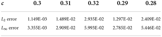
Table 1. Errors of the CANN simulation for Example 3.1 at T = 0.25 with different c.
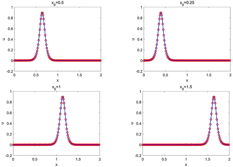
Figure 3. Soliton solutions (3.2) of Example 3.1: the CANN solution (red circles) and the exact solution (solid blue lines) at T = 0.5 with c = 0.3 for different values of x0.
Example 3.2. In this example, we consider the following generalized KdV equation
with ϵ = 0.2058 × 10⁻⁴ over the computational domain [−2, 3]. Zero boundary conditions are applied. Similar to (3.1), soliton wave solutions [7] exist and are given by
Here A is the wave amplitude, and x0 is the initial wave center. The wave frequency is determined by A and ϵ. The wave speed ω is given by .
Similar to previous example, we set the spatial mesh size as Δx = 0.0125 and the time step size as . A relatively narrower network input vector
is adopted, and only one hidden layer of 40 neurons is taken for the network structure.
The training data set is generated from the soliton solution of (3.5) with A = 0.2275 and x0 = 0.5. A total of K = 2 × 10⁵ epochs are applied for training the network. Once well trained, the network solver is applied to test on a group of soliton solutions (3.5) with different values of A and x0. We show the L2 and L∞ errors between the CANN simulation and the exact solution at T = 1 in Table 2. The left column lists the errors with the location x0 = 0.5 fixed but with different values of A in (3.5), while the right column lists the errors with A = 0.2275 fixed but with different locations x0. For the group of soliton solutions (3.5) with various values of A or x0, the CANN approximations agree well with the exact solutions.
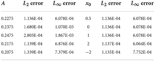
Table 2. Errors of the CANN solution for Example 3.2 at T = 1 with different A or x0.
3.2. Fully nonlinear K(m, n) equation
In this subsection, numerical tests with the CANN method for the fully nonlinear K(m, n) equations (1.2) are presented, where solutions with singular corners are typical, that are referred as compacton solutions; see e.g., [51, 52] for more details.
Example 3.3. In this example, we consider the following K(2, 2) equation
over the domain −20 ≤ x ≤ 20 and with periodic boundary conditions. We study the CANN method to the canonical traveling wave solutions of
given in [51], where the parameter λ determines both the wave speed and the wave amplitude.
For the CANN method, the spatial mesh size Δx = 0.1 and the temporal mesh size are taken. The network structure consists of two hidden layers with 40 and 20 neurons in the first and second layers, respectively. Due to the fact that the wave propagates from the left to right, the following neural network input vector is chosen
The training data set is generated from the compacton solution of (3.8) with λ = 1. A total of K = 2 × 10⁵ epochs are used to train the network. After well trained, the network solver is applied to simulate the evolution of the compacton (3.8) with different λ values. Figure 4 plots the CANN solutions at T = 0.5 with different λ. The CANN method trained from λ = 1 can be generalized to the compactons (3.8) with different values of λ not far away from 1.
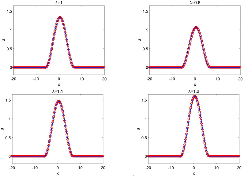
Figure 4. K(2, 2) equation in Example 3.3: the CANN solution (red circles) and the exact solution (solid blue lines) at T = 0.5 with different λ.
3.3. The KdV-Burgers equations
In this subsection, we present numerical results for the compound KdV-Burgers equation (1.3) in the form of
where α, μ, β, and ϵ are the constants to balance the convection, diffusion, and dispersive effects. These equations can be considered as a composition of the KdV and Burgers equations. We refer to [3] for more details of the equations and to [53] for the explicit form of exact solutions in (3.10).
Example 3.4. In this example, we consider the KdV-Burgers equation
over the computational domain −20 ≤ x ≤ 20 with α = 1, ϵ = 1, and β = −2. We study a group of traveling waves given by
where c and ω are determined by and with b and θ being arbitrary constants. Exact solutions at the boundaries are applied.
For the simulation, we choose Δx = 0.0125 and . The network contains two hidden layers with 40 neurons in the first layer and 20 neurons in the second layer. The network input vector is taken as
The training data set is generated from the wave solution (3.12) with b = 0 and θ = 0. A total of K = 1 × 10⁵ epochs are applied to train the network. After well-trained, the network solver is applied to solve wave solutions (3.12) with various values of b and θ. We first fix b = 0 in (3.12 and change the values of θ and plot the CANN simulations in Figure 5. We then fix θ = 0 and change the values of b, and plot the CANN simulations in Figure 6. It can be observed that the CANN method can be well-generalized to a family of wave solutions in the form of (3.12).
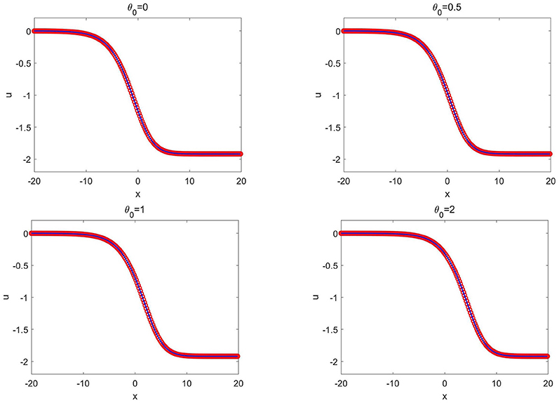
Figure 5. KdV-Burgers equation of Example 3.4: the CANN solution (red circles) and the exact solution (solid blue lines) at T = 1.0 with different θ.
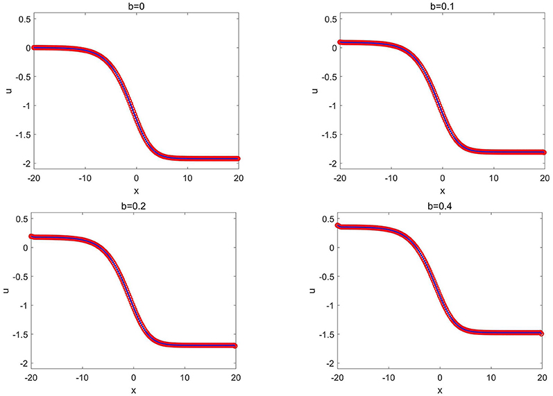
Figure 6. KdV-Burgers equation of Example 3.4: the CANN solution (red circles) and the exact solution (solid blue lines) at T = 1.0 with different b.
Example 3.5. In this example, we consider the mKdV-Burgers equation
with μ = 1.5, β = −1 × 10⁻⁴, and ϵ = 1. The computational domain is taken as −10 ≤ x ≤ 10. We study the following group of traveling wave solutions
where and ω = ϵ3 − βc2 − μa2b2c with a > 0, b, and θ being arbitrary constants. Exact solutions are applied as the given Dirichlet boundary condition for the CANN method.
The mesh sizes Δx = 0.0125 and are used to set up the CANN method. We adopt the following network input vector
The network structure is composed of three hidden layers with 40, 20, and 10 neurons in the first, second, and third layers, respectively. The training data set is generated from the solution of (3.14) with a = 1, b = 1, and θ = 0. A total of K = 2 × 10⁵ epochs are applied for training the network. After well trained, the network solver is applied to solve a group of wave solutions (3.14) with various values of a, b, and θ. Figure 7 shows the simulation of the CANN method with different values of a, b, and θ. We observe that the network solver can approximate the mKdV-Burgers equation well. The CANN method can be generalized to a large class of wave solutions in (3.14).
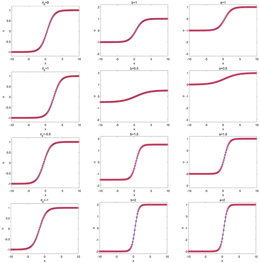
Figure 7. mKdV-Burgers equation of Example 3.5: the CANN solution (red circles) and the exact solution (solid blue lines) at T = 1.0. (Left) Different values of θ with a = 1 and b = 1; (Middle) Different values of b with a = 1 and θ = 0; (Right) Different values of a with b = 1 and θ = 0.
3.4. Fifth order KdV equations
In this section, we extend the study of the CANN method to the fifth order KdV equations (1.4).
Example 3.6. In this example, we consider the Kawahara equation
over the domain −20 ≤ x ≤ 20 with zero boundary conditions. We study the group of soliton wave solutions [5] given by
where the wave center x0 is an arbitrary constant.
To set up the CANN method, we take Δx = 0.0125 and and adopt the following network input vector
The structure of the network contains two hidden layers with 40 neurons in the first layer and 20 neurons in the second layer. The training data set is generated from the solution (3.17) with x0 = 0. A total of K = 2 × 10⁵ epochs are applied to train the network. Once well trained, the network solver is applied to solve a group of solutions (3.17) with different values of x0. Figure 8 presents the CANN simulations with x0 changing from −10 to 10. The CANN solutions match well with the exact solutions, and the CANN method can be applied to solve the group of wave solutions (3.17) with indistinguishable generalization error.
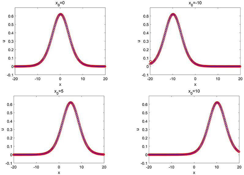
Figure 8. Kawahara equation of Example 3.6: the CANN solution (red circles) and the exact solution (solid blue lines) at T = 1.0 with different x0.
Moreover, we run the CANN solver for long time simulation to test the stability of the method. Figure 9 shows the CANN approximation to the solution (3.17) with x0 = 5 at T = 0, 10, 20, and 40. The method generates little numerical dissipation and dispersive error after long time simulation.
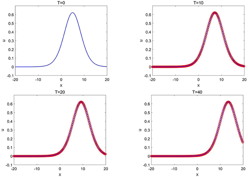
Figure 9. Kawahara equation of Example 3.6: the CANN solution (red circles) and the exact solution (solid blue lines) at different T with x0 = 5.
Example 3.7. In this example, we consider Ito's fifth order mKdV equation [4]
with α = −1. The computational domain is [−30, 30]. We consider to approximate the group of wave solutions in the form of
With the wave amplitude κ chosen, the wave speed is determined by ω = 6κ4. Here x0 is the wave center. Dirichlet boundary conditions from the exact solutions are applied.
For the CANN method, we set Δx = 0.0125 and choose . The network input vector
is adopted. The structure of the network consists of two hidden layers with 40 neurons in the first layer and 20 neurons in the second layer. The training data set is generated from the solution (3.20) with κ = 0.25 and x0 = −10. A total of K = 2 × 10⁵ epochs are applied for training the network.
Once well-trained, the network solver is applied to solve a group of wave solutions (3.20) with different values of κ and x0. We first fix κ = 0.25 and change the locations of x0, and show the CANN simulations in Figure 10. Figure 11 show the CANN simulations with the fixed location x0 = −10 but with different values of κ. The CANN method can be generalized to a family of wave solutions (3.20) over the range −10 ≤ x0 ≤ 20 and 0.25 ≤ κ ≤ 0.5. We also test the CANN method to approximate the solution (3.20) with x0 = 0 and κ = 0.25 for long time simulation. Figure 12 shows the CANN simulations at T = 0, 100, 200, and 1, 000. The CANN method well-captures the wave evolution for this very long time run.
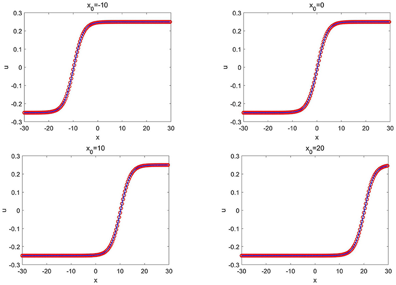
Figure 10. Ito's fifth order mKdV equation of Example 3.7: the CANN solution (red circles) and the exact solution (solid blue lines) at T = 1.0 with different x0 where κ = 0.25 is fixed.
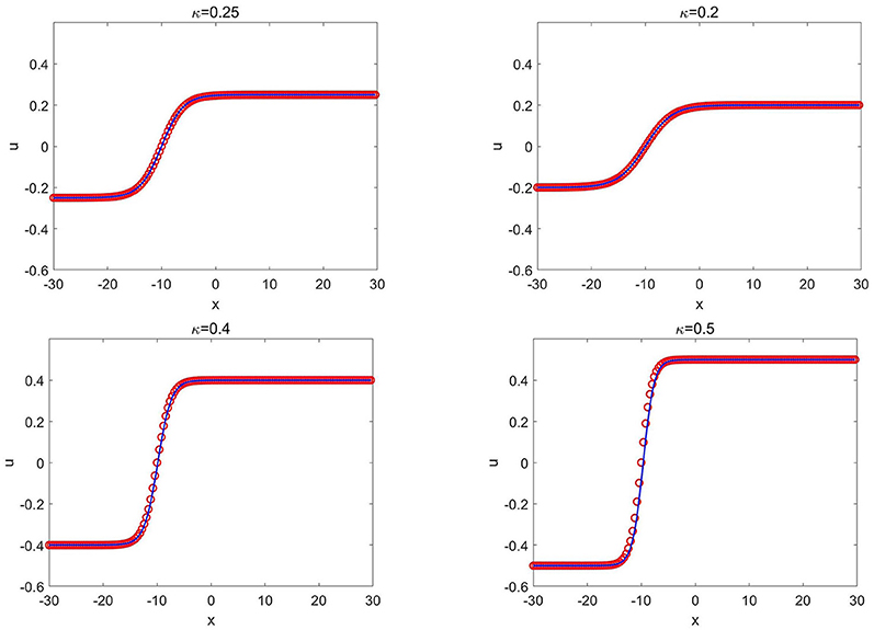
Figure 11. Ito's fifth order mKdV equation of Example 3.7: the CANN solution (red circles) and the exact solution (solid blue lines) at T = 1.0 with different κ where x0 = −10 is fixed.
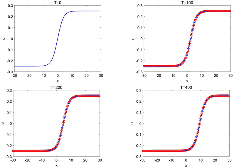
Figure 12. Ito's fifth order mKdV equation of Example 3.7: the CANN solution (red circles) and the exact solution (solid blue lines) at different time T with κ = 0.25 and x0 = 0.
Example 3.8. In this example, we consider the generalized fifth order KdV equation [52]
with δ = 0.16. The computational domain is taken as −10 ≤ x ≤ 20 and periodic boundary conditions are applied. This is a fifth order equation involving nonlinear first order, third order, and fifth order terms. We consider the following group of compacton solutions
where with the wave center x0 and the wave speed/amplitude λ being arbitrary constants.
The spatial mesh size Δx = 0.0125 and the time step size are taken to set up the CANN method. The network input vector
is chosen. The structure of the network consists of three hidden layers with 40 neurons in the first, 20 neurons in the second and 10 neurons in the third layers. The training data set is generated from the solution (3.23) with λ = 0.1 and x0 = −5. The total number of epoch iterations is set as K = 2 × 10⁵.
After well-trained, the network solver is applied to solve a group of compacton solutions (3.23) with different values of λ and x0. Figure 13 shows the CANN simulations with different values of λ while x0 = −5 is fixed. Figure 14 shows the CANN simulations with different values of x0 while λ = 0.1 is fixed. The CANN method can be generalized and accurately approximate the solutions (3.23) over the range 0.05 ≤ λ ≤ 0.2 and −5 ≤ x0 ≤ 15. We also test this example for long time simulation (up to T = 150) for the solution (3.23) with λ = 0.1 and x0 = 0 and plot the solutions at T = 0, 50, 100, and 150 in Figure 15. The CANN method can approximate the single compacton propagation well after long time simulation.
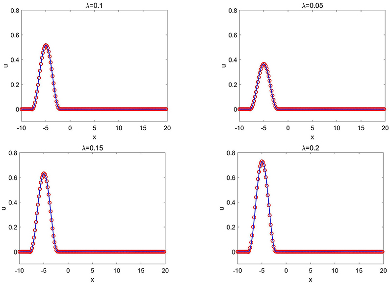
Figure 13. Generalized fifth order KdV equation of Example 3.8: the CANN solution (red circles) and the exact solution (solid blue lines) at T = 0.5 with different values of λ where x0 = −5 is fixed.
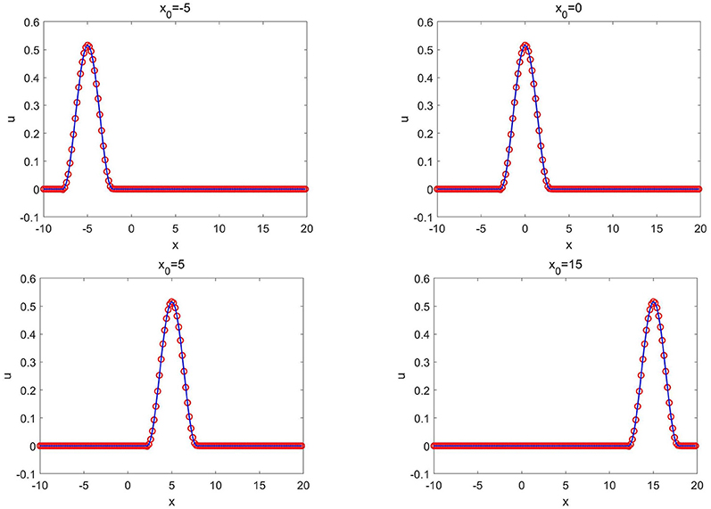
Figure 14. Generalized fifth order KdV equation of Example 3.8: the CANN solution (red circles) and the exact solution (solid blue lines) at T = 0.5 with different values of x0 where λ = 0.1 is fixed.
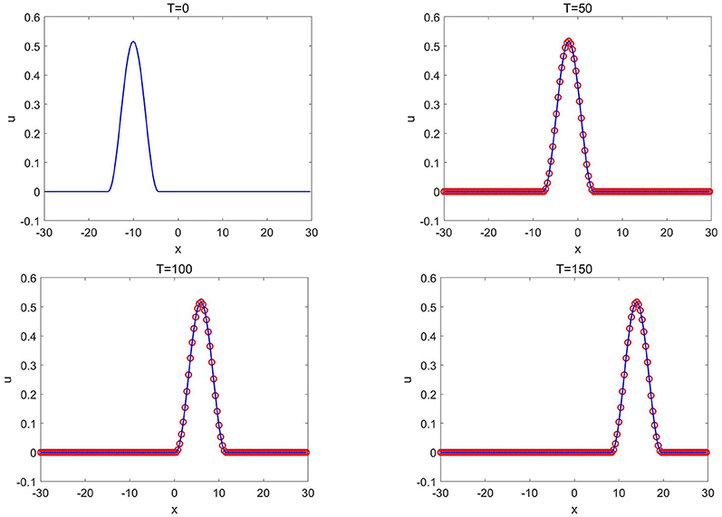
Figure 15. Generalized fifth order KdV equation of Example 3.8: the CANN solution (red circles) and the exact solution (solid blue lines) at different time T with x0 = 0 and λ = 0.1.
4. Conclusions
In this paper, we investigate the CANN method for solving four classes of KdV type equations involving third order or fifth order derivatives. This method is based on the integral formulation of the equation as the finite volume method and apply a feedforward network to learn the cell average between two consecutive time steps. The training data set is generated by one generic initial value of the given PDE, i.e., one single solution trajectory, and the training process uses multiple time levels (five time steps) of cell averages to maintain the stability and control the accumulation errors in time. Once well trained, the CANN solver can be applied to solve a group of initial values problems with insignificant generalization error. Numerical tests for four classes of the KdV equations are carried out to verify that the CANN method can be generalized to a group of PDEs with different wave amplitudes, different wave centers, or even different wave speed. Although this paper restricts on uniform mesh, it is worth mentioning that the proposed CANN method is a finite volume type neural network method which inherits the advantage and flexibility on geometry and thus can also work well on non-uniform regular mesh in space. Investigation on nonuniform temporal sizes and applications for more complicated nonlinear PDEs will be conducted in the future work.
Data availability statement
The original contributions presented in the study are included in the article/supplementary material, further inquiries can be directed to the corresponding author.
Author contributions
YC, JY, and XZ contributed to conception and design of the study. YC performed all the numerical simulations and wrote the first draft of the manuscript. JY and XZ revised critically for important content. All authors contributed to manuscript revision, read, and approved the submitted version.
Funding
Research work of JY was partially supported by the NSF grant DMS-1620335 and Simons Foundation grant 637716. Research work of XZ was partially supported by the NSFC Grant 11871428.
Conflict of interest
The authors declare that the research was conducted in the absence of any commercial or financial relationships that could be construed as a potential conflict of interest.
Publisher's note
All claims expressed in this article are solely those of the authors and do not necessarily represent those of their affiliated organizations, or those of the publisher, the editors and the reviewers. Any product that may be evaluated in this article, or claim that may be made by its manufacturer, is not guaranteed or endorsed by the publisher.
References
1. Qiu C, Yan J. Cell-average based neural network method for hyperbolic and parabolic partial differential equations. arXiv:210700813. (2021).
2. Korteweg DJ, de Vries G. On the change of form of long waves advancing in a rectangular canal, and on a new type of long stationary waves. Philos Mag Ser 5. (1895) 39:422–43. doi: 10.1080/14786449508620739
3. Su CH, Gardner CS. Korteweg-de Vries equation and generalizations. III. Derivation of the Korteweg-de Vries equation and Burgers equation. J Math Phys. (1969) 10:536–9. doi: 10.1063/1.1664873
4. Ito M. An extension of nonlinear evolution equations of the KdV (mKdV) type to higher orders. J Phys Soc Jpn. (1980) 49:771–8. doi: 10.1143/JPSJ.49.771
5. Yamamoto Y, Iti Takizawa E. On a solution on non-linear time-evolution equation of fifth order. J Phys Soc Jpn. (1981) 50:1421–2. doi: 10.1143/JPSJ.50.1421
6. Canosa J, Gazdag J. The Korteweg-de Vries-Burgers equation. J Comput Phys. (1977) 23:393–403. doi: 10.1016/0021-9991(77)90070-5
7. Bona JL, Dougalis VA, Karakashian OA, McKinney WR. Computations of blow-up and decay for periodic solutions of the generalized Korteweg-de Vries-Burgers equation. Appl Numer Math. (1992) 10:335–55. doi: 10.1016/0168-9274(92)90049-J
8. Yan J, Shu CW. A local discontinuous Galerkin method for KdV type equations. SIAM J Numer Anal. (2002) 40:769–91. doi: 10.1137/S0036142901390378
9. Xu Y, Shu CW. Local discontinuous Galerkin methods for three classes of nonlinear wave equations. J Comput Math. (2004) 22:250–74.
10. Ahmat M, Qiu J. Compact ETDRK scheme for nonlinear dispersive wave equations. Comput Appl Math. (2021) 40:286. doi: 10.1007/s40314-021-01687-0
11. E W. A proposal on machine learning via dynamical systems. Commun Math Stat. (2017) 5:1–11. doi: 10.1007/s40304-017-0103-z
12. Ruthotto L, Haber E. Deep neural networks motivated by partial differential equations. J Math Imaging Vis. (2020) 62:352–64. doi: 10.1007/s10851-019-00903-1
13. Rudy SH, Brunton SL, Proctor JL, Kutz JN. Data-driven discovery of partial differential equations. Sci Adv. (2017) 3:e1602614. doi: 10.1126/sciadv.1602614
14. Long Z, Lu Y, Dong B. PDE-Net 2.0: learning PDEs from data with a numeric-symbolic hybrid deep network. J Comput Phys. (2019) 399:108925. doi: 10.1016/j.jcp.2019.108925
15. Beck C, E W, Jentzen A. Machine learning approximation algorithms for high-dimensional fully nonlinear partial differential equations and second-order backward stochastic differential equations. J Nonlin Sci. (2019) 29:1563–619. doi: 10.1007/s00332-018-9525-3
16. Lye KO, Mishra S, Ray D. Deep learning observables in computational fluid dynamics. J Comput Phys. (2020) 410:109339. doi: 10.1016/j.jcp.2020.109339
17. Khoo Y, Lu J, Ying L. Solving parametric PDE problems with artificial neural networks. Eur J Appl Math. (2021) 32:421–35. doi: 10.1017/S0956792520000182
18. Chan S, Elsheikh AH. A machine learning approach for efficient uncertainty quantification using multiscale methods. J Comput Phys. (2018) 354:493–511. doi: 10.1016/j.jcp.2017.10.034
19. Zhu Y, Zabaras N. Bayesian deep convolutional encoder–decoder networks for surrogate modeling and uncertainty quantification. J Comput Phys. (2018) 366:415–47. doi: 10.1016/j.jcp.2018.04.018
20. Tripathy RK, Bilionis I. Deep UQ: learning deep neural network surrogate models for high dimensional uncertainty quantification. J Comput Phys. (2018) 375:565–88. doi: 10.1016/j.jcp.2018.08.036
21. Zhang D, Lu L, Guo L, Karniadakis GE. Quantifying total uncertainty in physics-informed neural networks for solving forward and inverse stochastic problems. J Comput Phys. (2019) 397:108850. doi: 10.1016/j.jcp.2019.07.048
22. Winovich N, Ramani K, Lin G. ConvPDE-UQ: convolutional neural networks with quantified uncertainty for heterogeneous elliptic partial differential equations on varied domains. J Comput Phys. (2019) 394:263–79. doi: 10.1016/j.jcp.2019.05.026
23. Zhao Y, Mao Z, Guo L, Tang Y, Karniadakis GE. A spectral method for stochastic fractional PDEs using dynamically-orthogonal/bi-orthogonal decomposition. J Comput Phys. (2022) 461:111213. doi: 10.1016/j.jcp.2022.111213
24. Guo L, Wu H, Zhou T. Normalizing field flows: solving forward and inverse stochastic differential equations using physics-informed flow models. J Comput Phys. (2022) 461:111202. doi: 10.1016/j.jcp.2022.111202
25. Ray D, Hesthaven JS. An artificial neural network as a troubled-cell indicator. J Comput Phys. (2018) 367:166-191. doi: 10.1016/j.jcp.2018.04.029
26. Wang Y, Shen Z, Long Z, Dong B. Learning to discretize: solving 1D scalar conservation laws via deep reinforcement learning. Commun Comput Phys. (2020) 28:2158–79. doi: 10.4208/cicp.OA-2020-0194
27. Sun Z, Wang S, Chang LB, Xing Y, Xiu D. Convolution neural network shock detector for numerical solution of conservation laws. Commun Comput Phys. (2020) 28:2075–108. doi: 10.4208/cicp.OA-2020-0199
28. Yu X, Shu CW. Multi-layer perceptron estimator for the total variation bounded constant in limiters for discontinuous Galerkin methods. La Matemat. (2022) 1:53–84. doi: 10.1007/s44007-021-00004-9
29. Cybenko G. Approximation by superpositions of a sigmoidal function. Math Control Signals Syst. (1989) 2:303–14. doi: 10.1007/BF02551274
30. Barron AR. Universal approximation bounds for superpositions of a sigmoidal function. IEEE Trans Inform Theory. (1993) 39:930–45. doi: 10.1109/18.256500
31. Leshno M, Lin VY, Pinkus A, Schocken S. Multilayer feedforward networks with a nonpolynomial activation function can approximate any function. Neural Netw. (1993) 6:861–7. doi: 10.1016/S0893-6080(05)80131-5
32. Lagaris I, Likas A, Fotiadis D. Artificial neural networks for solving ordinary and partial differential equations. IEEE Trans Neural Netw. (1998) 95:987–1000. doi: 10.1109/72.712178
33. Rudd K, Ferrari S. A constrained integration (CINT) approach to solving partial differential equations using artificial neural networks. Neurocomputing. (2015) 155:277–85. doi: 10.1016/j.neucom.2014.11.058
34. Berg J, Nyström K. A unified deep artificial neural network approach to partial differential equations in complex geometries. Neurocomputing. (2018) 317:28–41. doi: 10.1016/j.neucom.2018.06.056
35. Sirignano J, Spiliopoulos K. DGM: a deep learning algorithm for solving partial differential equations. J Comput Phys. (2018) 375:1339–64. doi: 10.1016/j.jcp.2018.08.029
36. Zang Y, Bao G, Ye X, Zhou H. Weak adversarial networks for high-dimensional partial differential equations. J Comput Phys. (2020) 411:109409. doi: 10.1016/j.jcp.2020.109409
37. Cai Z, Chen J, Liu M. Least-squares ReLU neural network (LSNN) method for linear advection-reaction equation. J Comput Phys. (2021) 2021:110514. doi: 10.1016/j.jcp.2021.110514
38. Raissi M, Perdikaris P, Karniadakis GE. Physics-informed neural networks: a deep learning framework for solving forward and inverse problems involving nonlinear partial differential equations. J Comput Phys. (2019) 378:686–707. doi: 10.1016/j.jcp.2018.10.045
39. Raissi M. Deep hidden physics models: Deep learning of nonlinear partial differential equations. J Mach Learn Res. (2018) 19:932–55.
40. Raissi M, Yazdani A, Karniadakis GE. Hidden fluid mechanics: learning velocity and pressure fields from flow visualizations. Science. (2020) 367:1026–30. doi: 10.1126/science.aaw4741
41. Sun Y, Zhang L, Schaeffer H. NeuPDE: Neural network based ordinary and partial differential equations for modeling time-dependent data. In: Proceedings of The First Mathematical and Scientific Machine Learning Conference. (2020). p. 352–72.
42. Li Y, Lu J, Mao A. Variational training of neural network approximations of solution maps for physical models. J Comput Phys. (2020) 409:109338. doi: 10.1016/j.jcp.2020.109338
43. Lu Y, Wang L, Xu W. Solving multiscale steady radiative transfer equation using neural networks with uniform stability. Res Math Sci. (2022) 45:9. doi: 10.1007/s40687-022-00345-z
44. Li Z, Kovachki NB, Azizzadenesheli K, Liu B, Bhattacharya K, Stuart AM, et al. Neural operator: graph Kernel network for partial differential equations. In: ICLR 2020 Workshop on Integration of Deep Neural Models and Differential Equations. (2020).
45. Li Z, Kovachki NB, Azizzadenesheli K, Liu B, Bhattacharya K, Stuart AM, et al. Fourier neural operator for parametric partial differential equations. In: International Conference on Learning Representations. (2020).
46. Wu K, Xiu D. Data-driven deep learning of partial differential equations in modal space. J Comput Phys. (2020) 408:109307. doi: 10.1016/j.jcp.2020.109307
47. Bilotta E, Pantano P. Cellular nonlinear networks meet KdV equation: a new paradigm. Int J Bifurc Chaos. (2013) 23:1330003–8125. doi: 10.1142/S0218127413300036
48. Shen Z, Yang H, Zhang S. Neural network approximation: three hidden layers are enough. Neural Netw. (2021) 141:160–73. doi: 10.1016/j.neunet.2021.04.011
49. Loshchilov I, Hutter F. Decoupled weight decay regularization. In: International Conference on Learning Representations. (2018).
50. Debussche A, Printems J. Numerical simulation of the stochastic Korteweg-de Vries equation. Phys D. (1999) 134:200–26. doi: 10.1016/S0167-2789(99)00072-X
51. Rosenau P, Hyman JM. Compactons: solitons with finite wavelength. Phys Rev Lett. (1993) 70:564-567. doi: 10.1103/PhysRevLett.70.564
52. Rosenau P, Levy D. Compactons in a class of nonlinearly quintic equations. Phys Lett A. (1999) 252:297–306. doi: 10.1016/S0375-9601(99)00012-2
Keywords: neural network, finite volume method, KdV equations, nonlinear dispersive equations, CANN method
Citation: Chen Y, Yan J and Zhong X (2022) Cell-average based neural network method for third order and fifth order KdV type equations. Front. Appl. Math. Stat. 8:1021069. doi: 10.3389/fams.2022.1021069
Received: 17 August 2022; Accepted: 17 October 2022;
Published: 07 November 2022.
Edited by:
Li Wang, University of Minnesota Twin Cities, United StatesReviewed by:
Juntao Huang, Michigan State University, United StatesOmar Abu Arqub, Al-Balqa Applied University, Jordan
Copyright © 2022 Chen, Yan and Zhong. This is an open-access article distributed under the terms of the Creative Commons Attribution License (CC BY). The use, distribution or reproduction in other forums is permitted, provided the original author(s) and the copyright owner(s) are credited and that the original publication in this journal is cited, in accordance with accepted academic practice. No use, distribution or reproduction is permitted which does not comply with these terms.
*Correspondence: Xinghui Zhong, emhvbmd4aEB6anUuZWR1LmNu