 Getu Mekonnen Wondimu
 Mesfin Mekuria Woldaregay
 Tekle Gemechu Dinka
 Gemechis File Duressa2
94% of researchers rate our articles as excellent or good
Learn more about the work of our research integrity team to safeguard the quality of each article we publish.
Find out more
ORIGINAL RESEARCH article
Front. Appl. Math. Stat., 25 October 2022
Sec. Numerical Analysis and Scientific Computation
Volume 8 - 2022 | https://doi.org/10.3389/fams.2022.1005330
This article is part of the Research Topic2022 Applied Mathematics and Statistics – Editor’s PickView all 15 articles
This paper presents numerical treatments for a class of singularly perturbed parabolic partial differential equations with nonlocal boundary conditions. The problem has strong boundary layers at x = 0 and x = 1. The nonstandard finite difference method was developed to solve the considered problem in the spatial direction, and the implicit Euler method was proposed to solve the resulting system of IVPs in the temporal direction. The nonlocal boundary condition is approximated by Simpsons rule. The stability and uniform convergence analysis of the scheme are studied. The developed scheme is second-order uniformly convergent in the spatial direction and first-order in the temporal direction. Two test examples are carried out to validate the applicability of the developed numerical scheme. The obtained numerical results reflect the theoretical estimate.
Differential equations that involve a small parameter in their higher order derivative term are said to be singularly perturbed problems (SPPs) or singularly perturbed differential equations (SPDEs). Many mathematical models, starting from fluid dynamics to mathematical biology, are modeled using (SPPs). For example, high Reynold's number flow in fluid dynamics, heat transport problems with large Péclet numbers, elastic vibration, etc. [1] and the references therein. Such mathematical problems are extremely difficult to solve exactly. Thus, for treating such problems numerical methods are preferable. Various scientific and engineering processes can be modeled as integral terms over the spatial domain that appear inside or outside of the boundary conditions [2, 3]. Such problems are said to be nonlocal problems. Many physical phenomena are formulated as nonlocal mathematical models. For instance, problems in thermodynamics [4], plasma physics [5], heat conduction [6], underground water flow, and populace dynamics [7] can be reduced to nonlocal problems with integral conditions. SPPs having nonlocal boundary conditions in which the highest order derivative term is multiplied by way of a small parameter are referred to as SPPs with integral boundary conditions. Such problems exhibit boundary layer phenomena wherein the solution changes. However, the numerical treatments of SPPs attract the attention of researchers due to the boundary layer behavior of the solution. Since the small parameter multiplies the highest derivative, the small regions adjoin the domain of interest's boundaries or any interior stage at which the variable quantity undergoes a very unexpected change. As a result, these problems have strong boundary layers, which ensures that there are small areas where the solution rapidly changes within very small layers near the boundary or within the problem domain [8]. Numerically treating such SPPs with nonlocal boundary conditions is a challenging task due to a very small perturbation parameter (ε).
In recent times, a class of SPPs involving nonlocal boundary conditions have been obtained great attention from scholars. To mention few of them, the authors in Bahuguna and Dabas [9], Feng et al. [10], and Li and Sun [11] studied the existence and uniqueness of a class of SPPs with nonlocal boundary conditions. The authors in Raja and Tamilselvan [12] developed a finite difference scheme for solving a class of a system of singularly perturbed reaction diffusion equations with integral boundary conditions. Debala and Duressa [13] built a uniformly convergent numerical scheme for solving SPPs with nonlocal boundary conditions. Numerical methods for solving singularly perturbed delay differential equations (SPDDEs) are considered in Sekar and Tamilselvan [14–17]. The authors developed finite difference schemes with suitable piecewise uniform Shiskin meshes. The authors in Debela and Duressa [18] used an exponentially fitted numerical scheme to solve SPDDEs of the convection-diffusion kind with nonlocal boundary conditions. Debela and Duressa [19] improved the order of accuracy for the method proposed in Debela and Duressa [18]. Kumar and Kumari [20] developed the method based on the idea of B-spline functions and an efficient numerical method on a piecewise-uniform mesh was recommended to approximate the solutions of SPPs having a delay of unit magnitude with an integral boundary condition. In the literature, only few authors considered a class of singularly perturbed parabolic partial differential equations (SPPPDEs) with integral boundary conditions. Sekar and Tamislevan [21] investigate a numerical solution for singularly perturbed delay partial differential equations (SPDPDEs) of the reaction-diffusion type with integral boundary conditions. They developed the standard finite difference on a rectangular piecewise uniform mesh for spatial discretization and a backward difference scheme in time derivative. Gobena and Duressa [22] constructed and analyzed an accurate numerical method for solving SPDPDEs with integral boundary conditions.
In general, the classical numerical methods used for solving SPDEs are not well-posed and fail to provide an exact solution when a perturbation parameter (ε) goes to zero. Therefore, it is essential to develop a numerical method that offers suitable results for small values of the perturbation parameter. As far as the researchers' knowledge, singularly perturbed parabolic partial differential equations with nonlocal boundary conditions are first being considered and have not yet been treated numerically. In this study, we investigate a uniformly convergent numerical method for solving the problem under consideration. We used the nonstandard finite difference method for space direction and the implicit Euler method for time direction.
The contents of the paper are arranged in the following manner: A brief introduction of the given problem is discussed in Section 1. In Section 2, the properties of continuous solutions are given. In Section 3, a numerical method is formulated by using the method of lines for the given problem. Stability and convergence analysis for developed numerical methods are also studied. Numerical results and discussions are given in Section 4. In Section 5, the conclusion of the paper is given.
Notation: In this paper, N and M denote the number of mesh intervals in spatial and temporal discretization, respectively. C is a generic positive constant independent of ε, N, and M. The norm used for studying the convergence of numerical solutions is the maximum norm defined as ||z(s, t)||: = sup|z(s, t)|, (s, t) ∈ D.
In this paper, we consider a class of singularly perturbed 1D parabolic partial differential equations of the reaction-diffusion type with non-local boundary conditions,
where and ε is a small parameter (0 < ε ≪ 1). Suppose that a(s, t) ≥ α > 0, f(s, t), ϕl, ϕr, ϕb are sufficiently smooth functions and g(s) is nonnegative monotone function and satisfies . The existence and uniqueness of the problem (1) can be established under the assumption that the data are Hölder continuous and imposing proper compatibility conditions at the corners [23]. Note that ϕl and ϕr are only functions of t, while ϕb is a function of x only. The problems necessarily satisfies the following sufficient compatibility conditions ϕb(0, 0) = ϕl(0, 0), ϕb(1, 0) = ϕr(1, 0), and
Note that ϕl, ϕr, and ϕb are assumed to be sufficiently smooth for Equation (1) to make sense, namely , and .
Next, we analyze some properties of the continuous solution (Equation 1) which guarantee the existence and uniqueness of the analytical solution. A replication of this belonging in semi-discrete form can be used to present the approximate solution, which we provide in the following section.
Lemma 1. (Continuous Maximum Principle) Let be a sufficiently smooth function such that . Then Ψ(s, t) ≥ 0, , where .
Proof. Assume (s*, t*) be defined as and suppose that Ψ(s*, t*) ≤ 0. It is known that (s*, t*) ∉ ∂D. Thus, . Since , which indicates that Ψ(s*, t*) = 0, , and implies that , which is contradicts with the above assumption. . So that, Ψ(s, t) ≥ 0, ∀(s, t) ∈ D. □
Lemma 2. (Stability Result) Assume z(s, t) is the solution to the continuous problem in Equation (1). Then we have the bound
where ||f|| = max{f(s, t)}.
Proof. We prove this by using the maximum principle Lemma (1) and by constructing the barrier functions , where . At initial, we have
For x = 0, we have
For x = 1, we have
For 0 < s < 1, we have
where ε > 0, a(s, t) ≥ α > 0. This implies that . Hence, by Lemma 1, we have, , which indicates
□
The sufficient conditions for the existence of a unique solution is given in Lemma 3 and Theorem 1.
Lemma 3. If the coefficient satisfies and boundary conditions satisfies and suppose that the compatibility conditions are satisfied. Then, the problem (Equation 1) has a unique solution z(s, t) which is satisfy .
Proof. Refer to Ladyženskaja et al. [23] □
To estimate the error for the fitted numerical technique below, the idea that the solution of Equation (1) is more regular than the one guaranteed by using the result in Theorem 1. To attain this greater regularity, stronger compatibility conditions are imposed at the corners.
Theorem 1. If the coefficient satisfies and boundary conditions satisfies , Then the problem (Equation 1) having a unique solution z which satisfies . And also the derivatives of solution z are bounded, ∀i, j ∈ Z ≥ 0 such that 0 ≤ i + 2j ≤ 4,
Proof. The boundedness of the solutions and its derivative is given as follows. Under the stretched transformation problem (Equation 1) can be rewritten as
where , and the boundary condition to Γ, where Equation (2) is independent of ε. Then, by taking the idea of estimation (10.6) of Ladyženskaja et al. [23] (p. 352), we will obtain
∀ Ñδ in . Here, Ñδ, δ > 0 is a neighborhood with diameter δ in . Returning to the original variable
Hence, the proof is complete by using the bound on z of Lemma 2. □
The bounds of the derivatives of the solution given in Theorem 1 were derived from classical results. They are not adequate for the proof of the ε -uniform error estimate. Stronger bounds on these derivatives are now obtained by a method originally devised in Shishkin [24]. The main idea is to decompose the solution z into smooth and singular components.
Lemma 4. If the coefficient satisfies , and the boundary conditions satisfies . Then we have
where C is a constant independent of parameter ε,
Proof. For proof, the interested reader can refer to Elango et al. [21]. □
The fundamental idea of non-standard discrete modeling techniques is the development of the exact finite difference technique. Micken presented methods and rules for developing nonstandard FDMs for various types of problems [25]. To develop a discrete scheme in keeping with Mickens' guidelines, the denominator characteristic for the discrete derivatives should be described in terms of more complicated functions with larger step sizes than those used in classical methods. These complicated functions are a general property of the method that may be useful when constructing dependable methods for such problems.
To construct a genuine finite difference scheme for the problem of the form in Equation (1), we use the methods described in Woldaregay and Duressa [26]. The constant coefficient given in Equation (3) without the time variable is considered as follows.
By solving Equation (3), we obtain two independent solutions and , where
The spatial domain [0, 1] is discretized on uniform mesh length Δs = h as follows. , N is taken as number of mesh points in the spatial discretization. The approximate solution of z(si) will be denoted by Zi. Here, the main aim is to compute difference equations that have similar results with the problem (Equation 1) at the mesh point si which is given by . Applying the procedures given in Mickens [25], we get
After simplification, Equation (4) becomes
which is an exact difference scheme for Equation (3). By performing some arithmetic manipulation and making rearrangement on Equation (5) for the variable coefficient problem, we obtain
The denominator function becomes
where λ2 is a function of ε, βi, h, and .
For more information about nonstandard finite difference methods for reaction diffusion problems, an interested reader can refer to the study of Munyakazi and Patidar [27].
By using Equation (7), and applying the nonstandard finite difference method to a semi-discrete problem, we have
with boundary conditions
Here, for i = N, the integral boundary condition approximated by composite Simpson's integration rule.
Substituting Equation (10) in to Equation (9), we obtain
Equation (11) can be rewritten as
Assume that the approximation of z(si, t) is denoted as Zi(t), by using the non-standard finite difference approximation. At this level, Equation (1) is reduced in the form of semi-discrete as follows.
Equation (12) is the system of IVPs and its compact form is written as
where B is (N − 1) × (N − 1) tridiagonal matrix, Zi(t) and Fi(t) are (N − 1) entries of the column vector. The entries of B and F respectively given as
and
Here, we present the maximum principle and uniform stability estimate of the semi-discrete operator and its convergence analysis.
Lemma 5. (Semi-discrete Maximum Principle): Assume that Z0(t) ≥ 0, . Then ∀ i = 1(1)N − 1, implies that Zi(t) ≥ 0 ∀ i = 0(1)N.
Proof. Assume there exists q ∈ {0, ⋯ , N} such that . Suppose Zq(t) ≤ 0, which implies q ≠ 0, N. Also, we have Zq+1 − Zq > 0 and Zq − Zq−1 < 0. Here, we have
By using the above assumption, we get that , for i = 1(1)N − 1. Thus, the assumption Zi(t) < 0, i = 0(1)N is not correct. Hence, Zi(t) ≥ 0 ∀ i = 0(1)N. □
This Lemma 5 is used to obtain the bounds of the discrete solution given in Lemma 6. In general, the discrete maximum principle is widely used to show the boundedness and positivity of a discrete solution.
Lemma 6. The solution Zi(t) of the semidiscrete problem in Equations (12) or (13) satisfies the following bound.
Proof. Suppose and define a comparison function as
For the points on the boundary, we have
For 1 ≤ i ≤ N − 1, we have
From Lemma 5, we get, , ∀ . □
Next, we present the convergence analysis of spatial discretization. We denoted Zi(t) as approximate solution for the spatial semidiscretization to the exact solution z(s, t) at s = si, i = 0(1)N. Let us define the backward and forward finite differences in space as:
respectively, and the second order central finite difference operator as
Lemma 7. Let N be a fixed mesh. Then, for ε → 0, we have
where m = 1, 2, 3, ⋯ .
Proof. Refer to Munyakazi and Patidar [27] □
Theorem 2. Let the coefficient function a(s) and the function f(s, t) in Equation (12) be sufficiently smooth and . Then the semidiscrete solution Zi(t) of Equation (12) satisfies
Proof. The truncation error in spatial direction is considered as
Note that we have used Taylor expansions of zi−1(t) and zi+1(t). A truncated Taylor expansion of of order five becomes
Using Equation (15) in Equation (14), we obtain
We use Lemma (7), to obtain the boundedness of Equation (16). Using Lemma (7) and Theorem (1), we obtain
The truncation error at s = sN, become
Theorem 3. The semidiscrete solutions satisfy the uniform error bound
Proof. The proof follows from Theorem (1) and Lemma (7) under the properties of boundedness of a semi-discrete solution and the required bound is satisfied.
A mesh with length Δt = tj+1 − tj,j = 0(1)M − 1 is constructed on the time domain Dt = [0, T], where M is a positive integer. The IVPs Equation (13) are discretized using the implicit Euler method on a uniform mesh. By denoting the approximation of zi(tj) as , we construct the time discretization as follows.
with the initial condition Z0(t) = ϕl(tj), and by rearranging Equation (19), we obtain
Lemma 8. Suppose Then the local truncation error associated with the time direction satisfies
Proof. The local truncation error is defined as
Using Taylor expansion, we obtain z(tj−1) as
However, zt(tj) = F(tj) − B(tj)z(tj). Thus,
Now, the local truncation error ej becomes
Since the matrix B is invertible, using the relation (Δt)2 > (Δt)3 for small Δt and z(tj) ≤ C, we obtain
□
Lemma 9. The global error estimate in the time direction is given by ||Ej+1|| ≤ CΔt, ∀j ≤ T/Δt, where .
Proof. The global error estimate at (j+1)th time step is obtained by using the local error estimate up to jth time step as follows.
Hence,
where C is a positive constant independent of ε and Δt. By taking the supremum ∀ ε ∈ (0, 1], we obtained
□
We summarizes the results of this work by considering the error estimate obtained in Equations (18) and (22) and we conclude by the following theorem.
Theorem 4. The error estimate for the solution of the continuous and fully discrete problems is given by
where z(s, t) and are the solutions to problems Equations (1) and (12), respectively.
Proof. The error estimation of the fully discrete scheme is given as follows.
Then, by combining the bound given in Theorem 3 and Lemma 9, the theorem gets proved.
Here, we developed an algorithm for the proposed method for the problem and perform experiments to validate the theoretical justifications and results. Since the exact solutions of the given examples are not known, we use double mesh techniques to obtain the maximum pointwise error of the developed scheme. Now, let UN,Δt be a conducted solution of a problem using mesh points N and time step size Δt. Again, be a conducted solution on double mesh points of 2N and half of time step size Δt/2.
We calculate the maximum absolute error as and the parameter uniform error estimate by using We calculate the rate of convergence of the developed scheme by using The parameter rate of convergence is calculated as
Example 1.
Example 2.
The solutions of the above two examples exhibit strong boundary layers near x = 0 and x = 1. We presented the surface plots for numerical solutions of Examples 1 and 2 in Figures 1, 2 respectively, which display the presence of boundary layers formation on the left and right side of the spatial domain for different values of ε. The maximum pointwise error and rate of convergence of the proposed schemes of Examples 1 and 2 are given in Tables 1, 2 respectively for various values of the perturbation parameter ε, mesh number N and time step size Δt. From these tables, one can observe that the developed scheme is parameter uniform convergent, which supports the theoretical results. Figure 3 indicates the Log-Log plots for the maximum absolute error vs. mesh number N for the singular perturbation parameter ε. One can observe that as ε goes very small, the developed method converges uniformly independent of the perturbation parameter ε.
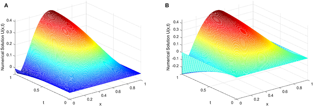
Figure 1. 3-D graph of numerical solution for Example (1) which displays the existing layer. (A) ε = 10−2. (B) ε = 10−12.
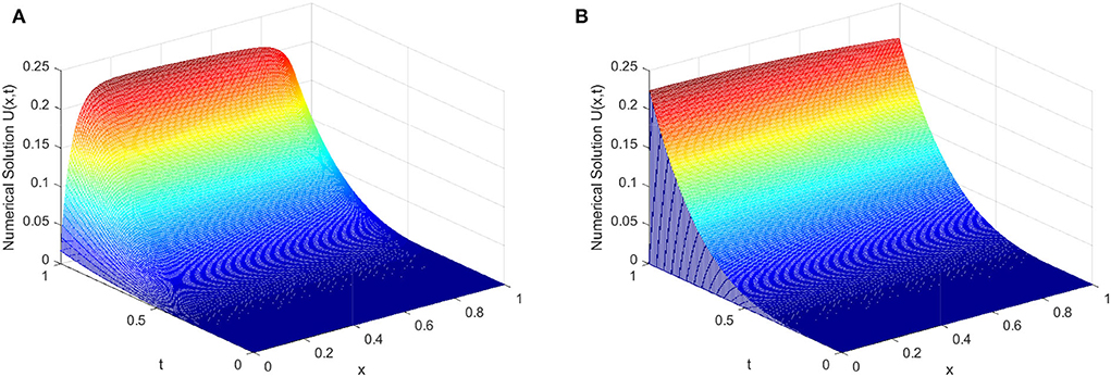
Figure 2. 3-D graph of numerical solution for Example (2) that displays the existing layer. (A) ε = 10−2. (B) ε = 10−12.
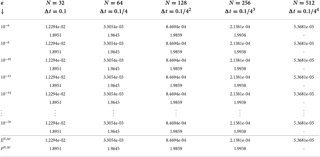
Table 1. Maximum absolute error and rate of convergence of the scheme for Example (1).
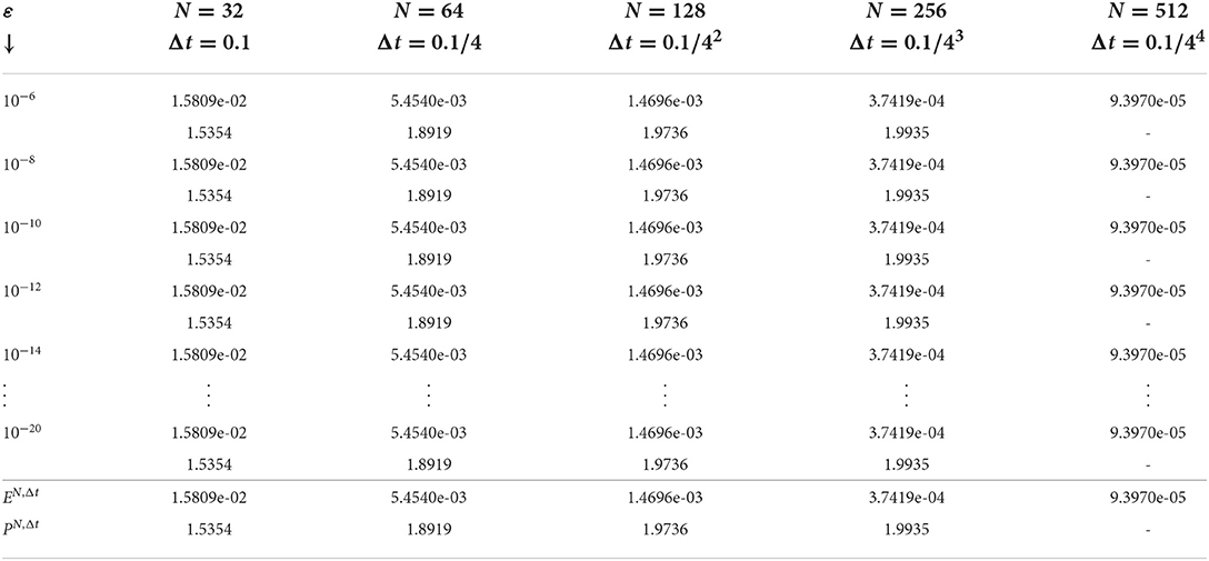
Table 2. Maximum absolute error and rate of convergence of the scheme for Example (2).
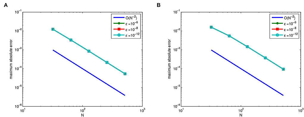
Figure 3. The Log-Log plot of the maximum absolute error for different values of ε for Examples 1 and 2, respectively. (A) Log-Log plot for Example (1). (B) Log-Log plot for Example (2).
This paper investigates a numerical treatment for a class of singularly perturbed parabolic partial differential equations of the reaction-diffusion type with nonlocal boundary conditions. To solve the problem at hand, we employed the method of lines. A nonstandard finite difference scheme is used to semi-discretize the spatial direction, and the implicit Euler method is used to discretize the results of initial value problems. To deal with the integral boundary condition, we used a composite Simpson's rule. The stability of the evolved numerical scheme is established, and the scheme's uniform convergence is demonstrated. To validate the problem's applicability, two test examples are carried out for numerical computation for different values of the perturbation parameter ε and mesh points. The entire procedure has been demonstrated to be second-order uniformly convergent in the spatial direction and first-order in the temporal direction. The theoretical estimation is reflected in our numerical results.
The original contributions presented in the study are included in the article/supplementary material, further inquiries can be directed to the corresponding author.
All authors listed have made a substantial, direct, and intellectual contribution to the work and approved it for publication.
Authors are grateful to their reviewers for their contributions.
The authors declare that the research was conducted in the absence of any commercial or financial relationships that could be construed as a potential conflict of interest.
All claims expressed in this article are solely those of the authors and do not necessarily represent those of their affiliated organizations, or those of the publisher, the editors and the reviewers. Any product that may be evaluated in this article, or claim that may be made by its manufacturer, is not guaranteed or endorsed by the publisher.
1. Kumar M, Paul. Methods for solving singular perturbation problems arising in science and engineering. Math Comput Model. (2011) 54:556–75. doi: 10.1016/j.mcm.2011.02.045
2. Dehghan M, Tatari M. Use of radial basis functions for solving the second-order parabolic equation with nonlocal boundary conditions. Math Comput Simulat. (2008) 24:924–38. doi: 10.1002/num.20297
3. Amiraliyev G, Amiraliyeva I, Kudu M. A numerical treatment for singularly perturbed differential equations with integral boundary condition. Appl Math Comput. (2007) 185:574–82. doi: 10.1016/j.amc.2006.07.060
4. Day W. Extensions of a property of the heat equation to linear thermoelasticity and other theories. Q Appl Math. (1982) 40:319–30. doi: 10.1090/qam/678203
5. Bouziani A. Mixed problem with boundary integral conditions for a certain parabolic equation. J Appl Math Stochastic Anal. (1996) 9:323–30. doi: 10.1155/S1048953396000305
6. Cannon J. The solution of the heat equation subject to the specification of energy. Q Appl Math. (1963) 21:155–60. doi: 10.1090/qam/160437
7. Kudu M, Amiraliyev GM. Finite difference method for a singularly perturbed differential equations with integral boundary condition. Int J Math Comput. (2015) 26:71–9.
8. OMalley RE. Ludwig prandtls boundary layer theory. In: Historical Developments in Singular Perturbations. Springer (2014). p. 1–26.
9. Bahuguna D, Dabas J. Existence and uniqueness of a solution to a semilinear partial delay differential equation with an integral condition. Nonlinear Dyn Syst Theory. (2008) 8:7–19.
10. Feng M, Ji D, Ge W. Positive solutions for a class of boundary-value problem with integral boundary conditions in Banach spaces. J Comput Appl Math. (2008) 222:351–63. doi: 10.1016/j.cam.2007.11.003
11. Li H, Sun F. Existence of solutions for integral boundary value problems of second-order ordinary differential equations. Boundary Value Problems. (2012) 2012:1–7. doi: 10.1186/1687-2770-2012-147
12. Raja V, Tamilselvan A. Fitted finite difference method for third order singularly perturbed convection diffusion equations with integral boundary condition. Arab J Math Sci. (2019) 25:231–42. doi: 10.1016/j.ajmsc.2018.10.002
13. Debela, Duressa GF. Uniformly convergent numerical method for singularly perturbed convection-diffusion type problems with nonlocal boundary condition. Int J Num Methods Fluids. (2020) 92:1914–26. doi: 10.1002/fld.4854
14. Sekar E, Tamilselvan A. Finite difference scheme for singularly perturbed system of delay differential equations with integral boundary conditions. J Korean Soc Ind Appl Math. (2018) 22:201–15. doi: 10.12941/jksiam.2018.22.201
15. Sekar E, Tamilselvan A. Finite difference scheme for third order singularly perturbed delay differential equation of convection diffusion type with integral boundary condition. J Appl Math Comput. (2019) 61:73–86. doi: 10.1007/s12190-019-01239-0
16. Sekar E, Tamilselvan A. Singularly perturbed delay differential equations of convection-diffusion type with integral boundary condition. J Appl Math Comput. (2019) 59:701–22. doi: 10.1007/s12190-018-1198-4
17. Sekar E, Tamilselvan A. Third order singularly perturbed delay differential equation of reaction diffusion type with integral boundary condition. J Appl Math Comput Mech. (2019) 18:99–110. doi: 10.17512/jamcm.2019.2.09
18. Debela, Duressa GF. Exponentially fitted finite difference method for singularly perturbed delay differential equations with integral boundary condition. Int J Eng Appl Sci. (2019) 11:476–93. doi: 10.24107/ijeas.647640
19. Debela, Duressa GF. Accelerated fitted operator finite difference method for singularly perturbed delay differential equations with non-local boundary condition. J Egypt Math Soc. (2020) 28:1–16. doi: 10.1186/s42787-020-00076-6
20. Kumar D, Kumari P. A parameter-uniform collocation scheme for singularly perturbed delay problems with integral boundary condition. J Appl Math Comput. (2020) 63:813–28. doi: 10.1007/s12190-020-01340-9
21. Elango S, Tamilselvan A, Vadivel R, Gunasekaran N, Zhu H, Cao J, et al. Finite difference scheme for singularly perturbed reaction diffusion problem of partial delay differential equation with nonlocal boundary condition. Adv Diff Equat. (2021) 2021:1–20. doi: 10.1186/s13662-021-03296-x
22. Gobena WT, Duressa GF. Parameter-uniform numerical scheme for singularly perturbed delay parabolic reaction diffusion equations with integral boundary condition. Int J Diff Equat. (2021) 2021:9993644. doi: 10.1155/2021/9993644
23. Ladyženskaja OA, Solonnikov VA, Ural'ceva NN. Linear and quasi-linear equations of parabolic type. In: American Mathematical Society, Vol. 23. Petersburg, VA (1988).
24. Shishkin GI. Approximation of the solutions of singularly perturbed boundary-value problems with a parabolic boundary layer. USSR Comput Math Math Phys. (1989) 29:1–10. doi: 10.1016/0041-5553(89)90109-2
25. Mickens RE. Advances in the applications of nonstandard finite difference schemes. In: World Scientific. (2005).
26. Woldaregay MM, Duressa GF. Uniformly convergent numerical method for singularly perturbed delay parabolic differential equations arising in computational neuroscience. Kragujevac J Math. (2022) 46:65–84. doi: 10.46793/KgJMat2201.065W
Keywords: singularly perturbed problems, partial differential equations, reaction-diffusion, method of lines, uniform convergence, nonlocal boundary condition
Citation: Wondimu GM, Woldaregay MM, Dinka TG and Duressa GF (2022) Numerical treatment of singularly perturbed parabolic partial differential equations with nonlocal boundary condition. Front. Appl. Math. Stat. 8:1005330. doi: 10.3389/fams.2022.1005330
Received: 28 July 2022; Accepted: 03 October 2022;
Published: 25 October 2022.
Edited by:
Lijian Jiang, Tongji University, ChinaReviewed by:
Majid Darehmiraki, Behbahan Khatam Alanbia University of Technology, IranCopyright © 2022 Wondimu, Woldaregay, Dinka and Duressa. This is an open-access article distributed under the terms of the Creative Commons Attribution License (CC BY). The use, distribution or reproduction in other forums is permitted, provided the original author(s) and the copyright owner(s) are credited and that the original publication in this journal is cited, in accordance with accepted academic practice. No use, distribution or reproduction is permitted which does not comply with these terms.
*Correspondence: Mesfin Mekuria Woldaregay, bXNmbm1rcjAyQGdtYWlsLmNvbQ==
Disclaimer: All claims expressed in this article are solely those of the authors and do not necessarily represent those of their affiliated organizations, or those of the publisher, the editors and the reviewers. Any product that may be evaluated in this article or claim that may be made by its manufacturer is not guaranteed or endorsed by the publisher.
Research integrity at Frontiers
Learn more about the work of our research integrity team to safeguard the quality of each article we publish.