An Optical Flow Based Left-Invariant Metric for Natural Gradient Descent in Affine Image Registration

Accurate spatial alignment is essential for any population neuroimaging study, and affine (12 parameter linear/translation) or rigid (6 parameter rotation/translation) alignments play a major role. Here we consider intensity based alignment of neuroimages using gradient based optimization, which is a problem that continues to be important in many other areas of medical imaging and computer vision in general. A key challenge is robustness. Optimization often fails when transformations have components with different characteristic scales, such as linear versus translation parameters. Hand tuning or other scaling approaches have been used, but efficient automatic methods are essential for generalizing to new imaging modalities, to specimens of different sizes, and to big datasets where manual approaches are not feasible. To address this we develop a left invariant metric on these two matrix groups, based on the norm squared of optical flow induced on a template image. This metric is used in a natural gradient descent algorithm, where gradients (covectors) are converted to perturbations (vectors) by applying the inverse of the metric to define a search direction in which to update parameters. Using a publicly available magnetic resonance neuroimage database, we show that this approach outperforms several other gradient descent optimization strategies. Due to left invariance, our metric needs to only be computed once during optimization, and can therefore be implemented with negligible computation time.

1 Introduction

Modern neuroimaging techniques are providing a detailed examination of the nervous system at unprecedented scale. Human studies such as the Alzheimer’s Disease Neuroimaging Initiative [1] or Open Access Series of Imaging Studies [2] are providing hundreds of publicly accessible three dimensional brain images at the millimeter scale to the neuroscience, medical imaging, and computer vision communities. Consortiums such as the BRAIN Initiative Cell Census Network are making petabytes of neuroimaging data available from animal models at the micron and submicron scale [3]. Extracting insight from these massive databases remains a challenge, and establishing common coordinate systems for reporting results is an important step to enable synchronization between different laboratories, between imaging modalities, and across populations [4–6].

This standardization is enabled by image registration techniques, where optimal spatial transformations are calculated to maximize similarity between new observations and images in standard coordinates. There are many approaches to implementing these techniques. One framework involves building alignments based on point sets including landmarks [7–9], curves [10], and surfaces [11, 12]. Another framework involves voxel based imaging data [13–17]. Additionally hybrid approaches are often used that can combine the strengths of point based and voxel based techniques [18–20]. There are many more thorough reviews of these techniques, including comparisons in [21].

In this work we focus on voxel intensity based image registration with gradient based optimization. In these approaches robustness to parameter selection is essential. When optimizing over parameters, differences in scales must be accounted for during gradient descent before updating parameters in the negative gradient direction. For example, simple elastix [22] defines an estimate scales routine. Simple elastix is based on the simple ITK wrapper [23] of the powerful ITK library [24, 25]. Simple ITK hard-codes relative scales in manner that tends to give good results for human neuroimages at the millimeter scale. However, efficient automatic methods are essential for generalizing to new imaging modalities, to specimens of different sizes, and to big datasets where manual approaches are not feasible.

Here we address this gap by designing a metric for natural gradient descent [26]. In differential geometry, vectors can represent perturbations of parameters, while covectors represent linear maps taking vectors to the real numbers. In gradient based optimization, gradients are covectors, and interpreting them as a perturbation to update parameters is not well formulated. For example, when optimizing over position with parameters with units of “meter”, gradients have units of “per meter”, and should not be added to a quantity with units of “meter”. Using a Riemannian metric (inner product between vectors in a given tangent space), vectors can be converted to covectors and vice versa. Applying this conversion to gradients in optimization before updating is known as natural gradient descent.

In this work we consider affine and rigid transformations, which contain a linear map and a translation. These two components have different units: the linear part is unitless, and the translation part has units of length. This makes choosing stepsizes in gradient based optimization critical. Often orders of magnitude difference in scales means registration algorithms will not converge without laborious and non-reproducible parameter tuning. We introduce a metric for natural gradient descent based on the L² norm of optical flow, and we show that it is left invariant, invariant to image padding, and related to Gauss-Newton optimization. We demonstrate the advantages of this approach over more standard methods on a brain image registration dataset, and discuss our results in the context of related methods.

2 Methods

In this section we define our coordinate systems and optical flow metric for the 12 parameter affine and 6 parameter rigid case, enumerate several properties, and summarize our validation experiments. We use lowercase letters to denote scalars, boldface lowercase letters to denote vectors, and boldface uppercase letters to denote matrices. Exceptions are I, J which by convention will denote images, and g which by convention will denote a metric tensor.

2.1 The Optical Flow Metric for Affine Transformations

We consider registration from an atlas image $I:X\subset {\mathbb{R}}^3\to {\mathbb{R}}^m$, to a target image $J:X\to {\mathbb{R}}^n$. Often in medical imaging m = n = 1 (for grayscale images), but it is often 3 (for red, green, blue images), or can be other values.

We work with vectors and affine transforms in homogeneous coordinates, so a point in ${\mathbb{R}}^3$ is written as $\mathbf{x}={(x_0,x_1,x_2,1)}^T$, and an affine transform is written as

$\mathbf{A}=\left(\begin{array}{cccc}\hfill a_{00}\hfill & \hfill a_{01}\hfill & \hfill a_{02}\hfill & \hfill b_0\hfill \\ \hfill a_{10}\hfill & \hfill a_{11}\hfill & \hfill a_{12}\hfill & \hfill b_1\hfill \\ \hfill a_{20}\hfill & \hfill a_{21}\hfill & \hfill a_{22}\hfill & \hfill b_2\hfill \\ \hfill 0\hfill & \hfill 0\hfill & \hfill 0\hfill & \hfill 1\hfill \end{array}\right)(1)$

Images are transformed via the group action A ⋅ I(x) = I(A⁻¹x), which is implemented computationally through trilinear interpolation.

We use a coordinate chart based on lexicographic ordering of the above components, $\mathit{\phi }:\text{affine\hspace{0.17em}matrix}\to {\mathbb{R}}^{12}$ with $\mathbf{A}\mapsto {(a_{00},a_{01},a_{01},b_0,a_{10},\dots ,b_2)}^T$. We use the chart induced basis for the tangent space, whereby the standard basis vectors e_i are pushed forward, ${\mathbf{E}}_i=D{\mathit{\phi }}_A^{-1}{\mathbf{e}}_i$. In this parameterization the push forward is independent of A. For example, the first two basis vectors are given by

$\begin{array}{l}\hfill D{\mathit{\phi }}_A^{-1}{\mathbf{e}}_0=D{\mathit{\phi }}_A^{-1}\left(\begin{array}{c}\hfill 1\hfill \\ \hfill 0\hfill \\ \hfill 0\hfill \\ \hfill ⋮\hfill \\ \hfill 0\hfill \end{array}\right)=\left(\begin{array}{cccc}\hfill 1\hfill & \hfill 0\hfill & \hfill 0\hfill & \hfill 0\hfill \\ \hfill 0\hfill & \hfill 0\hfill & \hfill 0\hfill & \hfill 0\hfill \\ \hfill 0\hfill & \hfill 0\hfill & \hfill 0\hfill & \hfill 0\hfill \\ \hfill 0\hfill & \hfill 0\hfill & \hfill 0\hfill & \hfill 0\hfill \end{array}\right)={\mathbf{E}}_0\\ \hfill D{\mathit{\phi }}_A^{-1}{\mathbf{e}}_1=D{\mathit{\phi }}_A^{-1}\left(\begin{array}{c}\hfill 0\hfill \\ \hfill 1\hfill \\ \hfill 0\hfill \\ \hfill ⋮\hfill \\ \hfill 0\hfill \end{array}\right)=\left(\begin{array}{cccc}\hfill 0\hfill & \hfill 1\hfill & \hfill 0\hfill & \hfill 0\hfill \\ \hfill 0\hfill & \hfill 0\hfill & \hfill 0\hfill & \hfill 0\hfill \\ \hfill 0\hfill & \hfill 0\hfill & \hfill 0\hfill & \hfill 0\hfill \\ \hfill 0\hfill & \hfill 0\hfill & \hfill 0\hfill & \hfill 0\hfill \end{array}\right)={\mathbf{E}}_1.\end{array}(2)$

Tangent vectors can be thought of as small perturbations to the coordinates δa, and we write $\delta \mathbf{A}=D{\mathit{\phi }}_A^{-1}\delta \mathit{a}$. A perturbation A↦A + ϵδA induces optical flow on our template image via

$\frac{d}{dϵ}I({(\mathbf{A}+ϵ\delta \mathbf{A})}^{-1}\mathbf{x}){\left|\right.|}_{ϵ=0}=-DI({\mathbf{A}}^{-1}\mathbf{x}){\mathbf{A}}^{-1}\delta \mathbf{A}{\mathbf{A}}^{-1}\mathbf{x}.$

We define our inner product g_A between two tangent vectors δA, δB at the point A to be given by the L² inner product of the optical flow, scaled by the determinant of A, denoted |A|:

$g_A(\delta \mathbf{A},\delta \mathbf{B})=\frac{1}{|\mathbf{A}|}{\int }_{\mathbf{A}X}{\mathbf{x}}^T{\mathbf{A}}^{-T}\delta {\mathbf{A}}^T{\mathbf{A}}^{-T}D{I}^T({\mathbf{A}}^{-1}\mathbf{x})DI({\mathbf{A}}^{-1}\mathbf{x}){\mathbf{A}}^{-1}\delta \mathbf{B}{\mathbf{A}}^{-1}\mathbf{x}d\mathbf{x}.(3)$

This metric is left invariant, as can be seen by making a change of variables in the integral, y = A⁻¹x, x = Ay, dx = |A|dy:

$g_A(\delta \mathbf{A},\delta \mathbf{B})={\int }_X{\mathbf{y}}^T{({\mathbf{A}}^{-1}\delta \mathbf{A})}^{T}D{I}^T(\mathbf{y})DI(\mathbf{y})({\mathbf{A}}^{-1}\delta \mathbf{B})\mathbf{y}d\mathbf{y}=g_{\text{id}}({\mathbf{A}}^{-1}\delta \mathbf{A},{\mathbf{A}}^{-1}\delta \mathbf{B}).(4)$

Since A⁻¹δA is the push forward of the vector δA tangent to the point A by the map A⁻¹, this implies that this choice of metric is left invariant. An important benefit of this property is that during an optimization procedure we can compute it at identity once, and apply a simple linear transformation to compute it at other locations A.

We compute g_id in coordinates as a 12 × 12 matrix via${[g_{\text{id}}]}_{ij}=g_{\text{id}}({\mathbf{E}}_i,{\mathbf{E}}_j)$.

2.2 The Optical Flow Metric for Rigid Transformations

We use zyx Euler angles for parameterizing the rotation group, i.e.,

$\begin{array}{ll}\hfill \mathbf{A}& =\left(\begin{array}{cccc}\hfill 1\hfill & \hfill 0\hfill & \hfill 0\hfill & \hfill b_x\hfill \\ \hfill 0\hfill & \hfill 1\hfill & \hfill 0\hfill & \hfill b_y\hfill \\ \hfill 0\hfill & \hfill 0\hfill & \hfill 1\hfill & \hfill b_z\hfill \\ \hfill 0\hfill & \hfill 0\hfill & \hfill 0\hfill & \hfill 1\hfill \end{array}\right)\cdot \left(\begin{array}{cccc}\hfill 1\hfill & \hfill 0\hfill & \hfill 0\hfill & \hfill 0\hfill \\ \hfill 0\hfill & \hfill \cos ({\theta }_x)\hfill & \hfill -\sin ({\theta }_x)\hfill & \hfill 0\hfill \\ \hfill 0\hfill & \hfill \sin ({\theta }_x)\hfill & \hfill \cos ({\theta }_x)\hfill & \hfill 0\hfill \\ \hfill 0\hfill & \hfill 0\hfill & \hfill 0\hfill & \hfill 1\hfill \end{array}\right)\cdots \hfill \\ \hfill & \cdots \left(\begin{array}{cccc}\hfill \cos ({\theta }_y)\hfill & \hfill 0\hfill & \hfill \sin ({\theta }_y)\hfill & \hfill 0\hfill \\ \hfill 0\hfill & \hfill 1\hfill & \hfill 0\hfill & \hfill 0\hfill \\ \hfill -\sin ({\theta }_y)\hfill & \hfill 0\hfill & \hfill \cos ({\theta }_y)\hfill & \hfill 0\hfill \\ \hfill 0\hfill & \hfill 0\hfill & \hfill 0\hfill & \hfill 1\hfill \end{array}\right)\cdot \left(\begin{array}{cccc}\hfill \cos ({\theta }_z)\hfill & \hfill -\sin ({\theta }_z)\hfill & \hfill 0\hfill & \hfill 0\hfill \\ \hfill \sin ({\theta }_z)\hfill & \hfill \cos ({\theta }_z)\hfill & \hfill 0\hfill & \hfill 0\hfill \\ \hfill 0\hfill & \hfill 0\hfill & \hfill 1\hfill & \hfill 0\hfill \\ \hfill 0\hfill & \hfill 0\hfill & \hfill 0\hfill & \hfill 1\hfill \end{array}\right)\hfill \\ \hfill & \doteq {\mathbf{T}}_{x,b_x}{\mathbf{T}}_{y,b_y}{\mathbf{T}}_{z,b_z}{\mathbf{R}}_{x,{\theta }_x}{\mathbf{R}}_{y,{\theta }_y}{\mathbf{R}}_{z,{\theta }_z}\hfill \end{array}$

where ⋅ denotes matrix multiplication. We let φ be the associated coordinate chart with $\mathit{\phi }(\mathbf{A})={({\theta }_x,{\theta }_y,{\theta }_z,b_0,b_1,b_2)}^T$.

At identity (all parameters equal 0), the chart induced basis for the tangent space is:

$\begin{array}{l}\hfill {\mathbf{E}}_0^{\text{id}}=D{\mathit{\phi }}_{\text{id}}^{-1}{\mathbf{e}}_0=\left(\begin{array}{cccc}\hfill 0\hfill & \hfill 0\hfill & \hfill 0\hfill & \hfill 0\hfill \\ \hfill 0\hfill & \hfill 0\hfill & \hfill -1\hfill & \hfill 0\hfill \\ \hfill 0\hfill & \hfill 1\hfill & \hfill 0\hfill & \hfill 0\hfill \\ \hfill 0\hfill & \hfill 0\hfill & \hfill 0\hfill & \hfill 0\hfill \end{array}\right),{\mathbf{E}}_1^{\text{id}}=D{\mathit{\phi }}_{\text{id}}^{-1}{\mathbf{e}}_1=\left(\begin{array}{cccc}\hfill 0\hfill & \hfill 0\hfill & \hfill 1\hfill & \hfill 0\hfill \\ \hfill 0\hfill & \hfill 0\hfill & \hfill 0\hfill & \hfill 0\hfill \\ \hfill -1\hfill & \hfill 0\hfill & \hfill 0\hfill & \hfill 0\hfill \\ \hfill 0\hfill & \hfill 0\hfill & \hfill 0\hfill & \hfill 0\hfill \end{array}\right),\\ \hfill {\mathbf{E}}_2^{\text{id}}=D{\mathit{\phi }}_{\text{id}}^{-1}{\mathbf{e}}_2=\left(\begin{array}{cccc}\hfill 0\hfill & \hfill -1\hfill & \hfill 0\hfill & \hfill 0\hfill \\ \hfill 1\hfill & \hfill 0\hfill & \hfill 0\hfill & \hfill 0\hfill \\ \hfill 0\hfill & \hfill 0\hfill & \hfill 0\hfill & \hfill 0\hfill \\ \hfill 0\hfill & \hfill 0\hfill & \hfill 0\hfill & \hfill 0\hfill \end{array}\right),{\mathbf{E}}_3^{\text{id}}=D{\mathit{\phi }}_{\text{id}}^{-1}{\mathbf{e}}_3=\left(\begin{array}{cccc}\hfill 0\hfill & \hfill 0\hfill & \hfill 0\hfill & \hfill 1\hfill \\ \hfill 0\hfill & \hfill 0\hfill & \hfill 0\hfill & \hfill 0\hfill \\ \hfill 0\hfill & \hfill 0\hfill & \hfill 0\hfill & \hfill 0\hfill \\ \hfill 0\hfill & \hfill 0\hfill & \hfill 0\hfill & \hfill 0\hfill \end{array}\right),\\ \hfill {\mathbf{E}}_4^{\text{id}}=D{\mathit{\phi }}_{\text{id}}^{-1}{\mathbf{e}}_4=\left(\begin{array}{cccc}\hfill 0\hfill & \hfill 0\hfill & \hfill 0\hfill & \hfill 0\hfill \\ \hfill 0\hfill & \hfill 0\hfill & \hfill 0\hfill & \hfill 1\hfill \\ \hfill 0\hfill & \hfill 0\hfill & \hfill 0\hfill & \hfill 0\hfill \\ \hfill 0\hfill & \hfill 0\hfill & \hfill 0\hfill & \hfill 0\hfill \end{array}\right),{\mathbf{E}}_5^{\text{id}}=D{\mathit{\phi }}_{\text{id}}^{-1}{\mathbf{e}}_5=\left(\begin{array}{cccc}\hfill 0\hfill & \hfill 0\hfill & \hfill 0\hfill & \hfill 0\hfill \\ \hfill 0\hfill & \hfill 0\hfill & \hfill 0\hfill & \hfill 0\hfill \\ \hfill 0\hfill & \hfill 0\hfill & \hfill 0\hfill & \hfill 1\hfill \\ \hfill 0\hfill & \hfill 0\hfill & \hfill 0\hfill & \hfill 0\hfill \end{array}\right).\end{array}$

A standard result shows that the chart induced basis at a point A is

$\begin{array}{ll}\hfill {\mathbf{E}}_0^A& ={\mathbf{T}}_{x,b_x}{\mathbf{T}}_{y,b_y}{\mathbf{T}}_{z,b_z}{\mathbf{R}}_{x,{\theta }_x}{\mathbf{E}}_0^{\text{id}}{\mathbf{R}}_{y,\theta }{\mathbf{R}}_{z,{\theta }_z}\hfill \\ \hfill {\mathbf{E}}_1^A& ={\mathbf{T}}_{x,b_x}{\mathbf{T}}_{y,b_y}{\mathbf{T}}_{z,b_z}{\mathbf{R}}_{x,{\theta }_x}{\mathbf{R}}_{y,\theta }{\mathbf{E}}_1^{\text{id}}{\mathbf{R}}_{z,{\theta }_z}\hfill \\ \hfill {\mathbf{E}}_2^A& ={\mathbf{T}}_{x,b_x}{\mathbf{T}}_{y,b_y}{\mathbf{T}}_{z,b_z}{\mathbf{R}}_{x,{\theta }_x}{\mathbf{R}}_{y,\theta }{\mathbf{R}}_{z,{\theta }_z}{\mathbf{E}}_2^{\text{id}}\hfill \\ \hfill {\mathbf{E}}_3^A& ={\mathbf{E}}_3^{\text{id}}{\mathbf{E}}_{x,b_x}{\mathbf{E}}_{y,b_y}{\mathbf{E}}_{z,b_z}{\mathbf{R}}_{x,{\theta }_x}{\mathbf{R}}_{y,\theta }{\mathbf{R}}_{z,{\theta }_z}\hfill \\ \hfill {\mathbf{E}}_4^A& ={\mathbf{T}}_{x,b_x}{\mathbf{E}}_4^{\text{id}}{\mathbf{T}}_{y,b_y}{\mathbf{T}}_{z,b_z}{\mathbf{R}}_{x,{\theta }_x}{\mathbf{R}}_{y,\theta }{\mathbf{R}}_{z,{\theta }_z}\hfill \\ \hfill {\mathbf{E}}_5^A& ={\mathbf{T}}_{x,b_x}{\mathbf{T}}_{y,b_y}{\mathbf{E}}_5^{\text{id}}{\mathbf{T}}_{z,b_z}{\mathbf{R}}_{x,{\theta }_x}{\mathbf{R}}_{y,\theta }{\mathbf{R}}_{z,{\theta }_z}.\hfill \end{array}$

We can compute g_id in coordinates as a 6 × 6 matrix via ${[g_{\text{id}}]}_{ij}=g_{\text{id}}({\mathbf{E}}_i,{\mathbf{E}}_j)$ using (3).

2.3 Converting Covectors to Vectors

For natural gradient descent we convert derivatives of the loss function with respect to the coordinates (which are covectors), to perturbations in the coordinates (which are vectors), by applying the ♯ map, which we define here. If dA is a covector at the point A with coordinates da, and δB is a vector at the point A with coordinates δa, then we can write the action of dA on δB in coordinates as

$d\mathbf{A}(\delta \mathbf{B})=\sum _{i}d{\mathbf{a}}_i\delta {\mathbf{b}}_i.$

The lift from a covector to vector using the ♯ map is defined implicitly through the relationship

$d\mathbf{A}(\delta \mathbf{B})=g_A(d{\mathbf{A}}^{♯},\delta \mathbf{B}).$

In a given coordinate system this amounts to solving a linear system of equations (i.e. inverting the matrix g_A): $d{\mathbf{a}}_i^{♯}={\sum }_j{[g_A]}_{ij}^{-1}d{\mathbf{a}}_j$.

2.4 Computing the Metric at A

We compute g_id by integrating over the image once at the start of optimization, and then use left invariance to define a simple transformation for computing g_A. To do this we need to express the push forward of a vector with A⁻¹ as a matrix multiplication operation. This is computed via

${\mathbf{M}}_A=\underset{N\times 16}{\underbrace{D{\mathit{\phi }}_{\text{id}}}}\underset{16\times 16}{\underbrace{{\mathbf{A}}^{-1}}}\underset{16\times N}{\underbrace{D{\mathit{\phi }}_A^{-1}}}$

where N is 12 for general affine transforms and 6 for rigid transforms. The components of these matrices can be easily computed from their action on basis vectors. We can then write, using multiplication of N × N, matrices:

$g_A={\mathbf{M}}_A^T{g}_{\text{id}}{\mathbf{M}}_A.$

2.5 Useful Properties of the Metric

2.5.1 Invariance to Padding

In a typical situation I is an image of a head in air, and air has a signal 0. In this case we can add any amount of zero padding to our image without changing the metric because DI is zero in the padded regions. This may seem trivial, but it is not respected by choices made in other software, such as the “automatic scales estimation” routine in Section 2.6 below.

2.5.2 Relationship to Gauss Newton

If the loss function being considered is sum of square error, then this approach is roughly equivalent to Gauss Newton optimization. The minor differences are constant scale factors, numerics of interpolation, and potentially regions over which error is summed. This suggests that choosing a step of order 1 is reasonable for this cost function.

2.5.3 Independence to Coordinate Origin

Traditionally the positioning of a coordinate origin has been critical to the success of affine registration. If the origin is far from the imaging data (e.g., the corner of the image), then the transformation is very sensitive to changes in the linear parameters.

Because shifting the coordinate origin is equivalent to applying an affine transformation, and our metric is left invariant, our approach is invariant to the coordinate origin. This is illustrated in our experimental results.

2.6 Mapping Experiments

We implement a gradient based affine image registration algorithm by minimizing sum of square error, and mutual information loss functions. We use 100 randomly sampled pairs of images from the LPBA40 dataset [5] in native space. This dataset consists brain images from 40 healthy volunteers, with 20 male and 20 female, between 19.3 and 39.5 years old. Images were 3D Spoiled Gradient Echo MRI volumes from a GE 1.5T system, with 1.5 mm coronal slice spacing, and 0.86 mm in plane resolution (38 subjects) or 0.78 mm (2 subjects). This dataset has been used for multiple image registration validation studies, most notably [21] which compared 14 different nonrigid registration methods. An example image pair is shown in Figures 1A,B, which corresponds to our first randomly selected pair.

FIGURE 1

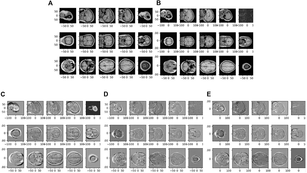
FIGURE 1. (A, B): One example pair of neuroimages used for registration, shown using 5 slices in each of the sagittal (top row) coronal (middle row) and axial (bottom row) planes. Difference between atlas and target images is shown before registration in (C), after affine registration in (D), and after rigid registration in (E).

We compare the natural gradient descent approach described here to three different gradient descent approaches. In the “vanilla” method we update the linear and translation jointly with no scaling, and in the “alternating” method we update them every other iteration (i.e., we update the linear part on iteration 0, the translation part on iteration one, the linear part on iteration 2, etc.).

We also compare to one other approach, “automatic scales estimation” used in simple elastix [22]. In this approach, the derivative of the transformation’s output with respect to each parameter is taken, yielding a 3 × 12 matrix of partial derivatives at each pixel. Next the sum of squares is computed down each row, yielding a 1 × 12 vector at each pixel. Last the quantity is averaged over all pixels. This gives a set of scale factors which are used to normalize the components of the gradient before updating parameters. These scale factors are generally only computed once. We note that this is related to our approach with three modifications: 1) we set I(x) = x in Eq. 3, 2) we consider the diagonal elements of g only, and 3) we define the components of g_A to be equal to those of g_id.

In all cases, gradient update steps are performed using a golden section linesearch with a maximum of 10 steps. The minimum in a given search direction is bracketed by a step size of 0, and a step size that would increase the loss. The latter is found by increasing the stepsize found from the previous iteration by a the golden ratio (roughly 1.6) until the loss function increases. Occasionally the step size is found from the golden section search to be 0 within machine precision, in which case we set it to 1 × 10^–10 to initialize the procedure at the next gradient descent iteration. Note that in this case optimization will stop, except in the alternating method where it may continue.

For each gradient descent method we consider 12 parameter affine registration (for sum of square error and mutual information loss), and 6 parameter rigid registration (sum of square error only). We also consider placements of the coordinate origin in the image center, half way to the corner, and at the corner. For one case we consider a finer grained sampling of the image origin as discussed in the results section.

In each case we compute the loss function at each step of optimization for 50 steps, and report normalized results that have been shifted and scaled to lie in the range 0–1. The minimum for the best method is assigned the value 0, and the initial value of the loss function (equal for all methods) is assigned the value 1. We show these curves directly, and also show the average tied rank at each iteration. The tied rank for method X is defined as 1 plus the number of other methods X does better than, plus half of the number of other methods it performs equal to. This gives a number between 1 (worst) and 4 (best).

Algorithms are implemented in pytorch and gradients with respect to parameters are computed automatically. We use double precision arithmetic to deal with a large dynamic range of step sizes. For metric computation derivatives DI are computed on a voxel grid via centered differences, and integrals are computed by summing over voxels and multiplying by the voxel volume. Algorithms are run on a NVIDIA GeForce RTX 2080 Ti Rev. A GPU device with 11GB of memory.

3 Results

3.1 Methods Summary

In the methods section we derived a metric based on the L² norm of optical flow of a template image, for the 12 parameter affine and 6 parameter rigid case, and proposed a corresponding natural gradient optimization algorithm. These correspond to 12 × 12 or 6 × 6 (respectively) positive definite matrices that depend on an atlas image.

We test our approach using 100 randomly selected pairs of neuroimages from the LPBA 40 dataset [5]. We consider four methods (natural gradient descent, “vanilla” gradient descent, alternating minimization, and automatic scales estimation), 3 placements of coordinate origins (center, half way, and corner), 2 transformation groups (affine and rigid), and 2 loss functions (sum of square error, and mutual information used in the 12 parameter case only).

Our first randomly selected pair of images is shown in Figures 1A,B. We also show the initial error (difference between images) in Figure 1C, and the error after alignment for the affine Figure 1D and rigid Figure 1E case.

3.2 Metric Tensors

For the example images in Figure 1, the metric tensor at identity for the 12 parameter affine registration is shown in Figure 2. The three plots show results when the origin is at the center, half way to the corner, and at the corner. Even with the origin in the center, the tensor has significant off diagonal elements, including negative values, suggesting that simply scaling gradient components is suboptimal. With the origin at the corner, there are stronger off diagonal elements, and a much larger difference between the linear and translation parts.

FIGURE 2

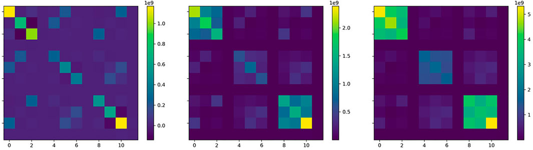
FIGURE 2. Metric tensors shown here for 12 parameter affine transformations. Left: origin at the center, middle: origin half way, right: origin at the corner.

For the example images in Figure 1, the metric tensor at identity for the 6 parameter rigid registration is shown in Figure 3. Similar trends are observed, with even stronger negative elements.

FIGURE 3

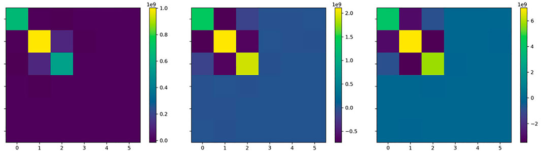
FIGURE 3. Metric tensors shown here for 6 parameter rigid transformations. Left: origin at the center, middle: origin half way, right: origin at the corner.

3.3 12 Parameter Affine Results With Sum of Square Error

Normalized sum of square error is reported as a function of optimization step in Figure 4 for the 12 parameter affine registrations. The median for each method is shown as a solid line, the 25th and 75th percentile are shown as a filled area, and all 100 curves are shown in pale colors. One observes that the natural gradient descent approach converges significantly faster than the other methods. Considering different coordinate origins has a large effect for the alternative methods and no effect for the natural gradient method. The alternative methods often fail to converge within 50 iterations, with the “vanilla” method failing even with a centered coordinate origin. This illustrates the important lack of robustness in this field.

FIGURE 4

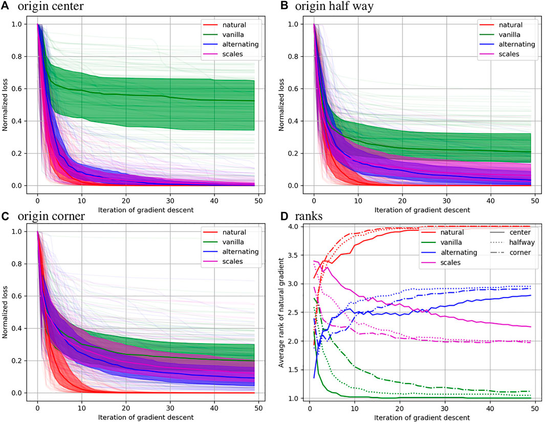
FIGURE 4. Results of minimizing sum of square error over 12 parameter affine registrations are shown with the coordinate origin in the center (A), half way to the corner (B), and in the corner (C). In these plots the normalized value of the objective function is shown at each iteration of gradient based optimization. In (D) the rank of each method is shown under each of these conditions.

The bottom right plot shows that the natural gradient method quickly achieves an average rank close to 4 (best), while the vanilla method quickly achieves a rank of 1 (worst). The alternating minimization approach performs better in the long term, while the automatic scales estimation approach performs better in the short term. Relative to the other methods our approach performs worse with a coordinate origin in the center and slightly better for a coordinate origin in the corner, though the effect is minor.

3.4 12 Parameter Affine Results With Mutual Information

Mutual information is reported as a function of optimization step in Figure 5 for the 12 parameter affine registrations. The median for each method is shown as a solid line, the 25th and 75th percentile are shown as a filled area, and all 100 curves are shown in pale colors. Trends are very similar to that seen for sum of square error, with the natural gradient descent method converging to the best even more quickly than for sum of square error.

FIGURE 5

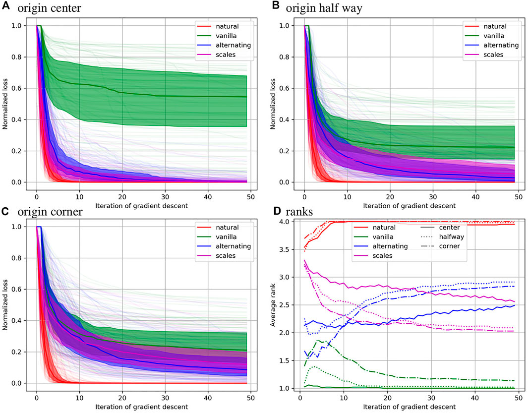
FIGURE 5. Results of minimizing negative mutual information 12 parameter affine registrations are shown with the coordinate origin in the center (A), half way to the corner (B), and in the corner (C). In these plots the normalized value of the objective function is shown at each iteration of gradient based optimization. In (D) the rank of each method is shown under each of these conditions.

3.5 6 Parameter Rigid Results With Sum of Square Error

Normalized sum of square error is reported as a function of optimization step in Figure 6 for the 6 parameter rigid registrations. The median for each method is shown as a solid line, the 25th and 75th percentile are shown as a filled area, and all 100 curves are shown in pale colors. One observes that the natural gradient descent approach converges significantly faster than the other methods for every origin placement except the center. Again, considering different coordinate origins has a large effect for the alternative methods and no effect for the natural gradient method.

FIGURE 6

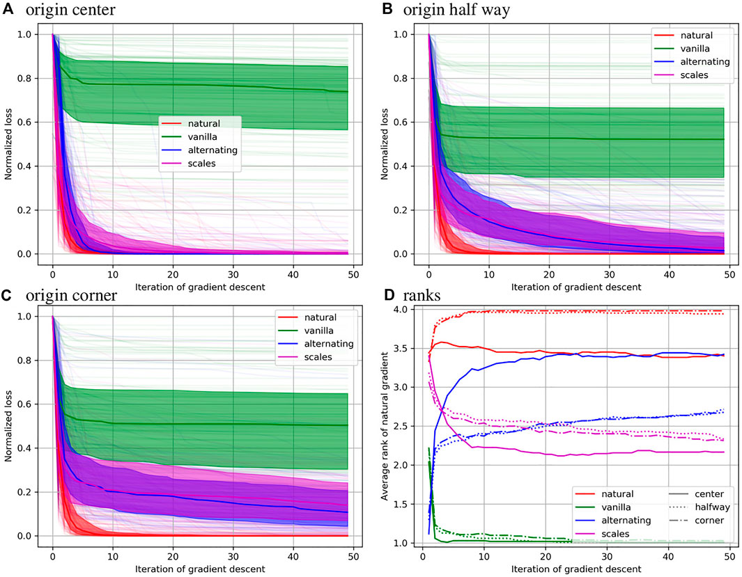
FIGURE 6. Results of minimizing sum of square error over 6 parameter rigid registrations are shown with the coordinate origin in the center (A), half way to the corner (B), and in the corner (C). In these plots the normalized value of the objective function is shown at each iteration of gradient based optimization. In (D) the rank of each method is shown under each of these conditions.

The bottom right plot shows that the natural gradient method quickly achieves an average rank close to 4 (best) for every case except a centered origin, where it tends to perform roughly equivalent to the alternating minimization scheme. The vanilla method quickly achieves a rank of 1 (worst). The alternating minimization approach performs better in the long term, while the automatic scales estimation approach performs better in the short term, although the order changes much sooner than in the 12 parameter case. Relative to the other methods, our approach performs worse with a coordinate origin in the center, and slightly better for a coordinate origin in the corner.

Because of the similarity between the alternating and natural gradient methods when the origin is centered, we consider comparing these methods as a function of origin position. We consider fraction between center and corner of 0, 0.1, 0.2, 0.3, 0.4, 0.5, and 1. For each iteration, and for each distance from the center, we use a sign test statistic by averaging across patients. Because this amounts to 350 statistical tests, we control familywise error rate using permutation testing [27]. We randomly flip the sign of each patient 100,000 times, and calculate corrected p values using maximum statistics. These results are shown in Figure 7. We see that the natural gradient method performs statistically significantly better than the alternating optimization method across all iterations when the origin is shifted by 0.2 or more, and for the first few iterations when the origin is shifted by 0.1 or less. This indicates that even small uncertainties in positioning of the origin, 3.6 cm in this case, can degrade the performance of traditional approaches. Shifts of this size are reasonable considering that the location of the brain’s center is typically unknown until after this type of registration is performed.

FIGURE 7

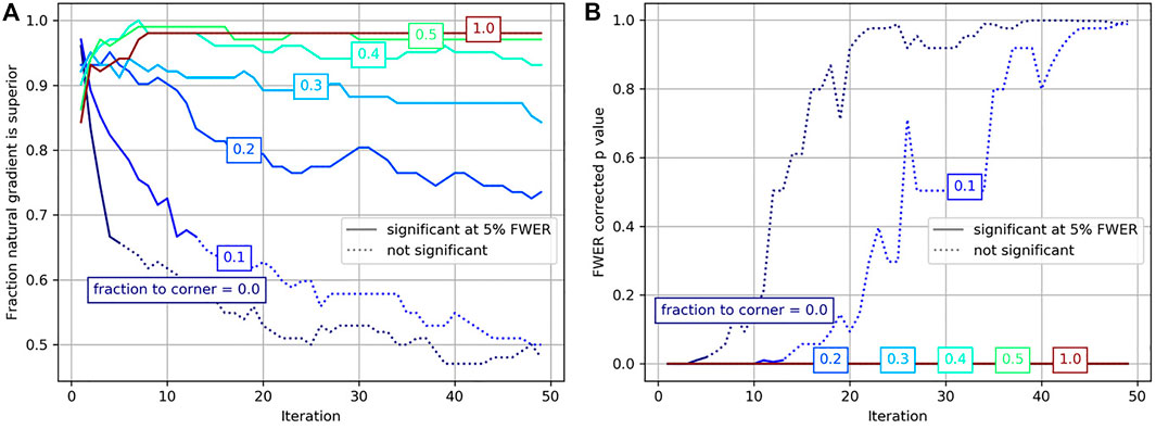
FIGURE 7. Comparison between the alternating minimization and natural gradient method are shown at each iteration of optimization for coordinate origin placed at various fractions of the distance between the center and the corner. (A) shows the fraction of the time the natural gradient method performs the best, with statistically significant (familywise error rate corrected p values less than 0.05) samples shown as solid lines. (B) shows the familywise error rate p values under the same conditions.

4 Discussion

Our results show that the natural gradient method proposed here outperforms other gradient based minimization schemes in almost every case examined, with virtually no computational overhead. This result holds for both 12 parameter affine transformations and 6 parameter rigid transformations, for sum of square error and for mutual information objective functions. The method does not depend on the placement of the coordinate origin, and can be easily implemented within any registration framework to improve convergence speed and reduce the number of hyperparameters that need to be tuned or estimated.

Another interesting finding is that the automatic scales estimation approach, while sophisticated, tends to perform worse than the simpler alternating minimization approach. This is particularly true when the origin is centered, which is the setting recommended by simple elastix [22].

There are few studies of natural gradient descent applied to image registration in the literature. A search on google scholar for “natural gradient” image registration returns only two relevant results. The work [28] uses a Fisher information metric for deformable registration and adopts various sampling strategies to define a random process from which it can be computed. The work [29] uses a similar strategy for deformable registration, but considers pairwise registration in a population and therefore computes a Fisher Information metric by taking an expectation across the population. Both rely on some form of stochasticity, and neither of these consider or exploit invariance with respect to a transformation group. In [15], which considers nonlinear registration (Large Deformation Diffeomorphic Image Mapping, LDDMM), a distinction between covectors and vectors in the space of smooth vector fields is made, and gradient descent is performed in the latter by applying a smoothing operation which is equivalent to the inverse of a metric. Other deformable registration approaches with regularization may do this implicitly. This right invariant metric used in LDDMM does not depend on the images being registered, and is based on spatial smoothness which is not relevant in the affine registration case. In related work [30, 31] developed strategies to learn a metric for deformable image registration, but considered these choices from an accuracy point of view rather than an optimization point of view. In this deformable registration setting, Gauss Newton optimization was used in [32], which is similar to our approach as described in Section 2.5.2.

The trend in computer vision and deep learning is to use stochastic gradient descent methods for optimization, and ITK and its derivatives includes several of these approaches for image registration. For example, the work of [33–35] is used for adaptive stepsize estimation. Other adaptive step size approaches have been developed and applied to deformable image registration as well [36]. These approaches do not consider different scale factors for different parameters. The well known ADAM optimization procedure [37] does update step sizes on a per parameter basis, but does not allow for mixing of parameters. The importance of this mixing is evident from the significant off diagonal elements seen in Figures 2, 3.

A modern trend in image registration is to use deep learning based approaches that replace optimization procedures considered here with prediction using a single forward pass of a deep network. These tools include Voxelmorph [38], Quicksilver [39], and others. While our contribution here does not apply directly to these methods, it could potentially be used to accelerate the training stage. An investigation into this potential will be the subject of future work.

Finally, the simple registration tasks considered here are often only one step in a long pipeline or joint optimization procedure. For example, in our work studying serial section images, 3D affine registration is performed jointly with nonlinear alignment and 2D rigid registration on each slice [40, 41]. The approach developed here leads to a reduction by half in the number of parameters that need to be selected manually, allowing our pipeline to generalize to new datasets more effectively. This work demonstrates that straightforward applications of principles from differential geometry can accelerate research in neuroimaging.

Data Availability Statement

Publicly available datasets were analyzed in this study. This data can be found here: Laboratory of Neuroimaging LPBA40 atlas repository https://www.loni.usc.edu/research/atlases.

Author Contributions

DT conceived of the study, developed the methods, carried out the analysis, and wrote the manuscript.

Funding

This work was supported by the National Institutes of Health (U19MH114821), and the Karen Toffler Charitable Trust through the Toffler Scholar Program.

Conflict of Interest

The author declares that the research was conducted in the absence of any commercial or financial relationships that could be construed as a potential conflict of interest.

Publisher’s Note

All claims expressed in this article are solely those of the authors and do not necessarily represent those of their affiliated organizations, or those of the publisher, the editors and the reviewers. Any product that may be evaluated in this article, or claim that may be made by its manufacturer, is not guaranteed or endorsed by the publisher.

References

1. Jack, CR, Bernstein, MA, Fox, NC, Thompson, P, Alexander, G, Harvey, D, et al. The Alzheimer's Disease Neuroimaging Initiative (ADNI): MRI Methods. J Magn Reson Imaging (2008) 27:685–91. doi:10.1002/jmri.21049

PubMed Abstract | CrossRef Full Text | Google Scholar

2. Marcus, DS, Wang, TH, Parker, J, Csernansky, JG, Morris, JC, and Buckner, RL. Open Access Series of Imaging Studies (Oasis): Cross-Sectional Mri Data in Young, Middle Aged, Nondemented, and Demented Older Adults. J Cogn Neurosci (2007) 19:1498–507. doi:10.1162/jocn.2007.19.9.1498

PubMed Abstract | CrossRef Full Text | Google Scholar

3. Benninger, K, Hood, G, Simmel, D, Tuite, L, Wetzel, A, Ropelewski, A, et al. Cyberinfrastructure of a Multi-Petabyte Microscopy Resource for Neuroscience Research. In: Practice and Experience in Advanced Research Computing, Portland, OR, July 26–30, 2020 (2020). p. 1–7. doi:10.1145/3311790.3396653

CrossRef Full Text | Google Scholar

4. Fonov, V, Evans, A, McKinstry, R, Almli, C, and Collins, D. Unbiased Nonlinear Average Age-Appropriate Brain Templates from Birth to Adulthood. NeuroImage (2009) 47:S102. doi:10.1016/s1053-8119(09)70884-5

CrossRef Full Text | Google Scholar

5. Shattuck, DW, Mirza, M, Adisetiyo, V, Hojatkashani, C, Salamon, G, Narr, KL, et al. Construction of a 3d Probabilistic Atlas of Human Cortical Structures. Neuroimage (2008) 39:1064–80. doi:10.1016/j.neuroimage.2007.09.031

PubMed Abstract | CrossRef Full Text | Google Scholar

6. Wang, Q, Ding, S-L, Li, Y, Royall, J, Feng, D, Lesnar, P, et al. The allen Mouse Brain Common Coordinate Framework: a 3d Reference Atlas. Cell (2020) 181:936–53. doi:10.1016/j.cell.2020.04.007

PubMed Abstract | CrossRef Full Text | Google Scholar

7. Bookstein, FL. Morphometric Tools for Landmark Data: Geometry and Biology. Cambridge, United Kingdom: Cambridge University Press (1997).

8. Joshi, SC, and Miller, MI. Landmark Matching via Large Deformation Diffeomorphisms. IEEE Trans Image Process (2000) 9:1357–70. doi:10.1109/83.855431

PubMed Abstract | CrossRef Full Text | Google Scholar

9. Miller, MI, Tward, DJ, and Trouvé, A. Coarse-to-fine Hamiltonian Dynamics of Hierarchical Flows in Computational Anatomy. In: Proceedings of the IEEE/CVF Conference on Computer Vision and Pattern Recognition Workshops, Seattle, WA, June 14–19, 2020 (2020). p. 860–1. doi:10.1109/cvprw50498.2020.00438

CrossRef Full Text | Google Scholar

10. Glaunès, J, Qiu, A, Miller, MI, and Younes, L. Large Deformation Diffeomorphic Metric Curve Mapping. Int J Comput Vis (2008) 80:317–36. doi:10.1007/s11263-008-0141-9

PubMed Abstract | CrossRef Full Text | Google Scholar

11. Vaillant, M, and Glaunès, J. Surface Matching via Currents. In: Biennial International Conference on Information Processing in Medical Imaging, Glenwood Springs, CO, July 10–15, 2005. Springer (2005). p. 381–92. doi:10.1007/11505730_32

CrossRef Full Text | Google Scholar

12. Charon, N, and Trouvé, A. The Varifold Representation of Nonoriented Shapes for Diffeomorphic Registration. SIAM J Imaging Sci (2013) 6:2547–80. doi:10.1137/130918885

CrossRef Full Text | Google Scholar

13. Woods, RP, Grafton, ST, Holmes, CJ, Cherry, SR, and Mazziotta, JC. Automated Image Registration: I. General Methods and Intrasubject, Intramodality Validation. J Comput Assist tomogr (1998) 22:139–52. doi:10.1097/00004728-199801000-00027

PubMed Abstract | CrossRef Full Text | Google Scholar

14. Woods, RP, Grafton, ST, Watson, JDG, Sicotte, NL, and Mazziotta, JC. Automated Image Registration: Ii. Intersubject Validation of Linear and Nonlinear Models. J Comput Assist tomogr (1998) 22:153–65. doi:10.1097/00004728-199801000-00028

PubMed Abstract | CrossRef Full Text | Google Scholar

15. Beg, MF, Miller, MI, Trouvé, A, and Younes, L. Computing Large Deformation Metric Mappings via Geodesic Flows of Diffeomorphisms. Int J Comput Vis (2005) 61:139–57. doi:10.1023/b:visi.0000043755.93987.aa

CrossRef Full Text | Google Scholar

16. Reuter, M, Rosas, HD, and Fischl, B. Highly Accurate Inverse Consistent Registration: a Robust Approach. Neuroimage (2010) 53:1181–96. doi:10.1016/j.neuroimage.2010.07.020

PubMed Abstract | CrossRef Full Text | Google Scholar

17. Tward, D, Brown, T, Kageyama, Y, Patel, J, Hou, Z, Mori, S, et al. Diffeomorphic Registration with Intensity Transformation and Missing Data: Application to 3D Digital Pathology of Alzheimer's Disease. Front Neurosci (2020) 14:52. doi:10.3389/fnins.2020.00052

PubMed Abstract | CrossRef Full Text | Google Scholar

18. Joshi, AA, Shattuck, DW, Thompson, PM, and Leahy, RM. Surface-constrained Volumetric Brain Registration Using Harmonic Mappings. IEEE Trans Med Imaging (2007) 26:1657–69. doi:10.1109/tmi.2007.901432

PubMed Abstract | CrossRef Full Text | Google Scholar

19. Durrleman, S, Prastawa, M, Korenberg, JR, Joshi, S, Trouvé, A, and Gerig, G. Topology Preserving Atlas Construction from Shape Data without Correspondence Using Sparse Parameters. In: International Conference on Medical Image Computing and Computer-Assisted Intervention, Nice, France, October 1–5, 2012. Springer (2012). p. 223–30. doi:10.1007/978-3-642-33454-2_28

CrossRef Full Text | Google Scholar

20. Tward, D, Miller, M, Trouve, A, and Younes, L. Parametric Surface Diffeomorphometry for Low Dimensional Embeddings of Dense Segmentations and Imagery. IEEE Trans Pattern Anal Mach Intell (2016) 39:1195–208. doi:10.1109/TPAMI.2016.2578317

PubMed Abstract | CrossRef Full Text | Google Scholar

21. Klein, A, Andersson, J, Ardekani, BA, Ashburner, J, Avants, B, Chiang, M-C, et al. Evaluation of 14 Nonlinear Deformation Algorithms Applied to Human Brain Mri Registration. Neuroimage (2009) 46:786–802. doi:10.1016/j.neuroimage.2008.12.037

PubMed Abstract | CrossRef Full Text | Google Scholar

22. Marstal, K, Berendsen, F, Staring, M, and Klein, S. Simpleelastix: A User-Friendly, Multi-Lingual Library for Medical Image Registration. In: Proceedings of the IEEE conference on computer vision and pattern recognition workshops, Las Vegas, NV, June 26–July 1, 2016 (2016). p. 134–42. doi:10.1109/cvprw.2016.78

CrossRef Full Text | Google Scholar

23. Yaniv, Z, Lowekamp, BC, Johnson, HJ, and Beare, R. Simpleitk Image-Analysis Notebooks: a Collaborative Environment for Education and Reproducible Research. J Digit Imaging (2018) 31:290–303. doi:10.1007/s10278-017-0037-8

PubMed Abstract | CrossRef Full Text | Google Scholar

24. McCormick, M, Liu, X, Jomier, J, Marion, C, and Ibanez, L. Itk: Enabling Reproducible Research and Open Science. Front Neuroinform (2014) 8:13. doi:10.3389/fninf.2014.00013

PubMed Abstract | CrossRef Full Text | Google Scholar

25. Yoo, TS, Ackerman, MJ, Lorensen, WE, Schroeder, W, Chalana, V, Aylward, S, et al. Engineering and Algorithm Design for an Image Processing API: a Technical Report on ITK-Tthe Insight Toolkit. Stud Health Technol Inform (2002) 85:586–92. doi:10.3233/978-1-60750-929-5-586

PubMed Abstract | Google Scholar

26. Amari, SI, and Douglas, SC. In: Why natural gradient? Proceedings of the 1998 IEEE International Conference on Acoustics, Speech and Signal Processing, ICASSP’98 (Cat. No. 98CH36181), Seatle, WA, May 15, 1998, 2. IEEE (1998). p. 1213–6.

27. Nichols, T, and Hayasaka, S. Controlling the Familywise Error Rate in Functional Neuroimaging: a Comparative Review. Stat Methods Med Res (2003) 12:419–46. doi:10.1191/0962280203sm341ra

PubMed Abstract | CrossRef Full Text | Google Scholar

28. Zikic, D, Kamen, A, and Navab, N. Natural Gradients for Deformable Registration. In: 2010 IEEE Computer Society Conference on Computer Vision and Pattern Recognition, San Francisco, CA, June 15–17, 2010. IEEE (2010). p. 2847–54. doi:10.1109/cvpr.2010.5540019

CrossRef Full Text | Google Scholar

29. Wang, H, Rusu, M, Golden, T, Gow, A, and Madabhushi, A. Mouse Lung Volume Reconstruction from Efficient Groupwise Registration of Individual Histological Slices with Natural Gradient. In: Medical Imaging 2013: Image Processing, Lake Buena, FL, February 9–14, 2013, 8669. Bellingham, WA: International Society for Optics and Photonics (2013). p. 866914. doi:10.1117/12.2006860

CrossRef Full Text | Google Scholar

30. Vialard, F-X, and Risser, L. Spatially-varying Metric Learning for Diffeomorphic Image Registration: A Variational Framework. In: International Conference on Medical Image Computing and Computer-Assisted Intervention, Boston, MA, September 14–18, 2014. Springer (2014). p. 227–34. doi:10.1007/978-3-319-10404-1_29

CrossRef Full Text | Google Scholar

31. Niethammer, M, Kwitt, R, and Vialard, FX. Metric Learning for Image Registration. In: Proceedings of the IEEE Conference on Computer Vision and Pattern Recognition, Long Beach, CA, June 16–20, 2019, 2019 (2019). p. 8455–64. doi:10.1109/cvpr.2019.00866

PubMed Abstract | CrossRef Full Text | Google Scholar

32. Ashburner, J, and Friston, KJ. Diffeomorphic Registration Using Geodesic Shooting and Gauss-Newton Optimisation. NeuroImage (2011) 55:954–67. doi:10.1016/j.neuroimage.2010.12.049

PubMed Abstract | CrossRef Full Text | Google Scholar

33. Klein, S, Pluim, JPW, Staring, M, and Viergever, MA. Adaptive Stochastic Gradient Descent Optimisation for Image Registration. Int J Comput Vis (2009) 81:227–39. doi:10.1007/s11263-008-0168-y

CrossRef Full Text | Google Scholar

34. Qiao, Y, Lelieveldt, BPF, and Staring, M. An Efficient Preconditioner for Stochastic Gradient Descent Optimization of Image Registration. IEEE Trans Med Imaging (2019) 38:2314–25. doi:10.1109/tmi.2019.2897943

PubMed Abstract | CrossRef Full Text | Google Scholar

35. Cruz, P. Almost Sure Convergence and Asymptotical Normality of a Generalization of Kesten’s Stochastic Approximation Algorithm for Multidimensional Case. arXiv preprint arXiv:1105.5231 (2011).

Google Scholar

36. Wu, J, and Tang, X. A Large Deformation Diffeomorphic Framework for Fast Brain Image Registration via Parallel Computing and Optimization. Neuroinformatics (2020) 18 (2), 251–266. doi:10.1007/s12021-019-09438-7

CrossRef Full Text | Google Scholar

37. Kingma, DP, and Ba, J. Adam: A Method for Stochastic Optimization. In International Conference on Learning Representations 2013, San Diego, CA, May 7–9, 2015 (2015).

Google Scholar

38. Balakrishnan, G, Zhao, A, Sabuncu, MR, Guttag, J, and Dalca, AV. Voxelmorph: a Learning Framework for Deformable Medical Image Registration. IEEE Trans Med Imaging (2019) 38:1788–800. doi:10.1109/tmi.2019.2897538

PubMed Abstract | CrossRef Full Text | Google Scholar

39. Yang, X, Kwitt, R, Styner, M, and Niethammer, M. Quicksilver: Fast Predictive Image Registration - A Deep Learning Approach. NeuroImage (2017) 158:378–96. doi:10.1016/j.neuroimage.2017.07.008

PubMed Abstract | CrossRef Full Text | Google Scholar

40. Tward, DJ, Li, X, Huo, B, Lee, BC, Miller, M, and Mitra, PP. Solving the where Problem in Neuroanatomy: A Generative Framework with Learned Mappings to Register Multimodal, Incomplete Data into a Reference Brain. Cold Spring Harbor, NY: bioRxiv (2020).

41. Tward, D, Li, X, Huo, B, Lee, B, Mitra, P, and Miller, M. 3d Mapping of Serial Histology Sections with Anomalies Using a Novel Robust Deformable Registration Algorithm. In: 7th International Workshop on Mathematical Foundations of Computational Anatomy, Held in Conjunction with MICCAI 2019, Shenzhen, China, October 17, 2019. Springer (2019). p. 162–73. doi:10.1007/978-3-030-33226-6_18

CrossRef Full Text | Google Scholar