 Michael Götte
 Reinhold Schneider
 Philipp Trunschke
- Department of Mathematics, Technische Universität Berlin, Berlin, Germany
Low-rank tensors are an established framework for the parametrization of multivariate polynomials. We propose to extend this framework by including the concept of block-sparsity to efficiently parametrize homogeneous, multivariate polynomials with low-rank tensors. This provides a representation of general multivariate polynomials as a sum of homogeneous, multivariate polynomials, represented by block-sparse, low-rank tensors. We show that this sum can be concisely represented by a single block-sparse, low-rank tensor.
We further prove cases, where low-rank tensors are particularly well suited by showing that for banded symmetric tensors of homogeneous polynomials the block sizes in the block-sparse multivariate polynomial space can be bounded independent of the number of variables.
We showcase this format by applying it to high-dimensional least squares regression problems where it demonstrates improved computational resource utilization and sample efficiency.
1 Introduction
An important problem in many applications is the identification of a function from measurements or random samples. For this problem to be well-posed, some prior information about the function has to be assumed and a common requirement is that the function can be approximated in a finite dimensional ansatz space. For the purpose of extracting governing equations the most famous approach in recent years has been SINDy [1]. However, the applicability of SINDy to high-dimensional problems is limited since truly high-dimensional problems require a nonlinear parameterization of the ansatz space. One particular reparametrization that has proven itself in many applications are tensor networks. These allow for a straight-forward extension of SINDy [2] but can also encode additional structure as presented in [3]. The compressive capabilities of tensor networks originate from this ability to exploit additional structure like smoothness, locality or self-similarity and have hence been used in solving high-dimensional equations [4–7]. In the context of optimal control tensor train networks have been utilized for solving the Hamilton–Jacobi–Bellman equation in [8,9], for solving backward stochastic differential equations in [10] and for the calculation of stock options prices in [11,12]. In the context of uncertainty quantification they are used in [13–15] and in the context of image classification they are used in [16,17].
A common thread in these publications is the parametrization of a high-dimensional ansatz space by a tensor train network which is then optimized. In most cases this means that the least-squares error of the parametrized function to the data is minimized. There exist many methods to perform this minimization. A well-known algorithm in the mathematics community is the alternating least-squares (ALS) [18,19], which is related to the famous DMRG method [20] for solving the Schrödinger equation in quantum physics. Although, not directly suitable for recovery tasks, it became apparent that DMRG and ALS can be adapted to work in this context. Two of these extensions to the ALS algorithm are the stablilized ALS approximation (SALSA) [21] and the block alternating steepest descent for Recovery (bASD) algorithm [13]. Both adapt the tensor network ranks and are better suited to the problem of data identification. Since the set of tensor trains of fixed rank forms a manifold [22] it is also possible to perform gradient based optimization schemes [48]. This however is not a path that we pursue in this work. Our contribution extends the ALS (and SALSA) algorithm and we believe that it can be applied to many of the fields stated above.
In this work we consider ansatz spaces of homogeneous polynomials of fixed degree and their extension to polynomials of bounded degree. We introduce the concept of block-sparsity as an efficient way to parametrize homogeneous polynomials with low rank tensors. Although, this is not the first instance in which sparsity is used in the context of low-rank tensors (see [24–26]), we believe, that this is the first time where block-sparsity is used to parametrize homogeneous polynomials. The sparsity used in the previous works is substantially different to the block-sparsity discussed in this work. Block-sparsity is preserved under most tensor network operations such as summation, orthogonalization and rounding and the parametrization of tangent spaces which is not the case for standard sparsity. This is important since orthogonalization is an essential part of numerically stable and efficient optimization schemes and means that most of the existing tensor methods, like HSVD (see [27]), ALS, SALSA or Riemannian optimization can be performed in this format. We also show that, if the symmetric tensor of a homogeneous polynomial is banded, it can be represented very efficiently in the tensor train format, since the sizes of the non-zero blocks can be bounded independently of the number of variables. In physics this property can be associated with the property of locality, which can be used to identify cases where tensor trains work exceptionally well.
Quantum physicists have used the concept of block-sparsity for at least a decade [28] but it was introduced to the mathematics community only recently in [29]. In the language of quantum mechanics one would say that there exists an operator for which the coefficient tensor of any homogeneous polynomial is an eigenvector. This encodes a symmetry, where the eigenvalue of this eigenvector is the degree of the homogeneous polynomial, which acts as a quantum number and corresponds to the particle number of bosons and fermions.
The presented approach is very versatile and can be combined with many polynomial approximation strategies like the use of Taylor’s theorem in [30] and there exist many approximation theoretic results that ensure a good approximation with a low degree polynomial for many classes of functions (see e.g. [31]).
In addition to the approximation theoretic results, we can motivate these polynomial spaces by thinking about the sample complexity for successful recovery in the case of regression problems. In [32] it was shown that for tensor networks the sample complexity, meaning the number of data points needed, is related to the dimension of the high-dimensional ansatz space. But, these huge sample sizes are not needed in most practical examples [14]. This suggests that the regularity of the sought function must have a strong influence on the number of samples that are required. However, for most practical applications, suitable regularity guarantees cannot be made — neither for the best approximation nor for the initial guess, nor any iterate of the optimization process. By restricting ourselves to spaces of homogeneous polynomials, the gap between observed sample complexity and proven worst-case bound is reduced.
In the regression setting, this means that we kill two birds with one stone. By applying block-sparsity to the coefficient tensor we can restrict the ansatz space to well-behaved functions which can be identified with a reasonable sample size. At the same time we reduce the number of parameters and speed up the least-squares minimization task. Finally, note that this parametrization allows practitioners to devise algorithms that are adaptive in the degree of the polynomial, thereby increasing the computational resource utilization even further. This solves a real problem in practical applications where the additional and unnecessary degrees of freedom of conventional low-rank tensor formats cause many optimization algorithms to get stuck in local minima.
The remainder of this work is structured as follows. Notation introduces basic tensor notation, the different parametrizations of polynomials that are used in this work and then formulates the associated least-squares problems. In Theoretical Foundation we state the known results on sampling complexity and block sparsity. Furthermore, we set the two results in relation and argue why this leads to more favorable ansatz spaces. This includes a proof of rank-bounds for a class of homogeneous polynomials which can be represented particularly efficient as tensor trains. Method Description derives two parametrizations from the results of Theoretical Foundation and presents the algorithms that are used to solve the associated least-squares problems. Finally, Numerical Results gives some numerical results for different classes of problems focusing on the comparison of the sample complexity for the full- and sub-spaces. Most notably, the recovery of a quantity of interest for a parametric PDE, where our approach achieves successful recovery with relatively few parameters and samples. We observed that for suitable problems the number of parameters can be reduced by a factor of almost 10.
2 Notation
In our opinion, using a graphical notation for the involved contractions in a tensor network drastically simplifies the expressions making the whole setup more approachable. This section introduces this graphical notation for tensor networks, the spaces that will be used in the remainder of this work and the regression framework.
2.1 Tensors and Indices
Definition 2.1. Let
To define further operations on tensors it is often useful to associate each mode with a symbolic index.
Definition 2.2. A symbolic indexi of dimension n is a placeholder for an arbitrary but fixed natural number between 1 and n. For a dimension tuple n of order d and a tensor
where
Remark 2.3. We use the letters i and j (with appropriate subscripts) for symbolic indices while reserving the letters k, l and m for ordinary indices.
Example 2.4. Let x be an order 2 tensor with mode dimensions n1 and n2, i.e. an n1-by-n2 matrix. Then x (ℓ1, j) denotes the ℓ1-th row of x and x (i, ℓ2) denotes the ℓ2-th column of x.
Inspired by Einstein notation we use the concept of symbolic indices to define different operations on tensors.
Definition 2.5. Let i1 and i2 be (symbolic) indices of dimension n1 and n2, respectively and let φ be a bijection
We then define the product of indices with respect to φ as j = φ(i1, i2) where j is a (symbolic) index of dimension n1n2. In most cases the choice of bijection is not important and we will write i1 ⋅ i2≔φ(i1, i2) for an arbitrary but fixed bijection φ. For a tensor x of dimension (n1, n2) the expression
defines the tensor y of dimension (n1n2) while the expression
defines
Definition 2.6. Consider the tensors
defines the tensor
defines the tensor
defines the tensor
We choose this description mainly because of its simplicity and how it relates to the implementation of these operations in the numeric libraries numpy [33] and xerus [34].
2.2 Graphical Notation and Tensor Networks
This section will introduce the concept of tensor networks [35] and a graphical notation for certain operations which will simplify working with these structures. To this end we reformulate the operations introduced in the last section in terms of nodes, edges and half-edges.
Definition 2.7. For a dimension tuple n of order d and a tensor 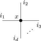 where the node represents the tensor and the half-edges represent the d different modes of the tensor illustrated by the symbolic indices i1, …, id.
With this definition we can write the reshapings of Defintion 2.5 simply as

and also simplify the binary operations of Definition 2.6.
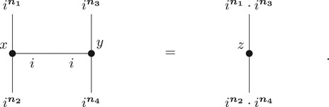
Definition 2.8. Let
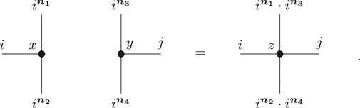
and defines
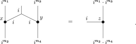
and defines
With these definitions we can compose entire networks of multiple tensors which are called tensor networks.
2.3 The Tensor Train Format
A prominent example of a tensor network is the tensor train (TT) [19,36], which is the main tensor network used throughout this work. This network is discussed in the following subsection.
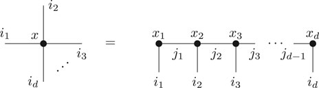
Definition 2.9. Let n be an dimensional tuple of order-d. The TT format decomposes an order d tensor
The tuple (r1, …, rd−1) is called the representation rank of this representation.
In graphical notation it looks like this.
Remark 2.10. Note that this representation is not unique. For any pair of matrices (A, B) that satisfies AB = Id we can replace xk by xk (i1, i2, j) ⋅ A (j, i3) and xk+1 by B (i1, j) ⋅ x (j, i2, i3) without changing the tensor x.
The representation rank of x is therefore dependent on the specific representation of x as a TT, hence the name. Analogous to the concept of matrix rank we can define a minimal necessary rank that is required to represent a tensor x in the TT format.
Definition 2.11. The tensor train rank of a tensor
of minimal rk’s such that the xk compose x.
In [[22], Theorem 1a] it is shown that the TT-rank can be computed by simple matrix operations. Namely, rk can be computed by joining the first k indices and the remaining d − k indices and computing the rank of the resulting matrix. At last, we need to introduce the concept of left and right orthogonality for the tensor train format.
Definition 2.12. Let
Similarly, we call a tensor
A tensor train is left orthogonal if all component tensors x1, …, xd−1 are left orthogonal. It is right orthogonal if all component tensors x2, …, xd are right orthogonal.
Lemma 2.1 [36].For every tensor
For technical purposes it is also useful to define the so-called interface tensors, which are based on left and right orthogonal decompositions.
Definition 2.13. Let x be a tensor train of order d with rank tuple r.
For every k = 1, …, d and ℓ = 1, …, rk, the ℓ-th left interface vector is given by
where x is assumed to be left orthogonal. The ℓ-th right interface vector is given by
where x is assumed to be right orthogonal.
2.4 Sets of Polynomials
In this section we specify the setup for our method and define the majority of the different sets of polynomials that are used. We start by defining dictionaries of one dimensional functions which we then use to construct the different sets of high-dimensional functions.
Definition 2.14. Let
Example 2.15. Two simple examples of a function dictionary that we use in this work are given by the monomial basis of dimension p, i.e.
and by the basis of the first p Legendre polynomials, i.e.
Using function dictionaries we can define the following high-dimensional space of multivariate functions. Let Ψ be a function dictionary of size
This means that every function
with a coefficient tensor
where the TT rank of the coefficient is bounded. Every
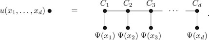
where the Ck’s are the components of the tensor train representation of the coefficient tensor
Remark 2.16. In this way every tensor
An important subspace of
where again ⟨•⟩ is the linear span. From this definition it is easy to see that a homogeneous polynomial of degree g can be represented as an element of
In Theoretical Foundation we will introduce an efficient representation of such coefficient tensors c in a block sparse tensor format.
Using
Based on this characterization we will define a block-sparse tensor train version of this space in Theoretical Foundation.
2.5 Parametrizing Homogeneous Polynomials by Symmetric Tensors
In algebraic geometry the space
where d = (d, …, d) is a dimension tuple of order g and
Since B is symmetric the sum simplifies to
From this follows that for
and δk,ℓ denotes the Kronecker delta. This demonstrates how our approach can alleviate the difficulties that arise when symmetric tensors are represented in the hierarchical tucker format [37] in a very simple fashion.
2.6 Least Squares
Let in the following
A practical problem that often arises when computing uW is that computing the L2(Ω)-norm is intractable for large d. Instead of using classical quadrature rules one often resorts to a Monte Carlo estimation of the high-dimensional integral. This means one draws M random samples
where ‖⋅‖F is the Frobenius norm. With this approximation we can define an empirical version of uW as
For a linear space W, computing uW,M amounts to solving a linear system and does not pose an algorithmic problem. We use the remainder of this section to comment on the minimization problem Eq. 14 when a set of tensor trains is used instead.
Given samples
Then the M-dimensional vector of evaluations of u at all given sample points is given by.
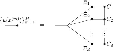 where we use Operation Eq. 2 to join the different M-dimensional indices.
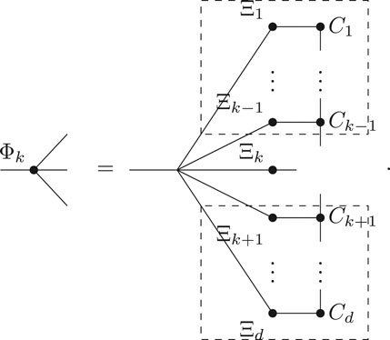
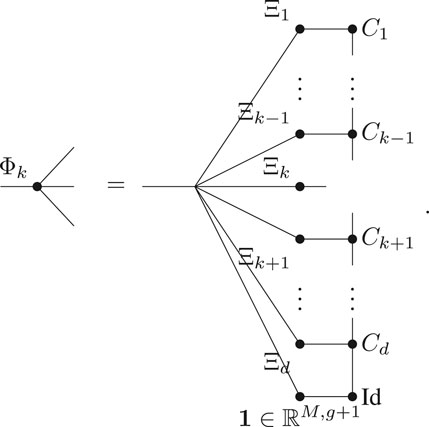
The alternating least-squares algorithm cyclically updates each component tensor Ck by minimizing the residual corresponding to this contraction. To formalize this we define the operator
 (16)
(16)
Then the update for Ck is given by a minimal residual solution of the linear system
where F(m)≔y(m)≔f (x(m)) and i1, i2, i3, j are symbolic indices of dimensions rk−1, nk, rk, M, respectively. The particular algorithm that is used for this minimization may be adapted to the problem at hand. These contractions are the basis for our algorithms in Method Description. We refer to [19] for more details on the ALS algorithm.
Note that it is possible to reuse parts of the contractions in Φk through so called stacks. In this way not the entire contraction has to be computed for every k. The dashed boxes mark the parts of the contraction that can be reused. Details on that can be found in [38].
3 Theoretical Foundation
3.1 Sample Complexity for Polynomials
The accuracy of the solution uW,M of Eq. 14 in relation to uW is subject to tremendous interest on the part of the mathematics community. Two particular papers that consider this problem are [32,39]. While the former provides sharper error bounds for the case of linear ansatz spaces the latter generalizes the work and is applicable to tensor network spaces. We now recall the relevant result for convenience.
Proposition 3.1.For any setW ⊆ L2(Ω) ∩ L∞(Ω), define the variation constant
Letδ ∈ (0, 2−1/2). IfWis a subset of a finite dimensional linear space andk≔ max{K ({f − uW}), K ({uW}− W)} < ∞it holds that
whereqdecreases exponentially with a rate of
Proof. Since k < ∞, Theorems 2.7 and 2.12 in [32] ensure that
holds with a probability of at least
Note that the value of k depends only on f and on the set W but not on the particular choice of representation of W. However, the variation constant of spaces like
by using techniques from [[32], Sample Complexity for Polynomials] and the fact that each Pℓ attains its maximum at 1. If
where the maximum is estimated by observing that (2 (ℓ1 + 1) − 1) (2ℓ2 − 1) ≤ (2ℓ1 − 1) (2 (ℓ2 + 1) − 1) ⇔ ℓ2 ≤ ℓ1. For g ≤ d this results in the simplified bound
In this work, we focus on the case where the samples are drawn according to a probability measure on Ω. This however is not a necessity and it is indeed beneficial to draw the samples from an adapted sampling measure. Doing so, the theory in [32] ensures that K(V) = dim(V) for all linear spaces V — independent of the underlying dictionary Ψ. This in turn leads to the bounds
3.2 Block Sparse Tensor Trains
Now that we have seen that it is advantageous to restrict ourselves to the space
This is the operator mentioned in the introduction encoding a quantum symmetry. In the context of quantum mechanics this operator is known as the bosonic particle number operator but we simply call it the degree operator. The reason for this is that for the function dictionary of monomials Ψmonomial the eigenspaces of L for eigenvalue g are associated with homogeneous polynomials of degreee g. Simply put, if the coefficient tensor c for the multivariate polynomial
for which we have
In the following we adopt the notation x = Lc to abbreviate the equation
where L is a tensor operator acting on a tensor c with result x.
Recall that by Remark 2.16 every TT corresponds to a polynomial by multiplying function dictionaries onto the cores. This means that for every ℓ = 1, …, r the TT
This is put rigorously in the first assertion in the subsequent Theorem 3.2. There
Theorem 3.2 [[29], Theorem 3.2]. Letp = (p, …, p) be a dimension tuple of sizedand
1. For all
for
2. The component tensors satisfy a block structure in the sets
where we set
Note that this generalizes to other dictionaries and is not restricted to monomials.
Although, block sparsity also appears for g + 1 ≠ p we restrict ourselves to the case g + 1 = p in this work. Note that then the eigenspace of L for the eigenvalue g has a dimension equal to the dimension of the space of homogeneous polynomials, namely
Lemma 3.3 [[29], Lemma 3.6]. Letp = (p, …, p) be a dimension tuple of sizedand
for allk = 1, …, d − 1 and
The proof of this lemma is based on a simple combinatorial argument. For every k consider the size of the groups
Example 3.1 (Block Sparsity). Let p = 4 and g = 3 be given and let c be a tensor train such that Lc = gc. Then for k = 2, …, d − 1 the component tensors Ck of c exhibit the following block sparsity (up to permutation). For indices i of order rk−1 and j of order rk
This block structure results from sorting the indices i and j in such a way that
The maximal block sizes
As one can see by Lemma 3.3 the block sizes
The expressive power of tensor train parametrizations can be understood by different concepts, such as locality or self similarity. We use the remainder of this section to provide d-independent rank bounds in the context of locality.
Definition 3.2. Let
Example 3.3. Let u be a homogeneous polynomial of degree 2 with variable locality Kloc. Then the symmetric matrix B (cf. Eq. 12) is Kloc-banded. For Kloc = 0 this means that B is diagonal and that u takes the form
This shows that variable locality removes mixed terms.
Remark 3.4. The locality condition in the following Theorem 3.4 is a sufficient, but in no way necessary, condition for a low rank. But since locality is a prominent feature of many physical phenomena, this condition allows us to identify an entire class of highly relevant functions which can be approximated very efficiently.
Consider, for example, a many-body system in one dimension, where each body is described by position and velocity coordinates. If the influence of neighboring bodies is much higher than the influence of more distant ones, the coefficients of the polynomial parts that depend on multiple variables often can be neglected. The forces in this system then exhibit a locality structure. An example of this is given in equation Eq. 6 in [3], where this structure is exhibited by the force that acts on the bodies. A similar structure also appears in the microscopic traffic models in Notation of [41].
Another example is given by the polynomial chaos expansion of the stochastic process
for
Theorem 3.4.Letp = (p, …, p) be a dimension tuple of sizedand
for allk = 1, …, d − 1 and
Proof. For fixed g > 0 and a fixed component Ck recall that for each l the tensor
This means that for ℓ = 1, …, Kloc each block Qℓ matches a polynomial vl of degree
Observe that the number of rows in Qℓ decreases while the number columns increases with ℓ. This means that we can subdivide Q as
where QC contains the blocks Qℓ with more rows than columns (i.e. full column rank) and QR contains the blocks Qℓ with more columns than rows (i.e. full row rank). So QC is a tall-and-skinny matrix while QR is a short-and-wide matrix and the rank for general Q is bounded by the sum over the column sizes of the Qℓ in QC plus the sum over the row sizes of the Qℓ in QR i.e.
To conclude the proof it remains to compute the row and column sizes of Qℓ. Recall that the number of rows of Qℓ equals the number of polynomials u of degree
and a similar argument yields
This concludes the proof.
This lemma demonstrates how the combination of the model space
Remark 3.5. The rank bound in Theorem 3.4 is only sharp for the highest possible rank. The precise bounds can be much smaller, especially for the first and last ranks, but are quite technical to write down. For this reason, we do not provide them.
One sees that the bound only depends on g and Kloc and is therefore d-independent.
Remark 3.6. The rank bounds presented in this section do not only hold for the monomial dictionary Ψmonomial but for all polynomial dictionaries Ψ that satisfy deg(Ψk) = k − 1 for all k = 1, …, p. When we speak of polynomials of degree g, we mean the space
With Theorem 3.4 one sees that tensor trains are well suited to parametrize homogeneous polynomials of fixed degree where the symmetric coefficient tensor B (cf. Eq. 12) is approximately banded (see also Example 3.3). This means, that there exist an Kloc such that the error for a best approximation of B by a tensor
4 Method Description
In this section we utilize the insights of Theoretical Foundation to refine the approximation spaces
and provide an algorithm for the related least-squares problem in Algorithm 1 which is a slightly modified version of the classical ALS [19].1 With this definition a straight-forward application of the concept of block-sparsity to the space
This means that every polynomial in
There is however another, more compact, way to represent this function. Instead of storing g + 1 different tensor trains c(0), …, c(g) of order d, we can merge them into a single tensor c of order d + 1 such that
Remark 4.1. The introduction of the shadow variable xd+1 contradicts the locality assumptions of Theorem 3.4 and implies that the worst case rank bounds must increase. This can be problematic since the block size contributes quadratically to the number of parameters. However, a proof similar to that of Theorem 3.4 can be made in this setting and one can show that the bounds remain independent of d
where the changes to Eq. 22 are underlined. This is crucial, since in practice one can assume locality by physical understanding of the problem at hand. With this statement, we can guarantee that the ranks are only slightly changed by the auxiliary contraction and the locality property is not destroyed.
We denote the set of polynomials that results from this augmented block-sparse tensor train representation as
where again ρ provides a bound for the block-size in the representation.
Since
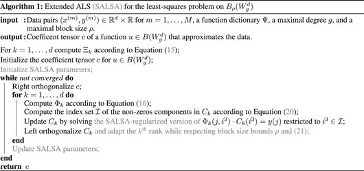
Algorithm 1. Extended ALS (SALSA) for the least-squares problem on
To optimize the coefficient tensors c(0), …, c(g) in the space
which can be solved using Algorithm 1. The original problem Eq. 14 is then solved by alternating over
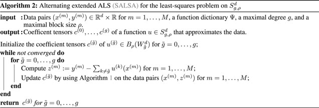
Algorithm 2. Alternating extended ALS (SALSA) for the least-squares problem on
The proposed representation has several advantages. The optimization with the tensor train structure is computationally less demanding than solving directly in
Remark 4.2. Let us comment on the practical pondering behind choosing
5 Numerical Results
In this section we illustrate the numerical viability of the proposed framework on some simple but common problems. We estimate the relative errors on test sets with respect to the sought function f and are interested in the required number of samples leading to recovery. Our implementation is meant only as a proof of concept and does not lay any emphasis on efficiency. The rank is chosen a priori, the stopping criteria are naïvely implemented and rank adaptivity, as would be provided by SALSA, is missing all together.3 For this reason we only compare the methods in terms of degrees of freedom and accuracy and not in terms of computing time. These are relevant quantities nonetheless, since the degrees of freedom are often the limiting factor in high dimensions and the computing time is directly related to the number of degrees of freedom.
In the following we always assume p = g + 1. We also restrict the group sizes to be bounded by the parameter ρmax. In our experiments we choose ρmax without any particular strategy but ideally, ρmax would be determined adaptively by the use of SALSA, which we did not do in this work. For every sample size the error plots show the distribution of the errors between the 0.15 and 0.85 quantile. The code for all experiments has been made publicly available at https://github.com/ptrunschke/block_sparse_tt.
5.1 Riccati Equation
In this section we consider the closed-loop linear quadratic optimal control problem
After a spatial discretization of the heat equation with finite differences we obtain a d-dimensional system of the form
It is well known [47] that the value function for this problem takes the form
In this experiment we use the dictionary of monomials Ψ = Ψmonomial (cf. Eq. 4) and compare the ansatz spaces
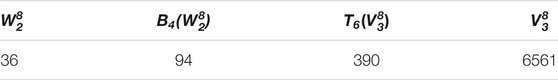
TABLE 1. Degrees of freedom for the full space
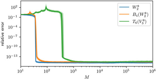
FIGURE 1. 0.15–0.85 quantiles for the recovery error in
A clever change of basis, given by the diagonalization of Q, can reduce the required block size from 4 to 1. This allows to extend the presented approach to higher dimensional problems. The advantage over the classical Riccati approach becomes clear when considering non-linear versions of the control problem that do not exhibit a Riccati solution. This is done in [8,9] using the dense TT-format
5.2 Gaussian Density
As a second example we consider the reconstruction of an unnormalized Gaussian density
again on the domain Ω = [−1,1]d with d = 6. For the dictionary Ψ = ΨLegendre [cf. Eq. 5] we chose g = 7, ρmax = 1 and r = 8 and compare the reconstruction w.r.t.
and can therefore be well approximated as a rank 1 tensor train with each component Ck just being a best approximation for
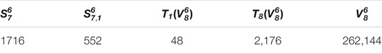
TABLE 2. Degrees of freedom for the full space
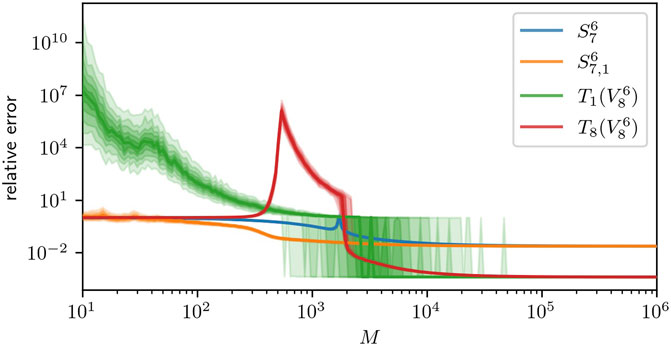
FIGURE 2. 0.15–0.85 quantiles for the recovery error in
5.3 Quantities of Interest
The next considered problem often arises when computing quantities of interest from random partial differential equations. We consider the stationary diffusion equation
on D = [−1,1]2. This equation is parametric in y ∈ [−1,1]d. The randomness is introduced by the uniformly distributed random variable
with
An important result proven in [31] ensures the ℓp summability, for some 0 < p ≤ 1, of the polynomial coefficients of the solution of this equation in the dictionary of Chebyshev polynomials. This means that the function is very regular and we presume that it can be well approximated in
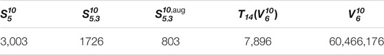
TABLE 3. Degrees of freedom for the full space
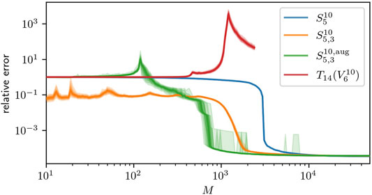
FIGURE 3. 0.15–0.85 quantiles for the recovery error in
6 Conclusion
We introduce block sparsity [28,29] as an efficient tool to parametrize, multivariate polynomials of bounded degree. We discuss how to extend this to general multivariate polynomials of bounded degree and prove bounds for the block sizes for certain polynomials. As an application we discuss the problem of function identification from data for tensor train based ansatz spaces and give some insights into when these ansatz spaces can be used efficiently. For this we motivate the usage of low degree multivariate polynomials by approximation results (e.g. [30,31]) and recent results on sample complexity [32]. This leads to a novel algorithm for the problem at hand. We then demonstrate the applicability of this algorithm to different problems. Up until now block sparse tensor trains are not used for these recovery tasks. The numerical examples, however, demonstrate that at least dense tensor trains can not compete with our novel block-sparse approach. We observe that the sample complexity can be much more favorable for successful system identification with block sparse tensor trains than with dense tensor trains or purely sparse representations. We expect that the inclusion of rank-adaptivity using techniques from SALSA or bASD is straight forward, which we therefore consider an interesting direction from an applied point of view for forthcoming papers. We expect, that this would improve the numerical results even further. The introduction of rank-adaptivity would moreover alleviate the problem of having to choose a block size a-priori. Finally, we want to reiterate that the spaces of polynomials with bounded degree are predestined for the application of least-squares recovery with an optimal sampling density (cf [39]) which holds opportunities for further improvement of the sample efficiency. This leads us to the strong believe that the proposed algorithm can be applied successfully to other high dimensional problems in which the sought function exhibits sufficient regularity.
Data Availability Statement
The datasets presented in this study can be found in online repositories. The names of the repository/repositories and accession number(s) can be found below: https://github.com/ptrunschke/block_sparse_tt.
Author Contributions
MG is the main contributor of the block-sparse tensor train section. RS is the main contributor of the method section. PT is the main contributor of the sample complexity section, the implementation of the experiments and contributed to the proof of the main Theorem. All authors contributed to every section and contributed equally to the introduction and to the discussion.
Funding
MG was funded by DFG (SCHN530/15-1). RS was supported by the Einstein Foundation Berlin. PT acknowledges support by the Berlin International Graduate School in Model and Simulation based Research (BIMoS).
Conflict of Interest
The authors declare that the research was conducted in the absence of any commercial or financial relationships that could be construed as a potential conflict of interest.
Publisher’s Note
All claims expressed in this article are solely those of the authors and do not necessarily represent those of their affiliated organizations, or those of the publisher, the editors and the reviewers. Any product that may be evaluated in this article, or claim that may be made by its manufacturer, is not guaranteed or endorsed by the publisher.
Footnotes
1It is possible to include rank adaptivity as in SALSA [21] or bASD [13] and we have noted this in the relevant places.
2The orthogonality comes from the symmetry of L which results in orthogonal eigenspaces.
3We expect, that an application of the state-of-the-art SALSA algorithm to the block-sparse model class, as described in Section 4, is straight forward.
References
1. Brunton, SL, Proctor, JL, and Kutz, JN. Discovering Governing Equations from Data by Sparse Identification of Nonlinear Dynamical Systems. Proc Natl Acad Sci USA (2016) 113(15):3932–7. doi:10.1073/pnas.1517384113
2., Gelß, P, Klus, S, Eisert, J, and Schütte, C. Multidimensional Approximation of Nonlinear Dynamical Systems. J Comput Nonlinear Dyn (2019) 14(6). doi:10.1115/1.4043148
3. Goeßmann, A, Götte, M, Roth, I, Ryan, S, Kutyniok, G, and Eisert, J. Tensor Network Approaches for Data-Driven Identification of Non-linear Dynamical Laws (2020). NeurIPS2020 - Tensorworkshop.
4. Kazeev, V, and Khoromskij, BN. Low-Rank Explicit QTT Representation of the Laplace Operator and its Inverse. SIAM J Matrix Anal Appl (2012) 33(3):742–58. doi:10.1137/100820479
5. Kazeev, V, and Schwab, C. Quantized Tensor-Structured Finite Elements for Second-Order Elliptic PDEs in Two Dimensions. Numer Math (2018) 138(1):133–90. doi:10.1007/s00211-017-0899-1
6. Bachmayr, M, and Kazeev, V. Stability of Low-Rank Tensor Representations and Structured Multilevel Preconditioning for Elliptic PDEs. Found Comput Math (2020) 20(5):1175–236. doi:10.1007/s10208-020-09446-z
7. Eigel, M, Pfeffer, M, and Schneider, R. Adaptive Stochastic Galerkin FEM with Hierarchical Tensor Representations. Numer Math (2016) 136(3):765–803. doi:10.1007/s00211-016-0850-x
8. Dolgov, S, Kalise, D, and Kunisch, K. Tensor Decomposition Methods for High-Dimensional Hamilton-Jacobi-Bellman Equations. arXiv (2021). 1908.01533 [cs, math].
9. Oster, M, Sallandt, L, and Schneider, R. Approximating the Stationary Hamilton-Jacobi-Bellman Equation by Hierarchical Tensor Products. arXiv (2021). arXiv:1911.00279 [math].
10. Richter, L, Sallandt, L, and Nüsken, N. Solving High-Dimensional Parabolic PDEs Using the Tensor Train Format. arXiv (2021). arXiv:2102.11830 [cs, math, stat].
11. Christian, B, Martin, E, Leon, S, and Philipp, T. Pricing High-Dimensional Bermudan Options with Hierarchical Tensor Formats. arXiv (2021). arXiv:2103.01934 [cs, math, q-fin].
12. Glau, K, Kressner, D, and Statti, F. Low-Rank Tensor Approximation for Chebyshev Interpolation in Parametric Option Pricing. SIAM J Finan Math (2020) 11(3):897–927. Publisher: Society for Industrial and Applied Mathematics doi:10.1137/19m1244172
13. Eigel, M, Neumann, J, Schneider, R, and Wolf, S. Non-intrusive Tensor Reconstruction for High-Dimensional Random PDEs. Comput Methods Appl Math (2019) 19(1):39–53. doi:10.1515/cmam-2018-0028
14. Eigel, M, Schneider, R, Trunschke, P, and Wolf, S. Variational Monte Carlo–Bridging Concepts of Machine Learning and High-Dimensional Partial Differential Equations. Adv Comput Math (2019) 45(5):2503–32. doi:10.1007/s10444-019-09723-8
15. Zhang, Z, Yang, X, Oseledets, IV, Karniadakis, GE, and Daniel, L. Enabling High-Dimensional Hierarchical Uncertainty Quantification by Anova and Tensor-Train Decomposition. IEEE Trans Comput.-Aided Des Integr Circuits Syst (2015) 34(1):63–76. doi:10.1109/tcad.2014.2369505
16. Klus, S, and Gelß, P. Tensor-Based Algorithms for Image Classification. Algorithms (2019) 12(11):240. doi:10.3390/a12110240
17. Stoudenmire, E, and Schwab, DJ “Advances in Neural Information Processing Systems,” in Supervised Learning with Tensor Networks. Editors D. Lee, M. Sugiyama, U. Luxburg, I. Guyon, and R. Garnett. Curran Associates, Inc. (2016) 29. Available at: https://proceedings.neurips.cc/paper/2016/file/5314b9674c86e3f9d1ba25ef9bb32895-Paper.pdf/
18. Oseledets, IV. DMRG Approach to Fast Linear Algebra in the TT-Format. Comput Methods Appl Math (2011) 11(3):382–393. doi:10.2478/cmam-2011-0021
19. Holtz, S, Rohwedder, T, and Schneider, R. The Alternating Linear Scheme for Tensor Optimization in the Tensor Train Format. SIAM J Sci Comput (2012) 34(2):A683–A713. doi:10.1137/100818893
20. White, SR. Density Matrix Formulation for Quantum Renormalization Groups. Phys Rev Lett (1992) 69(19):2863–6. doi:10.1103/physrevlett.69.2863
21. Grasedyck, L, and Krämer, S. Stable ALS Approximation in the TT-Format for Rank-Adaptive Tensor Completion. Numer Math (2019) 143(4):855–904. doi:10.1007/s00211-019-01072-4
22. Holtz, S, Rohwedder, T, and Schneider, R. On Manifolds of Tensors of Fixed TT-Rank. Numer Math (2012) 120(4):701–31. doi:10.1007/s00211-011-0419-7
23. Lubich, C, Oseledets, IV, and Vandereycken, B. Time Integration of Tensor Trains. SIAM J Numer Anal (2015) 53(2):917–41. doi:10.1137/140976546
24. Chevreuil, M, Lebrun, R, Nouy, A, and Rai, P. A Least-Squares Method for Sparse Low Rank Approximation of Multivariate Functions. Siam/asa J Uncertainty Quantification (2015) 3(1):897–921. doi:10.1137/13091899x
25. Grelier, E, Anthony, N, and Chevreuil, M. Learning with Tree-Based Tensor Formats. arXiv (2019). arXiv:1811.04455 [cs, math, stat].
26. Grelier, E, Anthony, N, and Lebrun, R. Learning High-Dimensional Probability Distributions Using Tree Tensor Networks. arXiv (2021). arXiv:1912.07913 [cs, math, stat].
27. Haberstich, C. Adaptive Approximation of High-Dimensional Functions with Tree Tensor Networks for Uncertainty Quantification (2020) Theses, École centrale de Nantes.
28. Singh, S, Pfeifer, RNC, and Vidal., G. Tensor Network Decompositions in the Presence of a Global Symmetry. Phys Rev A (2010) 82(5):050301. doi:10.1103/physreva.82.050301
29. Markus, B, Michael, G, and Max, P. Particle Number Conservation and Block Structures in Matrix Product States. arXiv (2021). arXiv:2104.13483 [math.NA, quant-ph].
30. Breiten, T, Kunisch, K, and Pfeiffer, L. Taylor Expansions of the Value Function Associated with a Bilinear Optimal Control Problem. Ann de l'Institut Henri Poincaré C, Analyse non linéaire (2019) 36(5):1361–99. doi:10.1016/j.anihpc.2019.01.001
31. Hansen, M, and Schwab, C. Analytic Regularity and Nonlinear Approximation of a Class of Parametric Semilinear Elliptic PDEs. Mathematische Nachrichten (2012) 286(8-9):832–60. doi:10.1002/mana.201100131
32. Eigel, M, Schneider, R, and Trunschke, P. Convergence Bounds for Empirical Nonlinear Least-Squares. arXiv. arXiv:2001.00639 [cs, math], 2020.
35. Espig, M, Hackbusch, W, Handschuh, S, and Schneider, R. Optimization Problems in Contracted Tensor Networks. Comput Vis Sci. (2011) 14(6):271–85. doi:10.1007/s00791-012-0183-y
36. Oseledets, IVV. Tensor-Train Decomposition. SIAM J Sci Comput (2011) 33(5):2295–317. doi:10.1137/090752286
37. Hackbusch, W. On the Representation of Symmetric and Antisymmetric Tensors. Preprint. Leipzig, Germany: Max Planck Institute for Mathematics in the Sciences (2016).
38. Wolf, S. Low Rank Tensor Decompositions for High Dimensional Data Approximation, Recovery and Prediction. [PhD thesis]. TU Berlin (2019).
39. Cohen, A, and Migliorati, G. Optimal Weighted Least-Squares Methods. SMAI J Comput Math (2017) 3:181–203. doi:10.5802/smai-jcm.24
40. Haberstich, C, Anthony, N, and Perrin, G. Boosted Optimal Weighted Least-Squares. arXiv (2020). arXiv:1912.07075 [math.NA].
41. Göttlich, S, and Schillinger, T. Microscopic and Macroscopic Traffic Flow Models Including Random Accidents (2021).
42. Rasmussen, CE, and Williams, CKI. Gaussian Processes for Machine Learning. Cambridge: MIT Press (2006).
43. Cornford, D, Nabney, IT, and Williams, CKI. Modelling Frontal Discontinuities in Wind fields. J Nonparametric Stat (2002) 14(1-2):43–58. doi:10.1080/10485250211392
44. Szalay, S, Pfeffer, M, Murg, V, Barcza, G, Verstraete, F, Schneider, R, et al. Tensor Product Methods and Entanglement Optimization Forab Initioquantum Chemistry. Int J Quan Chem. (2015) 115(19):1342–91. doi:10.1002/qua.24898
45. Michel, B, and Nouy, A. Learning with Tree Tensor Networks: Complexity Estimates and Model Selection. arXiv (2021). arXiv:2007.01165 [math.ST].
46. Ballani, J, and Grasedyck, L. Tree Adaptive Approximation in the Hierarchical Tensor Format. SIAM J Sci Comput (2014) 36(4):A1415–A1431. doi:10.1137/130926328
47. Curtain, RF, and Hans, Z. An Introduction to Infinite-Dimensional Linear Systems Theory. New York: Springer (1995).
Keywords: sample efficiency, homogeneous polynomials, sparse tensor networks, alternating least square, empirical L2 approximation
Citation: Götte M, Schneider R and Trunschke P (2021) A Block-Sparse Tensor Train Format for Sample-Efficient High-Dimensional Polynomial Regression. Front. Appl. Math. Stat. 7:702486. doi: 10.3389/fams.2021.702486
Received: 29 April 2021; Accepted: 21 July 2021;
Published: 07 September 2021.
Edited by:
Edoardo Angelo Di Napoli, Helmholtz-Verband Deutscher Forschungszentren (HZ), GermanyReviewed by:
Mazen Ali, École centrale de Nantes, FranceKatharina Kormann, Uppsala University, Sweden
Antonio Falco, Universidad CEU Cardenal Herrera, Spain
Copyright © 2021 Götte, Schneider and Trunschke. This is an open-access article distributed under the terms of the Creative Commons Attribution License (CC BY). The use, distribution or reproduction in other forums is permitted, provided the original author(s) and the copyright owner(s) are credited and that the original publication in this journal is cited, in accordance with accepted academic practice. No use, distribution or reproduction is permitted which does not comply with these terms.
*Correspondence: Philipp Trunschke, cHRydW5zY2hrZUBtYWlsLnR1LWJlcmxpbi5kZQ==