 Ronan Fablet
 Maxime Beauchamp1
 Lucas Drumetz
- 1IMT Atlantique, UMR CNRS Lab-STICC, Brest, France
- 2IMT Atlantique, UMR INSERM LaTIM, Brest, France
Earth observation satellite missions provide invaluable global observations of geophysical processes in play in the atmosphere and the oceans. Due to sensor technologies (e.g., infrared satellite sensors), atmospheric conditions (e.g., clouds and heavy rains), and satellite orbits (e.g., polar-orbiting satellites), satellite-derived observations often involve irregular space–time sampling patterns and large missing data rates. Given the current development of learning-based schemes for earth observation, the question naturally arises whether one might learn some representation of the underlying processes as well as solve interpolation issues directly from these observation datasets. In this article, we address these issues and introduce an end-to-end neural network learning scheme, which relies on an energy-based formulation of the interpolation problem. This scheme investigates different learning-based priors for the underlying geophysical field of interest. The end-to-end learning procedure jointly solves the reconstruction of gap-free fields and the training of the considered priors. Through different case studies, including observing system simulation experiments for sea surface geophysical fields, we demonstrate the relevance of the proposed framework compared with optimal interpolation and other state-of-the-art data-driven schemes. These experiments also support the relevance of energy-based representations learned to characterize the underlying processes.
1 Introduction
When dealing with spaceborne earth observation, available observation datasets do not involve gap-free and regularly gridded signals or images. The irregular sampling may result both from the characteristics of the sensors and sampling strategy, for example, considered orbits and swaths, as well as environmental conditions which may affect the sensor, for example, atmospheric conditions and clouds for earth observation. This is a critical feature to be dealt with to fully exploit the potential of available satellite-derived earth observation dataset.
A rich literature exists on interpolation for irregularly sampled signals and images (also referred to as inpainting in image processing (Bertalmio et al., 2000)). A classic framework states the interpolation issue as the minimization of an energy, which may be interpreted in a Bayesian framework. A variety of energy forms have been considered, including Markovian priors (Freeman and Liu, 2011), patch-based priors (Peyr et al., 2011), gradient norms in variational and/or PDE-based formulations (Bertalmio et al., 2000), and Gaussian priors (Galerne et al., 2011), as well as dynamical priors in fluid dynamics (Bertalmio et al., 2001). It also relates to optimal interpolation and kriging (Cressie and Wikle, 2015), which are among the state-of-the-art operational schemes in geoscience (Evensen, 2009). Optimal interpolation schemes classically involve the inference of the considered covariance-based priors from irregularly sampled data. This may however be at the expense of Gaussianity and linearity assumptions, which do not often apply for real signals and images. For the other types of energy forms, their parameterizations are generally set a priori and not learned from the data. Regarding more particularly data-driven and learning-based approaches, most previous works (Peyr et al., 2011; Alvera-Azcarate et al., 2016; Fablet et al., 2017) have addressed the learning of interpolation schemes under the assumption that a representative gap-free dataset is available. This gap-free dataset may be the image itself (Criminisi et al., 2004; Lorenzi et al., 2011; Peyr et al., 2011). For numerous application domains, as mentioned above, this assumption cannot be fulfilled. Regarding recent advances in learning-based schemes, a variety of deep learning models (e.g., Chen et al., 2015; Liu et al., 2018; Xie et al., 2012) have been proposed. Most of these works focus on learning an interpolator. One may however expect to learn not only an interpolator but also some representation of the considered data, which may be of interest for other applications. In this respect, RBM models (restricted Boltzmann machines) (Salakhutdinov and Hinton, 2009; Chen et al., 2015) are particularly appealing at the expense, however, of computationally expensive MCMC (Markov chain Monte Carlo) schemes.
In this article, we aimed to jointly learn representations of 2 days or 2 days + t processes from irregularly sampled observation datasets and solve the associated interpolation issue. Our contribution is three-fold:
• An end-to-end learning of energy-based representations from irregularly sampled training data. Based on a neural network architecture backed by a variational formulation, it jointly embeds the considered energy form and an associated interpolation scheme.
• Besides classic auto-encoder representations, we introduce neural network–based Gibbs energy representations, which relate to Gibbs priors embedded in convolutional neural networks (CNNs).
• The demonstration of the relevance of the proposed end-to-end learning framework, especially for very high missing data rates in spatiotemporal satellite-derived sea surface fields.
The remainder is organized as follows. Section 2 formally states the considered issue. We introduce the proposed end-to-end learning scheme in Section 3. We report numerical experiments in Section 4 and discuss our contribution with respect to related work in Section 5.
2 Problem Statement
In this section, we formally introduce the considered issue, namely, the end-to-end learning of representations and interpolators from irregularly sampled data. Within a classic Bayesian or an energy-based framework, interpolation issues may be stated as a minimization issue.
where X is the considered signal, image, or image series (referred to hereafter as the hidden state); Y the observation data, only available on a subdomain
We assume we are provided with a series of irregularly sampled observations, that is, to say a set
We expect interpolation
Assuming state X is a zero-mean multivariate random variable,
Here, we do not restrict to linear quadratic priors, and we aim to learn the parameters θ of energy
where
Given this general formulation, the end-to-end learning issue comes to solve minimization (Eq. 4) according to some given parameterization of energy
3 Proposed End-To-End Learning Framework
In this section, we detail the proposed neural network–based implementation of the end-to-end formulation introduced in the previous section. We first present the considered paramaterizations for energy
3.1 NN-Based Energy Formulation
We first investigate NN-based energy representations based on auto-encoders (LeCun et al., 2015). Let us denote the encoding and decoding operators of an auto-encoder (AE) by
Minimizing (Eq. 1) according to this energy amounts to retrieving state X whose low-dimensional representation in the encoding space matches the observed data in the original decoded space. Here, parameters θ comprise the parameters of the encoder
The mapping to a lower-dimensional space may be regarded as a likely loss in the representation potential. Gibbs models provide an appealing framework for an alternative energy-based representation, with no such dimensionality reduction constraint. Gibbs models introduced in statistical physics have also been widely explored in computer vision and pattern recognition (Geman, 1990) from the 80s. Gibbs models relate to the decomposition of
where
We implement this type of Gibbs energy using the following NN-based parameterization of operator ψ:
It involves the composition of a space and/or time convolutional operator
Overall, we may use the following common formulation for the two types of energy-based representations:
They differ in the parameterization chosen for operator ψ and in the associated assumption on some underlying lower-dimensional space or manifold which describes the considered state X.
3.2 NN-Based Interpolator
Besides the NN-based energy formulation, the general formulation stated in Eq. 4 involves the definition of interpolation operator
Given parameterization (Eq. 8), a simple fixed-point algorithm may be considered to solve for (Eq. 4). This algorithm is at the basis of DINEOF algorithm and matrix completion under subspace constraints (Alvera-Azcarate et al., 2016; Jain et al., 2013). Given some dictionary-based representation, including, for instance, principal component analysis (PCA), also referred to as empirical orthogonal function (EOF) in geoscience, and low-rank decomposition, these approaches iteratively apply projections onto the considered dictionary-based representation. Here, the projection of a given state X is given by
Interestingly, this algorithm is parameter free and can be readily implemented in an NN architecture, given the number of iterations to be considered. We may point out that a similar end-to-end architecture has also been proposed in Barth et al. (2020).
Given some initialization, one may also consider an iterative gradient-based descent which applies at each iteration k
where
and
Here,
Let us denote, respectively, by
3.3 End-To-End Architecture and Implementation Details
Given the parameterizations for energy
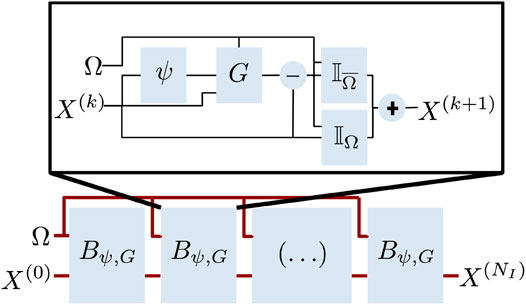
FIGURE 1. Sketch of the considered end-to-end architecture: We depict the considered
Regarding implementation details, beyond the design of the architectures, which may be application dependent for operators ψ and G (see Section 4), we consider an implementation under tensor flow/Keras. Regarding the training strategy, we use Adam optimizer. We iteratively increase the number of blocks
4 Experiments
In this section, we report numerical experiments on different datasets to evaluate and demonstrate the relevance of the proposed scheme. We first report numerical experiments on a simple synthetic 2D case study using MNIST data to gain insights on the different key components of the proposed framework. We then consider two observing system simulation experiments (OSSEs) corresponding to realistic sampling patterns for satellite-derived sea surface geophysical fields, namely, sea surface temperature (SST) derived from infrared satellite sensors and sea surface height (SSH) derived from narrow-swath and wide-swath satellite altimeters. In all experiments, we refer to the AE-based frameworks, respectively, as FP(d)-ConvAE and G(d)-ConvAE using the fixed-point or gradient-based interpolator, where d refers to the number of blocks
As evaluation metrics, we consider the reconstruction score computed over the observation domain, referred to as the R-score.
where
We also evaluate the quality of the trained representation ψ through the AE-score defined as
When considering the training scheme which only relies on observation data, that is, we never exploit the gap-free dataset during the training stage, we may compute these metrics both for the training and test datasets.
4.1 MNIST Case Study
We evaluate the proposed framework on MNIST dataset for which we simulate missing data patterns. MNIST dataset provides a dataset of 28 × 28 grayscale images of digits, which make it well suited for evaluation purposes. For this dataset, we only evaluate the AE-based setting. We consider the following convolutional AE architecture with a 20-dimensional encoding space:
• Encoder operator
• Decoder operator
This parameterization was selected from experiments on gap-free data to check that the resulting 20-dimensional representation accounts for more than 90% of the total variance of the MNIST test dataset. We noted experimentally that the training and interpolation performance did not vary a lot when modifying the parameteriration of the hidden layers of the encoder and decoder. In these experiments, we consider a batch size of 256. We used the reference training and test MNIST datasets. The training phase involved 100 epochs.
We generate random missing data patterns composed of
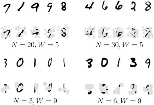
FIGURE 2. Illustration of the considered MNIST dataset with the selected missing data patterns: We randomly remove data from N
As mentioned above, we evaluate as performance measures an interpolation score (I-score), a global reconstruction score (R-score) for the interpolated images, and an auto-encoding (AE-score) score of the trained auto-encoder applied to gap-free data, in terms of explained variance. We also evaluate a classification score (C-score), in terms of mean accuracy, using the 20-dimensional encoding space as feature space for classification with a 3-layer multilayer perceptron (MLP). The results are consistent across the different missing data configurations. We report the performance measures for the test dataset in Table 1 for
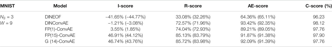
TABLE 1. Performance of AE schemes in the presence of missing data for the MNIST dataset: for a given convolutional AE architecture (see main text for details), the EOF and ConvAE models trained on gap-free data with a 15-iteration projection-based interpolation (resp., DINEOF and DINConvAE); a zero-filling strategy with the same ConvAE architecture, which can be regarded as an instance of the proposed scheme with a fixed-point solver using only one iteration (FP(1)-ConvAE); and the fixed-point and gradient-based versions of the proposed scheme. For each experiment, we evaluate four measures: the mean of the reconstruction performance for the known image areas (R-score), the interpolation performance for the missing data areas (I-score), the reconstruction performance of the trained AE when applied to gap-free images (AE score), and the classification score of a multilayer perceptron (MLP) classifier trained in the trained latent space for training images involving missing data. The metrics are evaluated for both the training dataset (first row of each model) and the test dataset (second row; numbers in parentheses). We report here the results for missing patterns with 3 9 × 9 missing data areas (
With a view to illustrating the training pattern of the considered end-to-end learning approach for the MNIST dataset, we display in Figure 3 the training loss and the I-score as a function of the number of epochs for a FP-ConvAE architecture and the missing data pattern given by
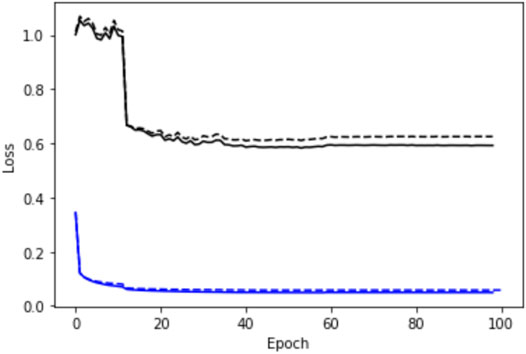
FIGURE 3. Illustration of the training pattern of the proposed end-to-end learning scheme: We plot the evolution of the training loss (blue) for the training (-) and the test (–) datasets as a function of the number of training epochs for a FP-ConvAE architecture and the MNIST dataset with three randomly sampled
For benchmarking purposes, we also report the performance of the DINEOF framework (Alvera-Azcarate et al., 2016; Ping et al., 2016), which uses a 20-dimensional EOF trained on the gap-free dataset; the auto-encoder architecture (ConvAE) also trained on a gap-free dataset, and the considered convolutional auto-encoder trained using an initial zero filling for missing data areas and a training loss computed only of observed data areas. The latter can be regarded as a FP(1)-ConvAE architecture using a single fixed-point block in Figure 1. Overall, for
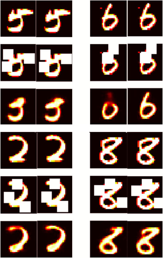
FIGURE 4. Illustration of reconstruction results for MNIST examples: For each panel, the first column refers to zero-ConvAE results and the second one to FP(15)-ConvAE. The first row depicts the reference image, the second row themissing datamask, and the third one the interpolated image. The first two panels illustrate interpolation results for training data and the last two for test data. We depict grayscale amid images using false colors to highlight differences.
In terms of representation power, the auto-encoder representations learned with missing data reach a representation score above 90%, which is only slightly below the score of the same architecture trained from gap-free data (AE scores of 91.0 vs. 92.3%). Similar conclusions can be drawn from the other missing data patterns as detailed in Supplementary Appendix: detailed results for the MNIST dataset. Overall, the proposed scheme guarantees a good representation in terms of AE score with an additional gain in terms of interpolation performance, typically between
4.2 Sea Surface Temperature (SST) Case Study
The second case study addresses satellite-derived sea surface temperature (SST) fields. Given their relatively high sampling in space and time, SST data play a key role in the analysis and reconstruction of upper ocean dynamics. Due to the sensitivity of high-resolution SST sensors to the cloud cover, SST datasets issued from infrared sensors may involve large missing data rates (typically, between 70 and 90%, see the second row of Figures 5, 6 for an illustration). For evaluation purposes, we consider an OSSE to build a groundtruthed dataset from high-resolution numerical simulations, namely, NATL60 data (Molines, 2018) and real cloud masks from the METOP AVHRR sensor (Ouala et al., 2018). We consider series of 128 × 512 images over eleven consecutive days from June to August at a 0.05 resolution in an open ocean region in the North East Atlantic from (40.58°N, 46.3°W) to (53.04°N, 16.18°W). Overall, we randomly sample 400 128 × 512 × 11 image series as training data and 150 as the test dataset.
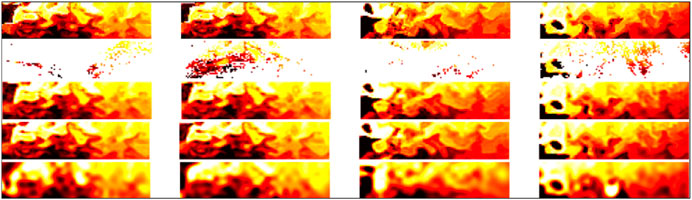
FIGURE 5. Interpolation examples for SST data used during training: the first row, reference SST images corresponding to the center of the considered 11-day time window; the second row, associated SST observations with missing data; the third row, interpolation issued from the FP(15)-GENN2 model; and the last row, reconstruction of the gap-free image series issued from the FP(15)-GENN2 model; interpolation issued from an OI scheme using a Gaussian covariance model with empirically tuned parameters.
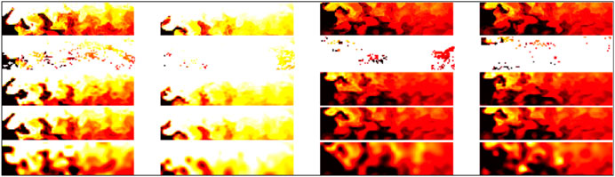
FIGURE 6. Interpolation examples for SST data never seen during training: the first row, reference SST images corresponding to the center of the considered 11 day time window; the second row, associated SST observations with missing data; the third row, interpolation issued from the FP(15)-GENN2 model; and the last row, reconstruction of the gap-free image series issued from the FP(15)-GENN2 model; interpolation issued from an OI scheme using a Gaussian covariance model with empirically tuned parameters.
For this case study, we consider the following four architectures for the AEs and the GENNs:
• ConvAE1: The first convolutional auto-encoder involves the following encoder architecture: five consecutive blocks with a Conv2D layer, a ReLu layer, and a 2 × 2 average pooling layer: the first one with 20 filters, the following four ones with 40 filters, and a final linear convolutional layer with 20 filters. The output of the encoder is 4 × 16 × 20. The decoder involves a Conv2DTranspose layer with ReLu activation for an initial 16 × 16 upsampling stage, a Conv2DTranspose layer with ReLu activation for an additional 2 × 2 upsampling stage, a Conv2D layer with 16 filters, and a last Conv2D layer with 5 filters. All Conv2D layers use 3 × 3 kernels. Overall, this model involves
• ConvAE2: We consider a more complex auto-encoder with an architecture similar to ConvAE1, where the number of filters is doubled (e.g., the output of the encoder is a 4 × 16 × 40 tensor). Overall, this model involves
• GENN1,2: We consider two GENN architectures. They share the same global architecture with an initial 4 × 4 average pooling, a Conv2D layer with ReLu activation with a zero-weight constraint on the center of the convolution window, a 1 × 1 Conv2D layer with N filters, a ResNet with a bilinear residual unit composed of an initial mapping to an initial 32 × 128x (5*N) space with a Conv2D + ReLu layer, a linear 1 × 1 Conv2D + ReLu layer with N filters, and a final 4 × 4 Conv2DTranspose layer with a linear activation for an upsampling to the input shape. GENN1 and GENN2 differ in the convolutional parameters of the first Conv2D layers and in the number of residual units. GENN1 involves 5 × 5 kernels,
These different parameterizations were selected so that ConvAE1 and GENN2 involve similar modeling complexities. Empirically, we noted that GENN architectures were more relevant when applied on a subsampled version of the SST fields. As such, the considered architecture for operator ψ involves an initial average pooling layer to subsample the spatial domain by a factor of four and a final upsampling block so that the output shape is the same size as the input shape. The application of GENNs to the finest resolution showed a lower performance. This is regarded as an illustration of the requirement for considering a scale-selection problem when applying a given prior. The upsampling block involves the combination of a Conv2DTranspose layer with 11 filters, a Conv2D layer with ReLu activation with 22 filters, and a linear Conv2D layer with 11 filters. Regarding the training procedure, we considered a batch size of 4, 400 epochs and an early stopping criterion to select the best performance on the training dataset. For benchmarking purposes, we proceed similar to the MNIST case study. As OI is the most widely applied interpolation method in geoscience, we include an OI with a Gaussian covariance model tuned using cross-validation.
Similar to the MNIST dataset, we report the performance of the different models in terms of interpolation score (I-score), reconstruction score (R-score), and the auto-encoding score (AE-score) both for the training and the test dataset. As for a given type of architecture for operator
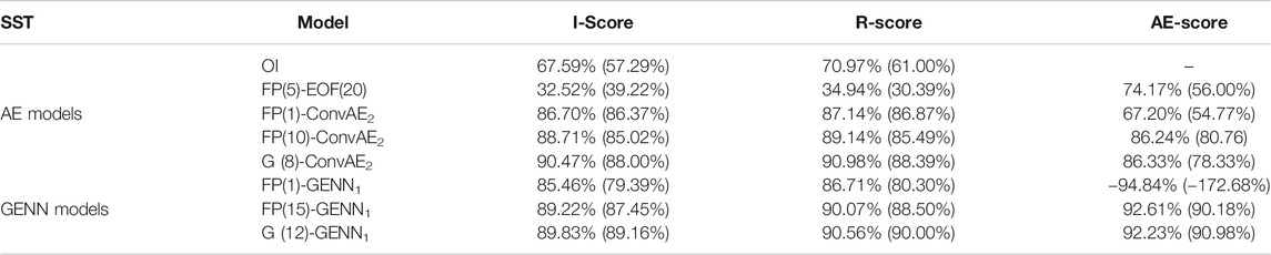
TABLE 2. Performance on the SST dataset: We evaluate for each model interpolation, reconstruction, and auto-encoding scores, respectively, I-score, R-score, and AE-score, in terms of percentage of explained variance, respectively, for the interpolation of missing data areas, the reconstruction of the whole fields with missing data, and the reconstruction of gap-free fields. For each model, we evaluate these scores for the training data (first row) and the test dataset (second row in brackets). In these experiments, we considered four different auto-encoder models: namely, 20- and 80-dimensional EOFs and ConvAE1,2 models and two GENN models. GENN1,2, combined with three interpolation strategies: the classic zero-filling strategy (zero), the proposed iterative fixed-point (FP) and gradient-based (G) schemes, the figure in brackets denoting the number of iterations. For instance, FP(10)-GENN1 refers to GENN1 with a 10-step fixed-point interpolation scheme. The EOFs are trained from gap-free data. We also consider an OI scheme with a space–time Gaussian covariance with empirically tuned parameters. We refer the reader to the main text for the detailed parameterization of the considered models. Here, we report, for each auto-encoder type, the best configuration in terms of the interpolation score. The detailed results are reported in Supplementary Appendix.
We illustrate these results in Figures 5, 6, which further stresses the gain with respect to OI for the reconstruction of finer-scale structures. The consistency between the interpolation results and the reconstruction of the gap-free image from the learned energy-based representation further stresses the ability of the proposed approach to extract a generic representation from irregularly sampled data. These results also emphasize a much greater ability of the proposed learning-based scheme to reconstruct finer structures, which can hardly be reconstructed by an OI scheme with a Gaussian space–time covariance model. We may recall that the latter is the state-of-the-art approach for the processing of satellite-derived earth observation data (Cressie and Wikle, 2015).
4.3 Sea Surface Height Case Study
This case study addresses satellite altimetry, which is the main source of observation data to retrieve sea surface currents on a global scale (Chelton and Wentz, 2005; Dufau et al., 2016). Current and upcoming satellite altimetry missions involve narrow-swath and wide-swath sensors on polar-orbiting satellites characterized by very high missing data rates with respect to a reference global grid, typically above 95% as illustrated in Figure 7. The space–time interpolation of satellite altimetry data is then a key challenge to produce sea surface current fields (Pascual et al., 2007; Ballarota et al., 2019). Here, we implement an OSSE for both nadir along-track altimeter data and of wide-swath altimeter data from the upcoming SWOT mission (Gaultier et al., 2015). For the former, we simulate the 2013 4-altimeter configuration for nadir along-track altimeter data. The OSSE relies on NATL60 high-resolution deterministic ocean simulation of the North Atlantic (Molines, 2018). As the case study region, we focus on a region along the Gulf Stream [33°N, 43°N; −65°W, −55°W] mainly driven by energetic mesoscale dynamics.
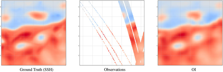
FIGURE 7. Illustration of the considered SSH dataset on April 8th, 2013: from left to right, reference SSH field (groundtruth), satellite-derived observation data (nadir along-track data and SWOT data), and optimally interpolated field (OI).
As baseline, we consider the operational processing chain for gridded altimeter fields, which relies on an OI scheme. All methods are applied to the anomaly with respect to this OI baseline. For benchmarking purposes, we run two state-of-the-art data-driven approaches, namely, the analog data assimilation (AnDA) (Lguensat et al., 2017) and the DINEOF algorithm (Ping et al., 2016). As for the SST case study, we train the EOF representation from the gap-free version of the training dataset. The AnDa scheme combines the exploitation of a gap-free reference dataset to design an analog dynamical model with a state-of-the-art ensemble Kalman filter to address the interpolation issue. Here, we implement the patch-based version of AnDA as presented in Fablet et al. (2017). As AnDA and DINEOF schemes rely on some training on a gap-free dataset, we use for evaluation purposes a 20-day test period in December, with the remaining data being used as training data except 10 days before and after the 20-day test period.
Regarding the proposed end-to-end learning framework, we consider architectures similar to the ones applied to the SST case study, namely, architectures ConvAE1 and GENN1 for operator ψ in (Eq. 5). To account for the knowledge of the OI baseline, states X and observations Y concatenate two components: a coarse-scale SSH component corresponding to the OI baseline and a fine-scale SSH component corresponding to the anomaly of the SSH field with respect to the OI baseline. Here, we consider 5-day time windows. This amounts to considering tensors X and Y of dimension 10 × 200 × 200. Similar to the SST case study, we gradually increased the number of iterations
Similar to the SST case study, we first applied the proposed unsupervised end-to-end learning strategy as synthesized in Table 3. As SSH fields involve a rather low contrast, we compute all performance metrics for the norm of the gradient of the SSH fields, which relate to the norm of sea surface current. We may notice that ConvAE architectures lead to poor performance and even degrade the reconstruction with respect to the OI baseline. These results suggest that auto-encoder architectures applied globally cannot account for the space–time variability observed in the case study area for spatial scales below a few hundreds of kilometers. This is particularly emphasized by poor AE scores. By contrast, GENN architectures seem more adapted with the best performance issued from the fixed-point solver. However, in the unsupervised case, we only report a relatively marginal gain with respect to the OI baseline. We hypothesize that this relates to the very high missing data rates. In such cases, we also noted an early stopping criterion to be necessary after 10 to 20 epochs to avoid over-fitting issues.
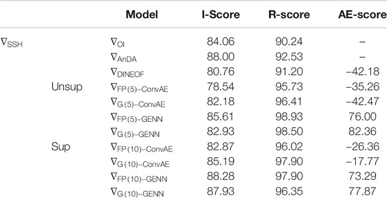
TABLE 3. Evalulation of the benchmarked methods for the SSH case study using an unsupervised and supervised training strategy: we evaluate for the gradient norm of the SSH fields
To further evaluate this point, we perform a supervised learning experiment, where all end-to-end learning architectures are trained to minimize the reconstruction of the true field, assuming we are provided with a fully groundtruthed gap-free training dataset. Interestingly, using such a supervised learning strategy, we report much greater improvement for the reconstruction of the SSH gradients, for example, I-scores of
In Figure 8, we visualize interpolation examples for specific data of the test period. They further illustrate the low relevance of DINEOF and ConvAE approaches to improve the reconstruction of SSH gradients with respect to the OI baseline. They also make clear the much better reconstruction performance of GENN architectures trained in a supervised fashion rather than in a non-supervised one. In these experiments, gradient-based end-to-end architectures may generate local artifacts, whereas the fixed-point ones appear more stable. We refer the reader to the study by Beauchamp et al. (2020) for a detailed intercomparison of data-driven approaches for the interpolation of SSH fields for different satellite altimeter datasets.
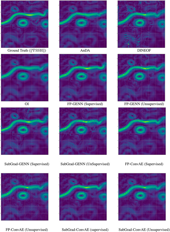
FIGURE 8. Comparison of data-driven interpolation methods for the norm of the gradient of the SSH field on April 8th, 2013: reference SSH field (groundtruth), optimally interpolated field (OI) (left panel), and data-driven interpolations of the SSH field using DINEOF, AnDA, FP(5)-ConvAE, and FP(5)-GENN methods. We refer the reader to the main text for details on these methods.
5 Related and Future Work
This section further discusses the proposed framework with respect to the related work, especially optimal interpolation, learning-based interpolator, and energy-based representation of signals and images.
Optimal interpolation: As stated in (Eq. 3), OI can be regarded as a relaxed version of (Eq. 1), where energy
Learning interpolators: A significant amount of work has been dedicated to the development of learning-based schemes for interpolation issues. Regarding deep learning models, most of the proposed approaches focus on directly learning the interpolation algorithms using some initialization, typically a zero-filling initialization (Xie et al., 2012; Yan et al., 2018). Examples of such approaches include both auto-encoder–like CNN architectures (Xie et al., 2012; Yan et al., 2018) and CNN architectures inspired from reaction–diffusion PDEs (Chen et al., 2015) derived from variational formulations (Bertalmio et al., 2000). Rather than deriving the architecture from the gradient descent algorithm associated with some a priori energy formulation, we here aimed to jointly learn an energy-based representation of the class of signals or images of interest and the NN-based implementation of the associated minimization scheme. Regarding the latter, we have shown that the parameter-free fixed-point architecture may prove efficient. In Barth et al. (2020), a similar end-to-end architecture is proposed; however, it does not explicitly rely on an underlying variational formulation and only explores auto-encoder architecture. Recent studies have also investigated the learning of variational formulations associated with gradient-based solvers (Kobler et al., 2020). Gradient-based solvers appear more flexible than fixed-point ones to account for more complex observation models. In this context, future work could further explore and benchmark the derivation and learning of computationally efficient minimization architectures including using ideas from meta-learning approaches (Hospedales et al., 2020).
Representation learning and energy-based representations: Representation learning is among the key feature of deep learning methods to infer relevant computational representations of some underlying processes given observation data (Bengio et al., 2013). One may cite a variety of case studies showing neural networks trained on a given task embedded in some representation, which is of interest for many other tasks. Here, we consider the auto-encoder score to evaluate the representation capacity of a model trained from irregularly sampled data. Our results point out that given some appropriate design of the end-to-end architecture, the model learned from data with very high missing data rates can infer a relevant representation of the gap-free states. To this end, we rely on energy-based representations. Such representations have been widely explored as such representations are the core of physics-informed representations, for example, Gibbs models in statistical physics and Hamiltonian representations in mechanics (Geman, 1990). From the mid-70s, both continuous and discrete energy representations have been considered in signal and image processing to address inverse problems. Among others, we may cite denoising, interpolation, segmentation, and super-resolution issues (Geman, 1990; Roth and Black, 2009; Freeman and Liu, 2011). In Roth and Black (2009), higher-order Markovian fields were investigated with nonlinear functions of many filter responses. Similar to these energy priors, the proposed GENN architecture decomposes as a sum of terms which only involves local neighborhoods. The latter relates to the Markovian property embedded in Gibbs priors. Whereas the calibration of such Gibbs models generally involves a relatively low number of parameters, their NN-based implementation allows us to consider much more complex parameterizations as well as to learn such representations in unobserved (latent) spaces. In the reported application, we consider an energy-based representation in a downscaled version of the considered spatial domain and learn the associated upscaling operator. As shown here, it also provides new means to jointly learn such priors and solve the associated inverse problem when considering irregularly sampled training data. Regarding deep learning models, restricted Boltzman machines (RBMs) are active research topics (Salakhutdinov and Hinton, 2009; Zhang et al., 2018). They also involve an energy-based formulation which relates the observed data to latent variables. A number of applications support their relevance, including when dealing with missing data. Numerically speaking, they exploit MCMC techniques, which are computationally expensive and may make their combination with other DL architectures more difficult. Here, through the considered parameterization (Eq. 8), we can derive simple and efficient inversion schemes from a learned energy representation. This property may open new avenues for a plug-and-play exploitation of such trainable priors for addressing other tasks than those considered during training. Besides, future work may also extend the proposed framework to trainable observation models.
Dealing with missing data: As stated in the introduction, dealing with missing data is often critical to address real-world issues and datasets, especially in spaceborne earth observation. Missing data may be due to sensor characteristics (sensitivity to acquisition conditions, acquisition sampling patterns, …) as well as to intrinsic features of the considered systems and processes. As a typical example, ocean dynamics (e.g., currents and geophysical tracer dynamics) are only defined within the ocean. Hence, the application of deep learning schemes to gridded representations of the ocean has to deal with missing data areas, including land areas. Given the texture-like and relatively low-contrast patterns depicted by geophysical dynamics, zero-filling strategies are most likely to lead to artifacts. CNNs defined on irregular graphs (Defferrard et al., 2016; Vialatte et al., 2016) may be an alternative. Here, we consider another alternative where the trainable energy-based representation applies to the entire regularly gridded domain. Among others, the proposed approach makes, for instance, the learning of representations feasible, which apply both on the open ocean (in areas with no land regions) and in coastal areas. Overall, future work will further explore the potential of the proposed framework for the identification and exploitation of deep learning representations for the characterization, modeling, and reconstruction of geophysical dynamics from satellite remote sensing data.
Unsupervised vs. supervised learning: The reported experiments suggest that for missing rates up to 80% of the considered domain, as illustrated by MNIST and SST case studies, we may be able to learn directly the interpolation scheme and the underlying variational representation from observation datasets involving gaps. This is of key interest for a plug-and-play application to real datasets with no preprocessing steps. We also expect the proposed AE and GENN architectures to be flexible and generic to adapt to a variety of multivariate signals, images, and image time series. For larger missing data above 90%, the experiments reported for the SSH case study suggest that the training phase should be constrained by complementary data to lead to a relevant interpolation performance. Whereas we tested an idealized fully supervised setting, one may expect the same performance with a reference target dataset with gaps if the latter is sufficiently large. For a given observing system, such a reference dataset could be provided by another observing system, which could sense the considered process for specific time periods and/or regions, possibly according to an irregular space–time sampling. These results open research avenues to further investigate irregularly sampled multisensor datasets during the training phase of the proposed end-to-end architecture. The fast-sampling phase of the upcoming SWOT mission could be a typical example (Gaultier et al., 2015). During this fast-sampling phase, some ocean regions will involve a better space–time sampling. As such, one could explore the related SSH datasets as relevant groundtruthed reference datasets to train end-to-end architectures using as inputs other narrow-swath altimeters as well as other sea surface tracers. Here, we believe that multimodal extensions of the proposed framework could be of key interest.
Data Availability Statement
The data used in the reported experiments are available from the following link: https://github.com/CIA-Oceanix/DINAE_keras.
Author Contributions
RF, LD, and FR have designed the proposed methodology. RF and MB. have implemented the proposed framework and run numerical experiments. RF and MB have prepared the original draft.
Funding
This work was supported by LEFE program (LEFE MANU project IA-OAC), CNES (grant SWOT-DIEGO), and ANR Projects Melody and OceaniX. It benefited from HPC and GPU resources from Azure (Microsoft EU Ocean awards) and from GENCI-IDRIS (Grant 2020-101030).
Conflict of Interest
The authors declare that the research was conducted in the absence of any commercial or financial relationships that could be construed as a potential conflict of interest.
Supplementary Material
The Supplementary Material for this article can be found online at: https://www.frontiersin.org/articles/10.3389/fams.2021.655224/full#supplementary-material
References
Alvera-Azcárate, A., Barth, A., Parard, G., and Beckers, J.-M. (2016). Analysis of SMOS sea surface salinity data using DINEOF. Remote Sensing Environ. 180, 137–145. doi:10.1016/j.rse.2016.02.044
Ballarotta, M., Ubelmann, C., Pujol, M.-I., Taburet, G., Fournier, F., Legeais, J.-F, et al. (2019). On the resolutions of ocean altimetry maps. Ocean Sci. 15, 1091–1109. doi:10.5194/os-15-1091-2019
Barth, A., Alvera-Azcárate, A., Licer, M., and Beckers, J.-M. (2020). DINCAE 1.0: a convolutional neural network with error estimates to reconstruct sea surface temperature satellite observations. Geosci Model Dev. 13, 1609–1622. doi:10.5194/gmd-13-1609-2020
Beauchamp, M., Fablet, R., Ubelmann, C., Ballarotta, M., and Chapron, B. (2020). Intercomparison of Data-Driven and Learning-Based Interpolations of Along-Track Nadir and Wide-Swath SWOT Altimetry Observations. Remote Sensing. 12(22), 3806. doi:10.3390/rs12223806
Bengio, Y., Courville, A., and Vincent, P. (2013). Representation Learning: A Review and New Perspectives. IEEE Trans Pattern Anal Mach Intell. 35, 1798–1828. doi:10.1109/tpami.2013.50
Bertalmio, M, Sapiro, G, Caselles, V, and Ballester, C (2000). Image inpainting. ACM SIGGRAPH, 417–424. doi:10.1145/344779.344972
Bertalmio, M, Bertozzi, AL, and Sapiro, G (2001). Navier-Stokes, fluid dynamics, and image and video inpainting. Proc IEEE CVPR. 355–362.
Boyd, S., Parikh, N, Chu, E, Peleato, B, and Eckstein, J (2010). Distributed Optimization and Statistical Learning via the Alternating Direction Method of Multipliers. FNT Machine Learn. 3, 1–122. doi:10.1561/2200000016
Chelton, D. B., and Wentz, F. J. (2005). Global Microwave Satellite Observations of Sea Surface Temperature for Numerical Weather Prediction and Climate Research. Bull Amer Meteorol Soc. 86, 1097–1116. doi:10.1175/bams-86-8-1097
Chen, Y, Yu, W, and Pock, T (2015). On Learning Optimized Reaction Diffusion Processes for Effective Image Restoration. Proc IEEE CVPR 5261–5269.
Chen, C. L. P., Zhang, C.-Y., Chen, L., and Gan, M. (2015). Fuzzy Restricted Boltzmann Machine for the Enhancement of Deep Learning. IEEE Trans Fuzzy Syst 23, 2163–2173. doi:10.1109/tfuzz.2015.2406889
Cressie, N, and Wikle, C (2015). Statistics for Spatio-Temporal Data. Hoboken, NJ: John Wiley and Sons.
Criminisi, A., Perez, P., and Toyama, K. (2004). Region filling and object removal by exemplar-based image inpainting. IEEE Trans Image Process. 13, 1200–1212. doi:10.1109/tip.2004.833105
Defferrard, M, Bresson, X, and Vandergheynst, P (2016). Convolutional Neural Networks on Graphs with Fast Localized Spectral Filtering. Proc NIPS 3844–3852.
Dufau, C., Orsztynowicz, M., Dibarboure, G., Morrow, R., and Le Traon, P. Y. (2016). Mesoscale resolution capability of altimetry: Present and future. J Geophys Res Oceans. 121, 4910–4927. doi:10.1002/2015jc010904
Fablet, R., Viet, P. H., and Lguensat, R. (2017). Data-Driven Models for the Spatio-Temporal Interpolation of Satellite-Derived SST Fields. IEEE Trans Comput Imaging. 3:647–657. doi:10.1109/tci.2017.2749184
Freeman, WT, and Liu, C. (2011). Markov Random Fields for Super-Resolution. Advances in Markov Random Fields for Vision and Image Processing. Cambridge, MA: MIT Press.
Galerne, B., Gousseau, Y., and Morel, J.-M. (2011). Random Phase Textures: Theory and Synthesis. IEEE Trans Image Process 20(1), 257–267. doi:10.1109/tip.2010.2052822
Gaultier, L., Ubelmann, C., and Fu, L. L. (2015). The Challenge of Using Future SWOT Data for Oceanic Field Reconstruction. JAOT 33:119–126.
He, K, Zhang, X, Ren, S, and Sun, J (2016). Deep Residual Learning for Image Recognition IEEE CPVR, Las Vegas, USA (IEEE). doi:10.1109/cvpr.2016.90
Hospedales, T, Antoniou, A, Micaelli, P, and Storkey, A (2020). Meta-learning in Neural Networks: A Survey.arXiv:200405439.
Jain, P, Netrapalli, P, and Sanghavi, S (2013). Low-rank Matrix Completion Using Alternating Minimization. ACM STOC 665–674. doi:10.1145/2488608.2488693
Kobler, E, Effland, A, Kunisch, K, and Pock, T (2020). Total Deep Variation for Linear Inverse Problems. arXiv:200105005. doi:10.1109/CVPR.2015.7299163
LeCun, Y., Bengio, Y., and Hinton, G. (2015). Deep learning. Nature 521, 436–444. doi:10.1038/nature14539
Lguensat, R., Huynh Viet, P., Sun, M., Chen, G., Fenglin, T., Chapron, B., et al. (2017). Data-driven Interpolation of Sea Level Anomalies using Analog Data Assimilation. Remote Sens. 11(7), 858. doi:10.3390/rs11070858
Liu, G., Reda, F., Shih, K., Wang, T., Tao, A., and Catanzaro, B. (2018). Image Inpainting for Irregular Holes Using Partial Convolutions. Proc ECCV 85–100.
Lorenzi, L., Melgani, F., and Mercier, G. (2011). Inpainting Strategies for Reconstruction of Missing Data in VHR Images. IEEE Geosci Remote Sensing Lett 8, 914–918. doi:10.1109/lgrs.2011.2141112
Molines, J. M. (2018). MEOM configurations NATL60-CJM165: NATL60 code used for CJM165 experiment. Zenodo. doi:10.5281/zenodo.1210116
Ouala, S, Fablet, R., Herzet, C., Chapron, B., Pascual, A., Collard, F, et al. (2018). Neural-Network-based Kalman Filters for the Spatio-Temporal Interpolation of Satellite-derived Sea Surface Temperature. Rem Sens 20, 1791.
Pascual, A., Pujol, M.-I., Larnicol, G., Le Traon, P.-Y., and Rio, M.-H. (2007). Mesoscale mapping capabilities of multisatellite altimeter missions: First results with real data in the Mediterranean Sea. J Mar Syst. 65, 190–211. doi:10.1016/j.jmarsys.2004.12.004
Peyr, G, Bougleux, S, and Cohen, L (2011). Non-local Regularization of Inverse Problems. Inverse Probl Imaging 5, 511–530.
Ping, B, Su, F, and Meng, Y (2016). An Improved DINEOF Algorithm for Filling Missing Values in Spatio-Temporal Sea Surface Temperature Data. PLoS One 11, e0155928. doi:10.1371/journal.pone.0155928
Roth, S., and Black, M. J. (2009). Fields of Experts. Int J Comput Vis 82, 205–229. doi:10.1007/s11263-008-0197-6
Salakhutdinov, R, and Hinton, G (2009). Deep Boltzmann Machines. Artificial intelligence and statistics, Clearwater Beach, FL (PMLR). 448–455.
Vialatte, J, Gripon, V, and Mercier, G (2016). Generalizing the Convolution Operator to extend CNNs to Irregular Domains. arXiv: 1606.01166.
Xie, J, Xu, L, and Chen, E (2012). Image Denoising and Inpainting with Deep Neural Networks. Proc NIPS 341–349.
Yan, Z., Li, X., Li, M., Zuo, W., and Shan, S. (2018). Shift-Net: Image Inpainting via Deep Feature Rearrangement. Proc ECCV 11218, 3–19. doi:10.1007/978-3-030-01264-9_1
Yu, W, Heber, S, and Pock, T (2015). On Learning Optimized Reaction Diffusion Processes for Effective Image Restoration. Proc IEEE CVPR 5261–5269.
Keywords: earth observation, end-to-end learning, interpolation, representation learning, energy-based representation, deep learning
Citation: Fablet R, Beauchamp M, Drumetz L and Rousseau F (2021) Joint Interpolation and Representation Learning for Irregularly Sampled Satellite-Derived Geophysical Fields. Front. Appl. Math. Stat. 7:655224. doi: 10.3389/fams.2021.655224
Received: 18 January 2021; Accepted: 20 April 2021;
Published: 11 May 2021.
Edited by:
Xiaodong Luo, Norwegian Research Institute (NORCE), NorwayReviewed by:
Leonardo Azevedo, Universidade de Lisboa, PortugalKyungbook Lee, Kongju National University, South Korea
Copyright © 2021 Fablet, Beauchamp, Drumetz and Rousseau. This is an open-access article distributed under the terms of the Creative Commons Attribution License (CC BY). The use, distribution or reproduction in other forums is permitted, provided the original author(s) and the copyright owner(s) are credited and that the original publication in this journal is cited, in accordance with accepted academic practice. No use, distribution or reproduction is permitted which does not comply with these terms.
*Correspondence: Ronan Fablet, cm9uYW4uZmFibGV0QGltdC1hdGxhbnRpcXVlLmZy