Random-Walk, Agent-Level Pandemic Simulation (RAW-ALPS) for Analyzing Effects of Different Lockdown Measures

This article develops an agent-level stochastic simulation model, termed RAW-ALPS, for simulating the spread of an epidemic in a community. The mechanism of transmission is agent-to-agent contact, using parameters reported for the COVID-19 pandemic. When unconstrained, the agents follow independent random walks and catch infections due to physical proximity with infected agents. Under lockdown, an infected agent can only infect a coinhabitant, leading to a reduction in the spread. The main goal of the RAW-ALPS simulation is to help quantify the effects of preventive measures—timing and durations of lockdowns—on infections, fatalities, and recoveries. The model helps measure changes in infection rates and casualties due to the imposition and maintenance of restrictive measures. It considers three types of lockdowns: 1) whole population (except the essential workers), 2) only the infected agents, and 3) only the symptomatic agents. The results show that the most effective use of lockdown measures is when all infected agents, including both symptomatic and asymptomatic, are quarantined, while the uninfected agents are allowed to move freely. This result calls for regular and extensive testing of a population to isolate and restrict all infected agents.

1 Introduction

There is a great interest in stochastic modeling and analysis of medical, economical, and epidemiological data resulting from the ongoing COVID-19 pandemic [1]. Until a large amount of infection, treatment, vaccination, containment, and recovery data from this pandemic become available, the community will have to rely primarily on simulation models to help assess situations and to evaluate countermeasures [2]. Naturally, simulation systems that follow precise mathematical and statistical models will play an important role in understanding this dynamic and complex situation [3]. There have been a large number of models proposed in the past literature, relating to the spread of epidemics through human contact or otherwise. They can be broadly categorized in two main classes (a more detailed taxonomy of simulation models can be found in [4]):

1. Population-Level, Deterministic, Dynamic Models: A large number of epidemiological models have focused on coarse, population-level summaries, that is, counts of infected (I), susceptible (S), removed or recovered (R), etc., whose evolutions are governed by deterministic differential equations. The original model of this type is the Susceptible-Infected-Removed (SIR) model [5], proposed by Kermack and McKendrick in 1927, that uses ordinary differential equations to model a constrained growth of the counts in those three categories. Since then, researchers have developed several advancements and variations of this model, including the SIRD model [6] given by

$\begin{array}{l}\frac{dS}{dt}=-\frac{\beta I\left(t\right)S\left(t\right)}{N},\frac{dI}{dt}=\frac{\beta I\left(t\right)S\left(t\right)}{N}-\gamma I\left(t\right)-\mu D\left(t\right),\\ \frac{dR}{dt}=\gamma I\left(t\right),\frac{dD}{dt}=\mu I\left(t\right) .\end{array}(1)$

 The scalar parameters β, γ, and µ together control the dynamics of infections, recovery, and mortality. The zero-sum condition $dS\mathrm{/}dt\mathrm{+}dI\mathrm{/}dt\mathrm{+}dR\mathrm{/}dt\mathrm{+}dD\mathrm{/}dt\mathrm{=}0$ ensures constancy of the community size: $S\mathrm{(}t\mathrm{)+}I\mathrm{(}t\mathrm{)+}R\mathrm{(}t\mathrm{)+}D\mathrm{(}t\mathrm{)}=N$. Several studies have applied these general models to different epidemics, such as Ebola and SARS [7]. A recent article [8] extends this model to include hospitalizations and different strata of infections, and estimates these quantities from the Wuhan COVID-19 pandemic.

While they provide useful population-level summaries, these models do not generally focus on capturing spatial dynamics. Specifically, they do not explicitly model agent dynamics as residents move around in a community or across communities. Also, these models often provide deterministic outcomes, with no mechanism to incorporate randomness in the model. Several recent simulation models, focusing directly on the COVID-19 illness, also rely on such coarser community-level models [9].

2. Agent-Level Modeling: While dynamical evolutions of population variables are simple and effective, especially for the overall assessment, they do not take into account any social dynamics, human behavior, societal restrictions, and complexities of human interactions explicitly. The models that study these human-level factors and variables, while tracking disease at an individual level, are called agent-level models [10]. Here one models the mobility, health status, and interactions of individual subjects (agents) to construct an overall population-level picture in a bottom-up way. The advantages of agent-based models are that they are more detailed and one can vary the parameters of lockdown measures, such as social distancing, at a granular level to infer overall outcomes. Furthermore, these models have built-in stochastic components for agent motions, interactions, infections, and recoveries, thus enabling a more realistic simulation environment. Agent-based models have been discussed in several articles, including [4, 11–13] and so on. The importance of simulation-based analysis of epidemic spread is emphasized in Ref. [14] but with a focus on infection models within a host. Ref. [12] constructed a detailed agent-based model for spread of infectious diseases, taking into account population demographics and other social conditions, but they did not consider countermeasures such as lockdowns in their simulations. A broad organization of different agent-based simulation methods has been presented in Ref. [4]. A recent article [15] studies the socioeconomic impact of social distancing using agent-based models. Although there are numerous other articles on the topic of agent-based simulations for simulating the spread of infections, we have only listed the most relevant ones.

In this article, we develop a mathematical simulation model, named RAW-ALPS, to simulate the spread of an infectious disease, such as COVID-19, in a confined community and to study the influence of some external interventions on outcomes. Since RAW-ALPS is purely a simulation model, the underlying assumptions and choices of statistical distributions for random quantities become critical in its success. On the one hand, it is important to capture the intricacies of the observed phenomena as closely as possible, using sophisticated modeling tools. On the other hand, it is desirable to keep the model efficient and tractable (for individual laptops) by using simplifying assumptions. One can, of course, relax these assumptions and obtain more and more realistic models as desired, albeit with increased computational complexity.

Simulation Setup: We assume a closed community with infection initiated by a single infected agent at the beginning. The infections are transmitted through physical exposure (proximity) of mobile susceptible agents to mobile infected agents, as shown in the middle panel of Figure 1. When unconstrained, the agents follow a smooth random-walk motion, independent of other agents (see the left panel of Figure 1). When instructed to enter lockdown, an agent moves toward his/her allocated household unit and stays put until the restrictions are imposed. The households are arranged, so that they are equally spaced at the grid points of a square domain (see the right panel of Figure 1).

FIGURE 1

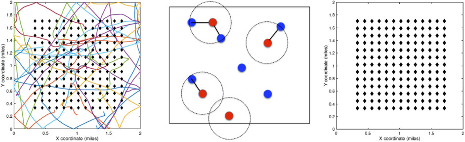
FIGURE 1. Left: random walk model for agent motions. Middle: proximity-based spread of infections from infected to susceptible agents. Right: layout of households on a square grid in the center of the domain.

An agent’s health situation follows the chart shown on the left side of Figure 2. Susceptible agents become infected when exposed to infected agents, with a certain probability. The infected agents go through a period of sickness, with two eventual outcomes—full recovery for most and death for a small fraction. That is, one starts as noninfected or susceptible, potentially gets infected with a certain probability, and later recovers or dies according to their event probabilities. Those with nonfatal infections are further labeled as symptomatic or asymptomatic agents. Naturally, agents with fatal outcomes are labeled as symptomatic. This labeling allows for the selective imposition of lockdown measures on a subset of the population. Once recovered, we assume that the agents can no longer be infected, as suggested by the CDC FAQ [16]. The social dynamical model used here is based on a fixed domicile, that is, each agent has a fixed housing unit. Under unrestricted conditions, that is, no lockdown, the agents are free to move over the full domain using a simple motion model. These motions are independent across agents and encourage smooth paths. Under lockdown conditions, the required agents head directly to their housing units and generally stay there during that period. The remaining agents, including a small fraction of agents, termed essential workers, are allowed to move freely under the restrictions. The infected agents under lockdown can only infect other susceptible agents living in the same household and not the general public, as shown on the right side of Figure 2. Similarly, mobile infected agents can only infect other mobile agents but not those under the lockdown. Three types of lockdowns are considered: 1) lockdown of the full population or LD1, 2) lockdown of infected agents or LD2, and 3) lockdown of symptomatic agents or LD3.

FIGURE 2

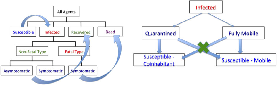
FIGURE 2. Left: flow chart for evolution of infection dynamics for the population. Right: scheme for infection of susceptible agents from infected agents.

The main highlights and contributions of this article are as follows: 1) agent-level transmission of infections and thus, a more granular analysis than (population-level) deterministic dynamical models, 2) random-walk motions of agents when unconstrained and restricted to households when under lockdowns, 3) different classifications of infections: fatal and nonfatal, with the latter being either symptomatic or asymptomatic, 4) selective lockdowns for different strata of the population, and 5) statistical quantifications of gains resulting from lockdown restrictions and their timings on infection rates.

The rest of this article is as follows. Random-Walk, Agent-Level Pandemic Simulation (RAW-ALPS) develops the proposed RAW-ALPS model, specifying the underlying assumptions and motivating model choices. It also discusses choices of model parameters and provides comparisons with the SIRD model. Exemplar Outcomes and Computational Cost presents some illustrative examples and discusses the computational complexity of RAW-ALPS, while Analyzing Effects of Lockdown Measures develops the use of RAW-ALPS in understanding the influences of countermeasures. The article ends by discussing model limitations and suggesting some future directions.

2 Random-Walk, Agent-Level Pandemic Simulation (RAW-ALPS)

In this section, we develop our simulation model for agent-level interactions and the spread of the infections. For this, we consider a population in a predetermined geographical domain. In terms of the model design, there are competing requirements for such a simulation to be useful. On the one hand, we want to capture detailed properties of agents and their pertinent environments, to render a realistic scenario for pandemic evolution. On the other hand, we want to keep model complexity reasonably low, to utilize it for analyzing variable conditions and countermeasures. Also, to obtain statistical summaries of pandemic conditions under different scenarios, we want to run a large number of simulations and compute averages. This process also requires keeping the overall model simple, from a computational perspective, to allow for multiple runs of RAW-ALPS.

2.1 Simplifying Assumptions

The overall setting of the simulation model is as follows. We assume that the community is located in a square geographical region D with h household units arranged centrally on a uniformly spaced square grid in D (see the right panel of Figure 1). We assume that there is a fixed number, say N, of total agents in the community (including all classifications—uninfected, infected, dead, etc.) and their health status updates every unit interval (e.g., 1 h), indexed by variable t. The unconstrained agents can traverse freely through all parts of D but are largely restricted to their home units under restrictions. Next, we specify some simplifying assumptions:

• Independent Agents: An agent’s movements and infection status are independent of those of other agents. The actual infection event is, of course, dependent on one being in close proximity to an infected carrier (within a certain distance, say ≈ 6 feet) for a certain exposure time. But the probability of an agent being infected is independent of such events for other agents.

• Full Mobility in Absence of Restrictive Measures: As mentioned above, we assume that each agent is fully mobile and moves across the domain freely when no restrictive measures have been imposed. In other words, there is no effect of an agent’s age, gender, or health on his/her mobility. Also, we do not impose any day/night schedules on the motions. Some articles, including [17], provide two- or three-state models where the agents transition between some stable states (home, workplace, shopping, etc.) in a predetermined manner. To implement such detailed models requires careful considerations about the daily movement patterns of agents, and that increases model complexity.

• Homestay During Restrictive Measures: We assume that most agents comply with instructions and stay at home at all times during the lockdown conditions. Only a small percentage (set as a parameter ${\rho }_0$) of the population, representing essential workers, are allowed to move freely, but a large majority stays at home.

• Sealed Region Boundaries: In order to avoid complications resulting from a transportation model in the system, we assume that there is no transfer of agents into and out of the region D. The region is modeled to have reflecting boundaries to ensure that all citizens stay within the region. The only way the population of D can be changed is through death.

• Fixed Domicile: The whole community is divided into a certain number of living units (households or buildings). These units are placed in square blocks with uniform spacing. Each agent has a fixed domicile at one of the units. During a lockdown period, the agents proceed to and stay at home with a high compliance level. We assume that all agents within a domicile unit are exposed to each other, that is, they are in close proximity and can potentially infect others.

• No Reinfection: We assume that once a person has recovered from the disease, he/she cannot be infected again for the remaining observation period. While this is an important unresolved issue for the current COVID-19 infections, it has been a valid assumption for the past coronavirus infections and it remains the current CDC guideline [16].

• Single Patient Ground Zero: The infection is introduced in the population using a single carrier, termed patient ground zero at time t = 0. This patient is selected randomly from the population and the time t is measured relative to this initial event.

• Constant Immunity Level: The probability of infection of agents, under the exposure conditions, remains the same over time. We do not assume any increase or decrease in an agent’s immunity level over time. Also, we do not assign any age or ethnicity to the agents and all agents are assumed to have equal immunity levels.

2.2 Model Specifications

There are several parts of the model that require individual specifications. These parts include modeling the movements of each agent (with or without restrictions in place), the mechanisms of transmitting infections from agent to agent, and the processes of recovery and fatality for infected agents. A full listing of the model parameters and some typical values are given in Table A1 in the Appendix.

• Motion Model: The movement of an agent follows a simple random-walk model where the instantaneous velocity $v_i\left(t\right)$ is a weighted sum of three components: 1) velocity at the previous time, that is, $v_i\left(t\mathrm{-}1\right)$, 2) a directed component guiding them to their home, $\left(h_i\mathrm{-}{x}_i\left(t\mathrm{-}1\right)\right)$, where $x_i\left(t\right)$ is the agent location at time t, and 3) an independent Gaussian increment $\sigma w_i\left(t\right)$, $w_i\left(t\right)\sim \mathcal{N}\left(\mathrm{0,1}\right)$. Note that the motions of different agents are kept independent of each other. The location $h_i\mathrm{\in }D$ denotes the home unit (or stable state) of the $i^{th}$ agent.

Using mathematical notation, the model for instantaneous position $x_i\left(t\right)$ and velocity $v_i\left(t\right)$ of the $i^{th}$ agent are given by

$\begin{array}{l}{v}_i\left(t\right)=\mu v_i\left(t-1\right)+\alpha \left(1-\mu \right)\left(h_t-x_i\left(t-1\right)\right)+\sigma w_i\left(t\right),0\le \mu \le 1,\\ x_i\left(t\right)=x_i\left(t-1\right)+\delta v_i\left(t\right).\end{array}(2)$

Here $\alpha \mathrm{\in }{\mathrm{ℝ}}_{\mathrm{+}}$ determines how fast one moves toward their home and µ quantifies the degree to which one follows the directive to stay home. When $\mu \mathrm{=}0$, an agent reaches home and stays there, except for a random perturbation $w_i$. However, if $\mu \mathrm{=}0.5$, then a significant fraction of motion represents continuity in velocity, irrespective of the home location. The value $\mu \mathrm{=}1$ implies that either there is no lockdown or the agent does not comply with the directive.

Reflecting Boundaries: When a subject reaches the boundary of the domain D, the motion is reflected, and the motion continues in the opposite direction.

Figure 3 shows examples of random agent motions under different simulation conditions. The leftmost panel shows a situation with no lockdown and the agents are moving freely according to Eq. 2. The middle panel shows the case where the restrictions are imposed on Day 10 and stay in place after that. The last panel shows the case where a lockdown is imposed on Day 10 and then lifted on Day 20. The blue curves represent free motion before a lockdown, the red denotes motion toward home during a lockdown, and the green represents free motion again after the lockdown is lifted.

• Lockdown Model: Once the lockdown starts, at time say $T_0$, agents are directed toward their homes and asked to stay there. We assume that $\rho \mathrm{\%}$ of the subjects follow this directive, while the others $\left(\left(100\mathrm{-}\rho \right)\text{\%}\right)$ follow a different motion model. The variable ρ changes over time according to

$\rho \left(t\right)=\{\begin{array}{ll}0,\hfill & t<T_0\left(\text{under no restrictions}\right)\hfill \\ {\rho }_0,\hfill & t\ge T_0\left(\text{under restrictions}\right)\hfill \end{array},$

where ${\rho }_0$ is set to be a large number: 98% or 99%. We note that the people who do not follow restrictions follow the prescribed motion model Eq. 2 with $\mu \mathrm{=}1$. We study three types of lockdowns in this article: 1) lockdown of the full population, termed LD1, 2) lockdown of infected agents, termed LD2, and 3) lockdown of symptomatic agents, termed LD3.

• Exposure–Infection Model: Infection of a susceptible agent depends on the level of exposure to an infected agent, irrespective of the infected agent being symptomatic or not. Recall that mobile infected agents can only infect other mobile agents, while agents in a lockdown can only infect agents in the same household. To create the conditions for the spread of infection:

 • The physical distance between the susceptible agent and the infected agent during exposure should be less than $r_0$.

 • The exposure time in terms of the time units is at least ${\tau }_0$. In this study, we use the cumulative time exposure for an agent over the whole history, rather than just the recent history.

 • Under these conditions, the probability of being infected at each time t is an independent Bernoulli random variable with probability $p_I$.

• Recovery–Death Model: Once a subject is infected, we randomly assign a label or infection type immediately. Either an infected agent is going to recover (nonfatal type, or NFT) or the person is eventually going to die (fatal type, or FT). The probability of having a fatal type, given that a person is infected, is $p_F$. An agent with the NFT label is further classified as either Symptomatic (S) or Asymptomatic (AS) with a certain probability $p_S$. All agents with the FT label are classified as symptomatic.

• Recovery: An agent with a nonfatal type (NFT) is sick for a period of $T_R$ days. After this period, the person can recover at any time, according to a Bernoulli random variable with probability $p_R$ in each time step.

• Fatality: An agent with a fatal type (FT) is sick for a period of $T_D$ days. After this period, the person can die at any time, independently according to a Bernoulli random variable with probability $p_D$.

FIGURE 3

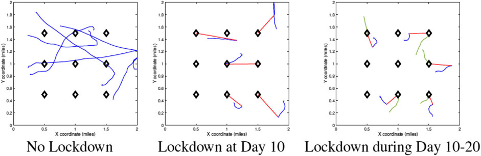
FIGURE 3. Sample agent motions under different conditions. Blue curves denote unrestricted movements, red curves denote movement toward home units during a lockdown, and green curves denote movement after lockdown.

2.3 Chosen Parameter Values

A complete listing of the ALPS model parameters is provided in Appendix Table A1. In this section, we motivate the values chosen for those parameters in these simulations. We justify these choices from the current reports of the COVID-19 pandemic. As argued in [18], a realistic choice of parameters is very important in establishing the validity of simulation models.

• Population Density: We use a square domain D of size $2\mathrm{\ast }2$ miles² or $\mathrm{5\ast 5}$ miles² for a community with a population of N agents. The value of N changes in different experiments. The values of $N\mathrm{=}900$ and $D\mathrm{=}{\left[\mathrm{0,2}\right]}^2$ represent a population density of 225 people/mile². The community contains h living units (buildings) with a domicile of $N/h$ people per unit. In case $N/h$ is high ($\approx 100$), a unit represents a tall building in metropolitan areas, but when $N/h$ is small ($\approx 5$), a unit represents a single-family home in a suburban area.

The time unit for updating configurations is 1 h and the occurrence of major events is specified in days. For example, the lockdown can start on Day 1 and end on Day 30.

• Agent Speeds: The standard deviation for accelerations, denoted by σ, in agent mobility are approximately 1–5 feet/h (fph). Through integration over time, this results in agent speeds up to 1,000 fph. We assume that ${\rho }_0\mathrm{=}0.9\mathrm{-}0.98$, that is, 90–98% of the people follow the restriction directives.

• Infection Rates: The physical distance between agents to catch infection should be at most $r_0\approx 6\text{ft}$ and the exposure time should be at least ${\tau }_0\mathrm{=}5$ time units (hours). The probability $p_I$ of getting infected, under the right exposure conditions, is set at 5% at each time unit (hour) independently. There is no current reference literature on selecting this value since it is difficult to measure precise exposure events for people who have tested positive for COVID-19. While contact tracing [19] is being developed to ascertain infection rates, there are no public data currently available to measure this infection rate. This value leads to overall infection rates that are similar to national and international infection rates [20].

• Fatality Rate: Once infected, the probability of having a fatal outcome is set at 5–10%, according to the mortality rate listed by the CDC [21]. The period of recovery for agents with nonfatal outcomes starts at 7 days. The probability of reaching full recovery for those agents is $p_R\mathrm{=}0.001$ at each subsequent time unit (hour). Similarly, for the agents with fatal outcomes, the period of being infected is set to be 7 days and after that, the probability of death at each time unit (hour) is set to be $p_D=0.1$.

• Asymptomatic Infected Agents: The percentage of infected agents who remain asymptomatic is set to be in the range of 15–40% [22, 23]).

Figure 1 provides a pseudocode for the RAW-ALPS algorithm.

ALGORITHM 1

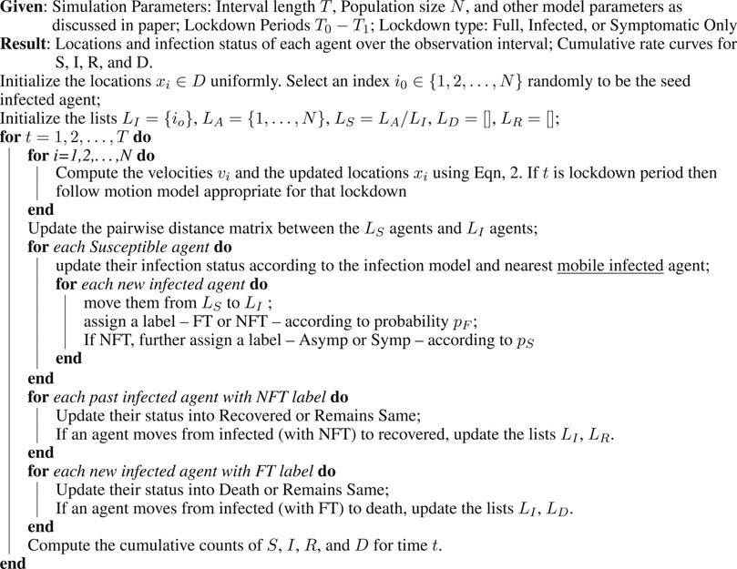
Algorithm 1. RAW-ALPS Pseudocode

2.4. Model Validation

Although RAW-ALPS is perhaps too simple model to capture the intricate dynamics of an actual active society, it does provide an efficient tool for analyzing effects of countermeasures during the spread of a pandemic. Before it can be used in practice, there is an important need to validate it in some way.

As described in Ref. [4], there are several ways to validate a simulation model. One is to use real data (an observed census of infections over time) in a community to estimate model parameters, followed by a statistical model testing. While such data may emerge for COVID-19 in the future (especially with the deployment of tracking apps in many countries), there are currently no such agent-level data available for COVID-19. The other approach for validation is to consider coarse population-level variables and their dynamics and compare them against established models such as SIR and its variations. We will perform validation of RAW-ALPS in two ways.

2.4.1. Qualitative Comparisons with SIR Model

As the first comparison, we study shapes of infection curves resulting from the RAW-ALPS model and compare them qualitatively to the shapes resulting from the SIR model. Figure 4 shows plots of the evolutions of global infection counts (susceptible, infected, and recovered) in a community under the well-known SIR model (on the left) and the proposed ALPS model (on the right). In the ALPS model, the counts for recovered and fatalities are kept separate, while in the SIR model, these two categories are combined. One can see a remarkable similarity in the shapes of the corresponding curves, and this provides a certain validation to the RAW-ALPS model. In fact, given the dynamical models of agent-level mobility and infections, one can derive the parameters of the population-level differential equations used in the SIRD model. We pursue this topic in the next section.

FIGURE 4

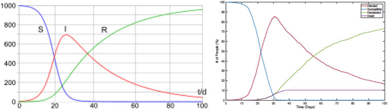
FIGURE 4. Evolution of population-level infection measurements under a typical SIR model (left) (source: Wikipedia) and the RAW-ALPS model (right). Visually, the RAW-ALPS model can generate infection curves with shapes similar to those of the SIR model.

2.4.2 Estimation of SIRD Parameters

In this section, we use data simulated from RAW-ALPS to fit the SIRD model given in Eq. 1 and use estimated SIRD model parameters to provide interpretations. Rearranging equations in the SIRD model (Eq. 1), we get the instantaneous values of the parameters:

$\mu \left(t\right)=\frac{D^{\text{′}}\left(t\right)}{I\left(t\right)},\gamma \left(t\right)=\frac{R^{\text{′}}\left(t\right)}{I\left(t\right)},\beta \left(t\right)=-N\frac{S^{\text{′}}\left(t\right)}{I\left(t\right)S\left(t\right)}=N\frac{I^{\text{′}}\left(t\right)+\gamma I\left(t\right)+\mu I\left(t\right)}{I\left(t\right)S\left(t\right)}.$

Let $1_{f\mathrm{(}t\mathrm{)}>0}$ denote the domain over which a function $f\left(t\right)$ is strictly positive. We define the estimators of overall SIRD parameters to be

$\begin{array}{l}\widehat{\mu }=\text{mean}\left(\frac{D^{\text{′}}\left(t\right)}{I\left(t\right)}{1}_{I\left(t\right)>0}\right),\widehat{\gamma }=\text{mean}\left(\frac{R^{\text{′}}\left(t\right)}{I\left(t\right)}{1}_{I\left(t\right)>0}\right),\\ \widehat{\beta }=\frac{N}{2}\text{mean}\left(\frac{1_{I\left(t\right)S\left(t\right)>0}}{I\left(t\right)S\left(t\right)}\left(I^{\text{′}}\left(t\right)+\gamma I\left(t\right)+\mu I\left(t\right)-S^{\text{′}}\left(t\right)\right)\right).\end{array}$

Since in our simulations we have a small population size (N), the number of dead agents becomes a constant soon after any changes are complete, making $D^{\text{′}}\mathrm{(}t\mathrm{)=}0$ for most of the study. To focus on the mortality rate in the active period, we modify the estimator of µ to be$\widehat{\mu }=\text{mean}\left(\frac{D^{\text{′}}\left(t\right)}{I\left(t\right)}{1}_{D^{\text{′}}\left(t\right)I\left(t\right)>0}\right)$.

Figure 5 shows an example of this estimation using data simulated from RAW-ALPS for an unrestricted situation. The left plot shows the evolution of $S/I$ functions under the chosen simulation parameters. The infection reaches its peak around Day 26 and there are no uninfected agents left after that. For these data, the estimated values of parameters are $\widehat{\beta }=0.036281$, $\widehat{\gamma }=0.000860$, and $\widehat{\mu }=0.001005$ (at hourly unit time). We clarify that the simulation is updated at an hour unit, but the final estimates of these rates are converted into daily time unit to compare with published values. The basic reproduction number for this simulation comes out to be $R_0\mathrm{=}\frac{\widehat{\beta }}{\widehat{\gamma }}\mathrm{=}42.1703$.

FIGURE 5

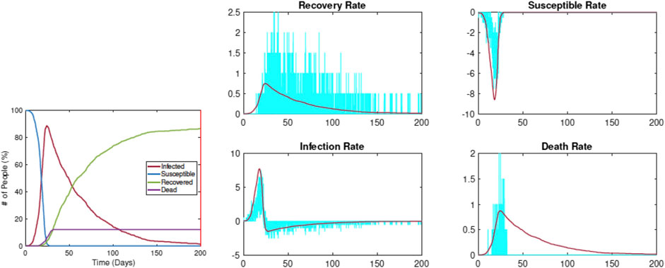
FIGURE 5. Estimation of SIRD parameters from data simulated by RAW-ALPS for an unconstrained spread. The pandemic curves generated by the SIRD model with estimated parameters match the RAW-ALPS output.

Figure 6 shows when the restrictions are imposed on Day 5. The left plot shows the evolution of $S/I$ functions—the infection reaches its peak around Day 20 even though there is a significant portion of uninfected agents. For these data, the estimated values of parameters are $\widehat{\beta }\mathrm{=}0.002860$, $\widehat{\gamma }=0.001005$, and $\widehat{\mu }=0.002459$ (at hourly unit time). The basic reproduction number for this simulation comes out to be $R_0=\frac{\widehat{\beta }}{\widehat{\gamma }}=2.8458$.

FIGURE 6

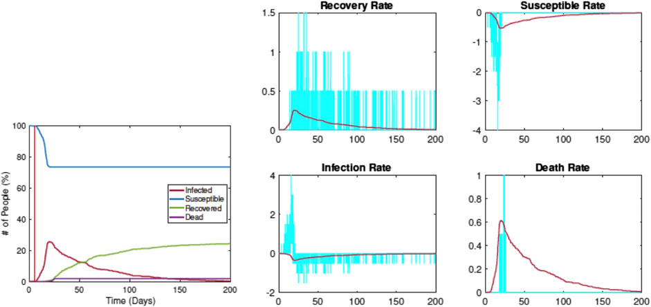
FIGURE 6. Estimation of SIRD parameters from data simulated by RAW-ALPS for the case when the restrictions are imposed on Day 5. Once again, the pandemic curves generated by the SIRD model with estimated parameters match the RAW-ALPS output.

Compared with the previous example, we see that the infection rate comes down significantly, from $\widehat{\beta }=0.036281$ to $\widehat{\beta }=0.002860$, when the restrictions are imposed. Similarly, the reproduction number also comes down from 42.1703 to 2.8458.

3 Exemplar Outcomes and Computational Cost

We illustrate the use of the RAW-ALPS model by presenting some sample outcomes under some typical scenarios. Furthermore, we discuss the computational cost of running RAW-ALPS on a laptop computer.

3.1 Examples From RAW-ALPS

We start by showing sample outputs of RAW-ALPS under some interesting settings. In these examples, we use a relatively small number of agents ($N=1500$) and household units ($h=289$), with $T=50$ days, in order to improve visibility of displays.

1. Example 1—No Restrictive Measures: Figure 7 shows a sequence of temporal snapshots representing the community at different times over the observation period. In this example, the population is fully mobile over the observation period and no social distancing restrictions are imposed. The snapshots show the situations on Day 8, 17, 33, and 42. The corresponding time evolutions of global count measures $[S\mathrm{(}t\mathrm{)},I\mathrm{(}t\mathrm{)},D\mathrm{(}t\mathrm{),}\text{and}R\mathrm{(}t\mathrm{)}]$ are shown in the bottom right panel. The infection starts to spread rapidly around Day 5 and reaches a peak infection level of 78% around Day 17. Then, the recovery starts and continues until very few infected people are left. In this simulation, the number of fatalities is found to be 6%.

2. Example 2—Early Restrictions: In the second example, a lockdown of all the infected agents is introduced on Day 5 and these measures stay in place after that. The results are shown in Figure 8. Once again we show snapshots for situations on Day 8, 17, 33, and 42. The corresponding time evolutions of global count measures are shown in the bottom right panel. As the summary shows, an early restriction of lockdown is very effective in controlling the spread of the infection and the peak infection rate is minuscule at 3%.

3. Example 3—Early Restrictions but Removed Later: In the next example, a full lockdown or LD1 is introduced on Day 2 but removed on Day 30. The results are shown in Figure 9. In early snapshots, the population is under a lockdown and the spread is minimal. By Day 33, the lockdown is released, and the population is fully mobile. Consequently, the infection begins to spread again, and by Day 42, the infection reaches its peak value.

4. Example 4—Delay in Imposing Restrictions: In the last example, with results shown in Figure 10, a full lockdown (LD1) is introduced very late (on Day 10). In this simulation run, the infection rate reaches a peak value of 80% despite a lockdown. This is because the infection had already spread extensively in the population by the time the lockdown starts.

FIGURE 7

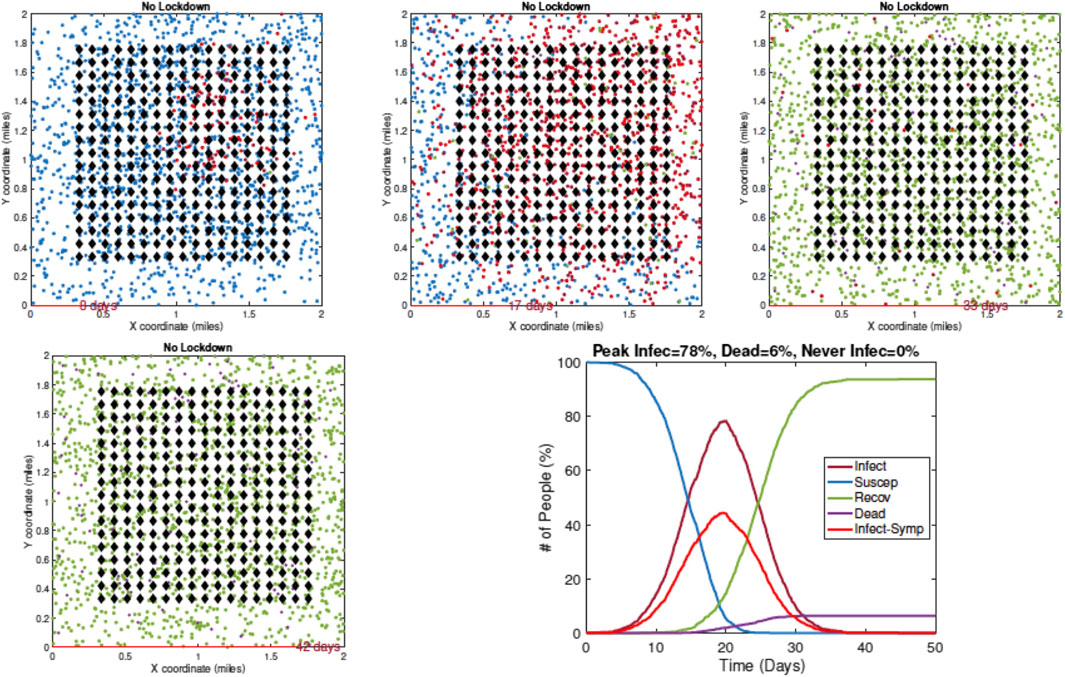
FIGURE 7. Example 1: model outputs at different times under no restrictive measures. Blue dots are susceptible agents, red dots are infected agents, green dots are recovered agents, and purple circles denote fatalities. The pandemic curves in the bottom right exhibit typical behavior of the RAW-ALPS model at the population level.

FIGURE 8

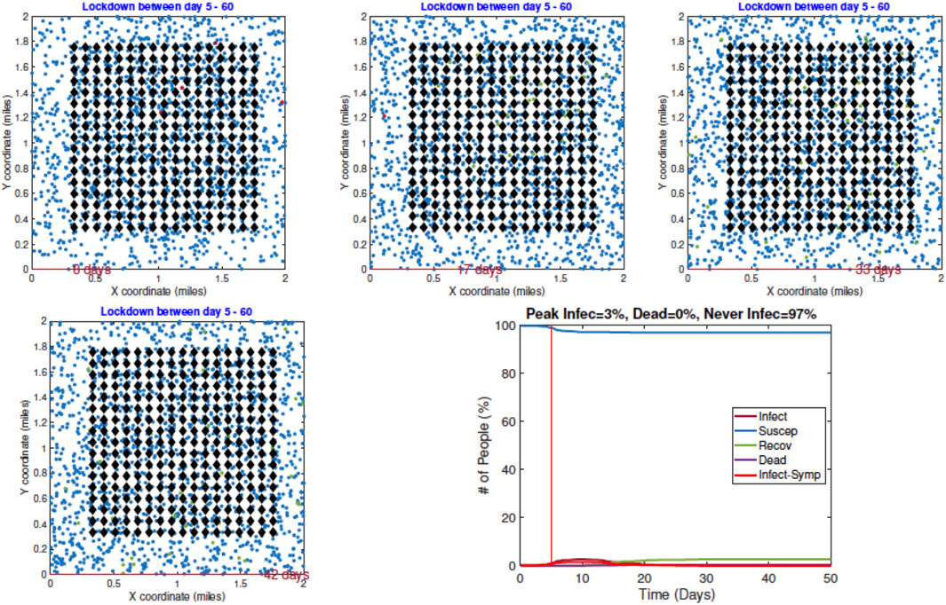
FIGURE 8. Example 2: displays of model outputs when a lockdown of infected people (LD2) is imposed on Day 5. The pandemic curves in the bottom right show a drastic reduction in infection due to the lockdown.

FIGURE 9

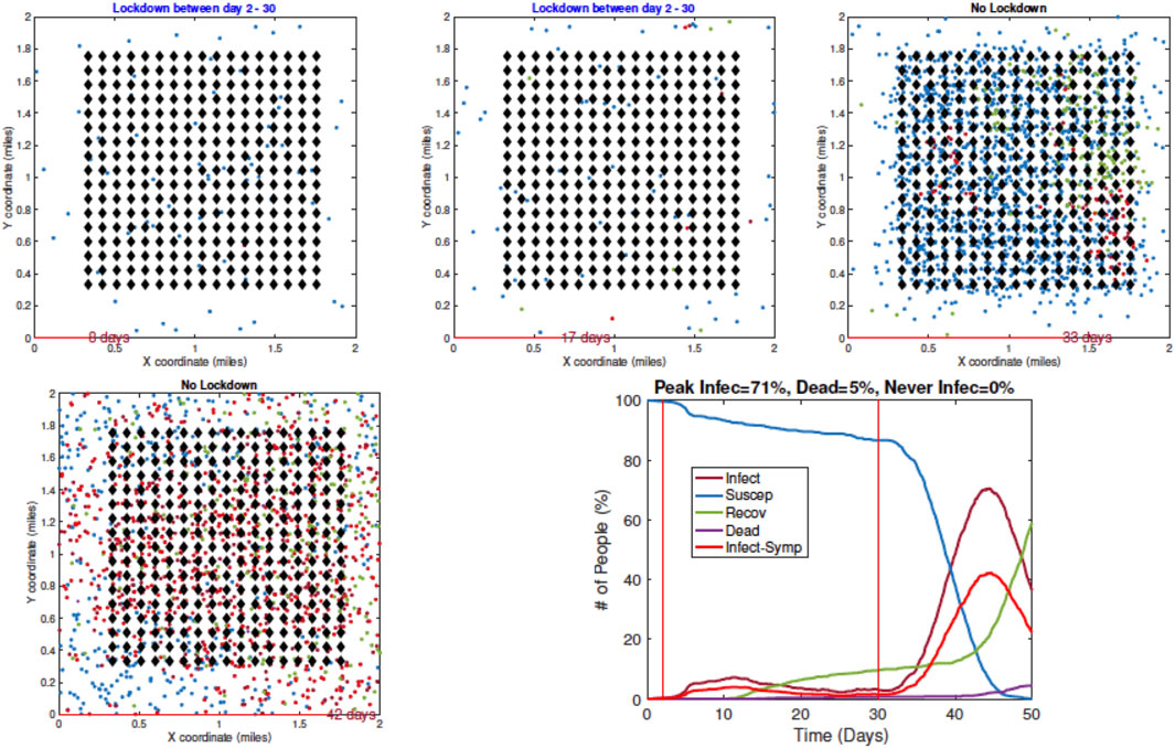
FIGURE 9. Example 3: model outputs when a full lockdown or LD1 is imposed on Day 2 and removed on Day 30. As seen in the plot of the resulting pandemic curves, the infection is controlled at first by the lockdown, but it spreads fast after the lockdown is lifted.

FIGURE 10

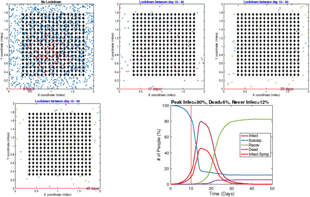
FIGURE 10. Example 4: model outputs when a full lockdown is imposed on Day 10. The pandemic curves show that the infection has spread widely in the community by the time a lockdown is imposed.

3.2. Computational Complexity

The main computational cost in the simulation comes from the need to update the following variables at each time t:

• locations of all agent according to their independent motion model;

• pairwise distance matrix between Susceptible agents and Infected agents; and

• infection status of each agent according to the infection dynamics.

In general, we obtain some efficiency by performing matrix operations, rather than using “for loops” for these updates across agents. Additionally, we increase speed by maintaining a list of neighborhoods for each agent and checking interactions only between the neighbors at each t.

Since the computational efficiency of the simulator is of vital importance, we study the computational cost of running RAW-ALPS for different variable sizes. In these experiments, we note the time taken by RAW-ALPS code on a MacBook Pro laptop with an Intel 2.8 GHz Core i7 processor and 16 GB memory. In Figure 11 we plot average run times (using five runs in a setting) of the code for different values of N, h, and T. Recall that h is the number of household units, N is the number of agents, and T is the period length. From these results, we see that the computational cost is linear in T, which makes sense. The computational cost is superlinear in N, keeping other variables fixed. This is because an increase in N represents a higher density and increased infection rates, thus requiring additional computations for tracking infected agents. Interestingly, for the range of parameter values studied here, the computational cost does not grow with an increase in h. As an aside, we note that for $N=5000$ and $h=1521$, the run time for $T=100$ days is approximately 330 s and for $T=150$ days is approximately 484 s.

FIGURE 11

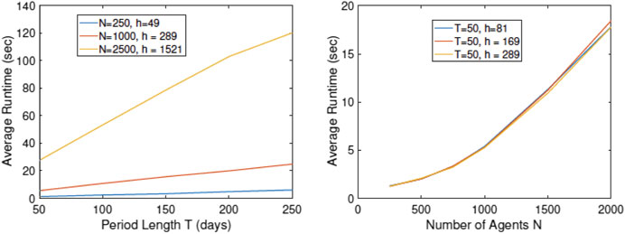
FIGURE 11. Plots of run times vs. simulation parameters T, N, and h. The algorithmic cost is linear in T but superlinear in N.

4 Analyzing Effects of Lockdown Measures

There are several ways to utilize this model for prediction, planning, and decision-making. We illustrate some of these ideas using examples.

4.1 Timing of Imposition of Full Lockdown

First, we study the effect of time of a full lockdown on the epidemic infections. In the following simulations, we have used $N=1000$ agents with $h=361$ households in the scene domain ${\left[\mathrm{0,2}\right]}^2$ miles. For the infection parameters, we use a contact radius $r_0=0.02$ miles, contact period ${\tau }_0=5\text{h}$, and $p_I=0.1$. The motion parameters are: $\sigma =0.0002\text{mph}$, $\mu =0.02$, and $\alpha =0.1$. In each setting, we run the code 30 times and collect the simulation outputs.

Figure 12 shows examples of RAW-ALPS outputs when we impose a full lockdown on the community but at different times. From top to bottom, the plots show lockdowns starting on Day 2, Day 10, and Day 30, respectively, with the last row showing results for no lockdown. Once the restrictions are imposed, they are not removed in these examples. As expected, the best results are obtained for the earliest imposition of restrictions. In the case of no lockdown, the peak infection rate in the population ranges from 60 to 80%, which is very high for a community. The fraction of fatalities ranges from 6 to 8%, and the fraction of community that is never infected is zero in all runs. In case the restrictions are imposed on Day 2, with all other parameters held the same, there is a remarkable improvement in the situation. The peak infection goes down to 2–3%, the fatalities decrease to 0.1–0.2%, and the fraction of uninfected goes up to 98–99%. Thus, an early imposition of full lockdown measures helps significantly reduce infection in the community.

FIGURE 12

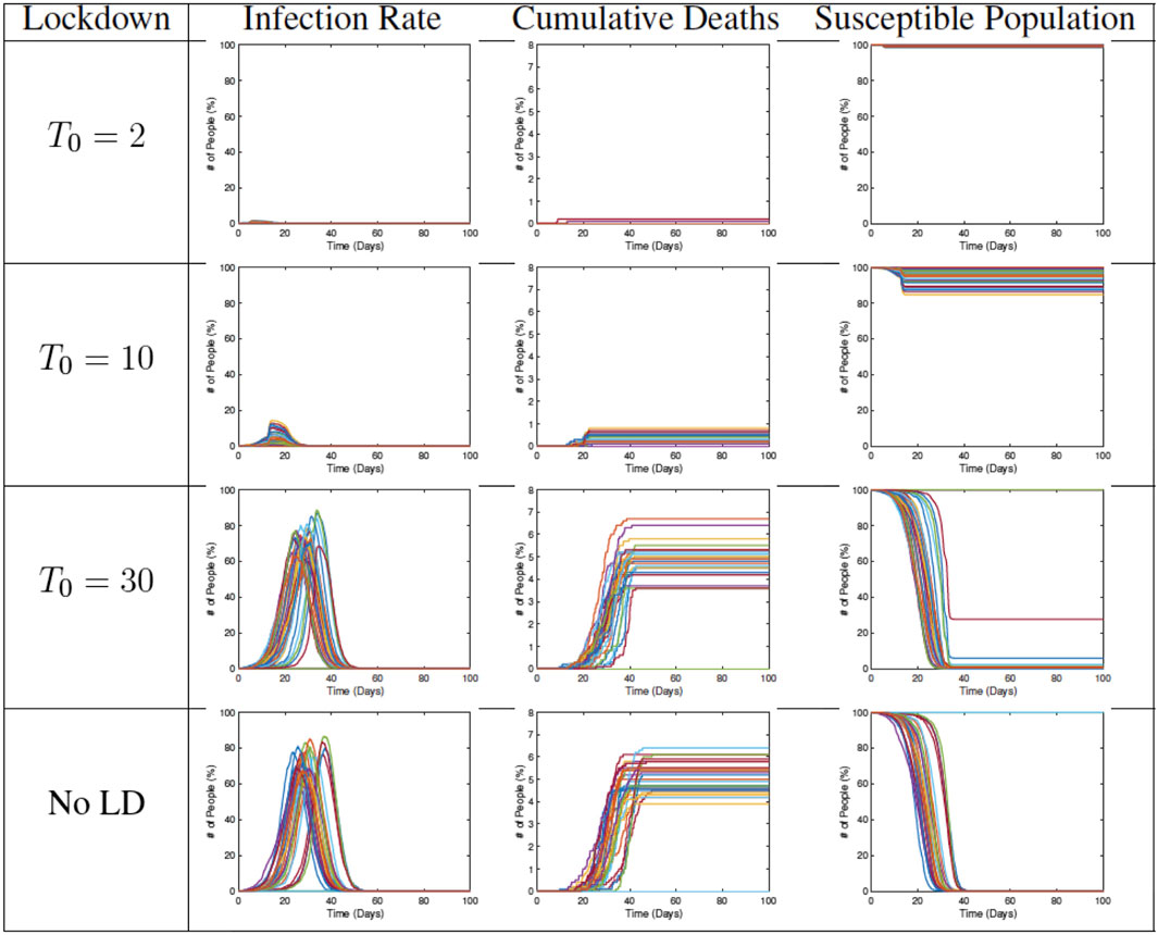
FIGURE 12. Results from RAW-ALPS runs for a full lockdown (LD1) starting at different times. Going from top to bottom, we impose lockdowns later and later. The effect of a lockdown diminishes significantly if the start of the lockdown is delayed.

4.2 Timing of Removal of Restrictions

In the next set of simulations, we study the effects of lifting restrictions and thus re-allowing full mobility in the community. Some sample results are shown in Figure 13. Each plot shows the evolution for a different end time $T_1$, while the start time is kept fixed at $T_0=5$. As these plots indicate, the gains made by early imposition of restrictions are nullified when the restrictions are lifted too soon. In the case of early lifting of restrictions, the full population gets infected eventually. Since we do not assume any change in the immunity levels of the agents over time, the results from early lifting of restrictions are quite similar to those from not imposing any restrictions in the first place. The results appear to be the same, just shifted in time.

FIGURE 13

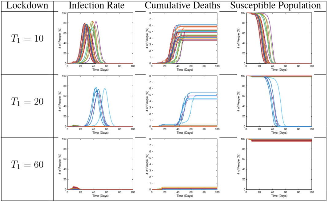
FIGURE 13. Results from RAW-ALPS runs for a full lockdown (LD1) ending at different times. Going from top to bottom, we keep the lockdowns for longer periods. A longer imposition of lockdown helps in reducing the spread of the epidemic.

4.3 Statistical Summaries

In the next set of experiments, we compute average values of some variables of interest using 30 runs of RAW-ALPS. In the first result, we study three variables—number of deaths, number of agents remaining uninfected, and the peak infection rate—using $N=1000$ agents living in a community of $h=361$ households, observed over $\left[\mathrm{0,100}\right]$ days. We vary the start time $T_0$ (start day of restrictions) from 2 to 30 and then to 100 and study the resulting outcomes. (The value of $T_0=100$ implies that the restrictions are never imposed in that setting.)

Figure 14 shows box plots of these three variables against $T_0$, with each row representing a different type of lockdown. The first column shows the median percentage of fatalities in the population for different lockdown types. The second column shows the fraction of the uninfected population and the last column shows the peak infection rates. It can be seen that the results are very similar for a full lockdown (LD1) and a lockdown of infected agents (LD2) but are quite different for a lockdown of only the symptomatic agents (LD3). We find that this last type of lockdown is ineffective in containing the spread of the infection, except for when $T_0\mathrm{=}2$. These results suggest that a lockdown of only the infected agents (LD2) can be an effective strategy in controlling the epidemic. Of course, given the asymptomatic nature of the disease, it is not possible to ascertain the infection status precisely. One can only estimate this status for a large population using accurate and extensive testing schemes.

FIGURE 14

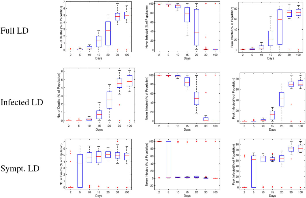
FIGURE 14. Statistical summaries of infection variables obtained using 30 runs of RAW-ALPS, plotted against the starting day of the lockdown. In all three lockdown types, a delay in imposing lockdown causes an increase in infections and casualties.

In Figure 15, we study the impact of changing $T_1$ while $T_0\mathrm{=}1$ is kept fixed (and other experimental conditions being the same as in the last experiment). The three panels show the fractions of deaths (left), the number of uninfected (middle), and the peak infection rates (right). Each curve in the panel corresponds to a different lockdown type: full LD or LD1, infection LD or LD2, and symptomatic LD or LD3. The results show that for LD1 and LD2, a delay in the lifting of the restrictions is effective in controlling the epidemic. In contrast, the imposition of LD3 is not as effective. Interestingly, these results show that LD2 is more effective than LD1. This may be because in full lockdown, the chances of susceptible agents coinhabiting with the infected agents increase and this, in turn, increases the infection rates.

FIGURE 15

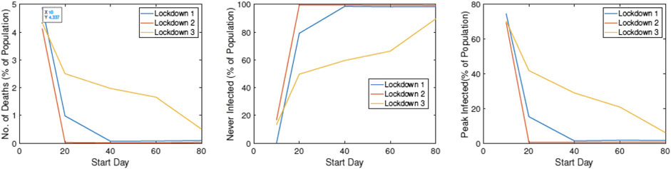
FIGURE 15. Statistical summaries of infection variables obtained using 30 runs of ALPS, plotted against $T_1$, the reopening day. In all three types of lockdowns, a delay in reopening after a lockdown helps control the number of infections and deaths.

5 Discussion and Conclusion

This article develops an agent-based simulation model, called RAW-ALPS, for modeling the spread of an infectious disease in a closed community. Several simplifying yet reasonable assumptions make RAW-ALPS efficient and effective for statistical analysis. The model is validated at a population level by comparing it with the popular SIR model in epidemiology.

The results from RAW-ALPS show that a lockdown of only the infected agents (LD2) is the most effective kind. However, this includes both symptomatic and asymptomatic agents, with the latter ones not being easy to detect. This calls for regular and extensive testing of the population to isolate and restrict all infected agents while allowing for free movements of all uninfected agents. Furthermore, these results indicate that 1) early imposition of lockdown measures (right after the first infection) significantly reduces infection rates and fatalities; 2) lifting of lockdown measures recommences the spread of the disease, and the infections eventually reach the same level as that of the unrestricted community; and 3) in the absence of any extraneous solutions (a medical treatment/cure, a weakening mutation of the virus, or natural development of agent immunity), the only viable option for preventing large infections is the judicious use of lockdown measures.

The strengths and limitations of the RAW-ALPS model are the following. It provides efficient yet comprehensive modeling of the spread of infections in a self-contained community, using simple model assumptions. The model can prove very useful in evaluating costs and effects of imposing different types of social lockdown measures in a society. In the current version, the initial placement of agents is set to be normally distributed with means given by their home units and fixed variance. This variance is kept large to allow for near arbitrary placements of agents in the community. In practice, however, agents typically follow semirigid daily schedules of being at work, performing chores, or being at home. Thus, at the time of imposition of a lockdown, the agents can be better placed in the scenes according to their regular schedules, rather than being placed arbitrarily.

In terms of future directions, there are many ways to develop this simulation model to capture more realistic scenarios. 1) It is possible to model multiple, interactive communities instead of a single isolated community. 2) One can include typical daily schedules for agents in the simulations. A typical agent may leave home in the morning, spend time at work during the day, and return home in the evening. 3) It is possible to provide age demographics to the community and assign immunity to agents according to their demographic labels [24]. 4) As more data becomes available in the future, one can change immunity levels of agents over time according to the spread and seasons. 5) In practice, when an agent is infected, he/she goes through different stages of the disease, associated with varying degrees of mobility [13]. One can introduce an additional variable to track these stages of infections in the model and change agent mobility accordingly. 6) One can incorporate super spreader events in the model to help capture these mechanisms of transmission. 7) Finally, one can use the output of RAW-ALPS, in conjunction with techniques for the analysis of epidemic curves [25–27], to further adapt simulation parameters to a given community or region.

Data Availability Statement

The raw data supporting the conclusion of this article will be made available by the authors, without undue reservation.

Author Contributions

All authors listed have made a substantial, direct, and intellectual contribution to the work and approved it for publication.

Funding

This research was supported in part by the grants NSF DMS-1621787 and NSF DMS-1953087.

Conflict of Interest

The author declares that the research was conducted in the absence of any commercial or financial relationships that could be construed as a potential conflict of interest.

Appendix: listing of alps parameters

Table A1 provides a listing of all the parameters one can adjust in ALPS to achieve different scenarios. It also provides some typical values used in the experiments presented in the article.

TABLE A1

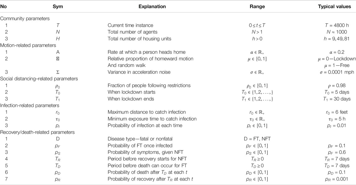
TABLE A1. Listing of parameters associated with different model components of ALPS.

References

1. Bertozzi, AL, Franco, E, Mohler, G, Short, MB, and Sledge, D. The challenges of modeling and forecasting the spread of COVID-19. Proc Natl Acad Sci (2020). 117:16732–16738. doi:10.1073/pnas.2006520117

PubMed Abstract | CrossRef Full Text | Google Scholar

2. Adam, D. Special report: the simulations driving the world’s response to COVID-19. Nature (2020). 580 (7803):316–8. doi:10.1038/d41586-020-01003-6

PubMed Abstract | CrossRef Full Text | Google Scholar

3. Chao, DL, Halloran, ME, Obenchain, VJ, and Longini, JIM. FluTE, a publicly available stochastic influenza epidemic simulation model. Plos Comput Biol (2010). 6:e1000656. doi:10.1371/journal.pcbi.1000656

PubMed Abstract | CrossRef Full Text | Google Scholar

4. Hunter, E, Mac Namee, B, and Kelleher, JD. A taxonomy for agent-based models in human infectious disease epidemiology. J Artif Societies Soc Simulation (2017). 20. doi:10.18564/jasss.3414

CrossRef Full Text | Google Scholar

5. Kermack, WO, and McKendrick, AG. A contribution to the mathematical theory of epidemics. Proc R Soc A (1927). 115:700–721. doi:10.1098/rspa.1927.0118

CrossRef Full Text | Google Scholar

6. Osemwinyen, AC, and Diakhaby, A. Mathematical modelling of the transmission dynamics of ebola virus. Appl Comput Math (2015). 4:313–320. doi:10.11648/j.acm.20150404.19

CrossRef Full Text | Google Scholar

7. Timpka, T, Eriksson, H, Gursky, EA, Nyce, JM, Morin, M, and Jenvald, J. Population-based simulations of influenza pandemics: validity and significance for public health policy. Bull World Health Organ (2009). 87:305–311. doi:10.2471/BLT.07.050203

PubMed Abstract | CrossRef Full Text | Google Scholar

8. Hao, X, Cheng, S, Wu, D, Wu, T, Lin, X, and Wang, C. Reconstruction of the full transmission dynamics of COVID-19 in wuhan. Nature (2020). 584:420–424. doi:10.1038/s41586-020-2554-8

PubMed Abstract | CrossRef Full Text | Google Scholar

9. Verity, R, and Okell, LC, Dorigatti, I, Winskill, P, Whittaker, C, and Imai, N. Estimates of the severity of coronavirus disease 2019: a model-based analysis. Lancet Infect Dis (2020). 20:P669–P677. doi:10.1016/S1473-3099(20)30243-7

PubMed Abstract | CrossRef Full Text | Google Scholar

10. Gilbert, NG. Agent-based models. California, US: Sage Publications (2008).

CrossRef Full Text

11. Epstein, JM, and Axtell, RL. Growing artificial societies Social science from the bottom up. Cambridge, MA: MIT Press (1996).

12. Hunter, E, Namee, BM, and Kelleher, J. An open-data-driven agent-based model to simulate infectious disease outbreaks. PLoS ONE (2018). 13:e0208775. doi:10.1371/journal.pone.0208775

PubMed Abstract | CrossRef Full Text | Google Scholar

13. Perez, L, and Dragicevic, S. An agent-based approach for modeling dynamics of contagious disease spread. Int J Health Geographics (2009). 08:50. doi:10.1186/1476-072X-8-50

PubMed Abstract | CrossRef Full Text | Google Scholar

14. Nguyen, V, Mikolajczyk, R, and Hernandez-Vargas, E. High-resolution epidemic simulation using within-host infection and contact data. BMC Public Health (2018). 18. doi:10.1101/133421

PubMed Abstract | CrossRef Full Text | Google Scholar

15. Silva, PC, Batista, PV, Lima, HS, Alves, MA, Guimaraes, FG, and Silva, RC. COVID-ABS: an agent-based model of COVID-19 epidemic to simulate health and economic effects of social distancing interventions. Chaos Solitons Fractals (2020). 139:110088. doi:10.1016/j.chaos.2020.110088

PubMed Abstract | CrossRef Full Text | Google Scholar

16.Center for Disease Control. Clinical questions about COVID-19: questions and answers (2020). Available at:https://www.cdc.gov/coronavirus/2019-ncov/hcp/faq.html

Google Scholar

17. Dunham, JB. An agent-based spatially explicit epidemiological model in MASON. J Artif Soc Soc Simul (2005). 9:1–3.

Google Scholar

18. Gurdasani, D, and Ziauddeen, H. On fallability of smulations models in informing pandemic responses. Lancet Glob Health (2020). 8:E776–E777. doi:10.1016/S2214-109X(20)30219-9

PubMed Abstract | CrossRef Full Text | Google Scholar

19.Center for Disease Control. Contact tracing resources: resources for conducting contact tracing to stop the spread of COVID-19 (2020). Available at:https://www.cdc.gov/coronavirus/2019-ncov/php/open-america/contact-tracing-resources.html

Google Scholar

20.Covid Volunteer Team. The COVID tracking project (2020). Available at: https://covidtracking.com/

Google Scholar

21.Center for Disease Control. Coronavirus disease 2019 (COVID-19) (2020c). Available at: https://www.cdc.gov/coronavirus/2019-ncov/covid-data/covidview/index.html

Google Scholar

22. Byambasuren, O, Cardona, M, Bell, K, Clark, J, McLaws, M-L, and Glasziou, P. Estimating the extent of asymptomatic COVID-19 and its potential for community transmission: systematic review and meta-analysis. medRxiv (2020). 10.1101/2020.05.10.20097543

Google Scholar

23.Science News. Whole-town study reveals more than 40% of COVID-19 infections had no symptoms (2020). Available from: https://www.sciencedaily.com/releases/2020/06/200630103557.htm (Accessed September 2020).

Google Scholar

24. Chang, SL, Harding, N, Zachreson, C, Cliff, OM, and Prokopenko, M. Modelling transmission and control of the COVID-19 pandemic in Australia. arXiv (2020).

Google Scholar

25. Srivastava, A, and Chowell, G. Understanding spatial heterogeneity of COVID-19 pandemic using shape analysis qof growth rate curves. medRxiv (2020). doi:10.1101/2020.05.25.20112433

CrossRef Full Text | Google Scholar

26. Srivastava, A, and Klassen, E. Functional and shape data analysis. New York, US: Springer (2016).

CrossRef Full Text

27. Srivastava, A, Klassen, E, Joshi, SH, and Jermyn, IH. Shape analysis of elastic curves in Euclidean spaces. IEEE Trans Pattern Anal Mach Intell (2011). 33:1415–1428. doi:10.1109/TPAMI.2010.184

PubMed Abstract | CrossRef Full Text | Google Scholar