 Alexandre Guillet
 Alain Arneodo
 Françoise Argoul
95% of researchers rate our articles as excellent or good
Learn more about the work of our research integrity team to safeguard the quality of each article we publish.
Find out more
ORIGINAL RESEARCH article
Front. Appl. Math. Stat. , 09 April 2021
Sec. Dynamical Systems
Volume 7 - 2021 | https://doi.org/10.3389/fams.2021.624456
This article is part of the Research Topic The New Frontier of Network Physiology: From Temporal Dynamics to the Synchronization and Principles of Integration in Networks of Physiological Systems View all 65 articles
The crosstalk between organs plays a crucial role in physiological processes. This coupling is a dynamical process, it must cope with a huge variety of rhythms with frequencies ranging from milliseconds to hours, days, seasons. The brain is a central hub for this crosstalk. During sleep, automatic rhythmic interrelations are enhanced and provide a direct insight into organ dysfunctions, however their origin remains a difficult issue, in particular in sleep disorders. In this study, we focus on EEG, ECG, and airflow recordings from polysomnography databases. Because these signals are non-stationary, non-linear, noisy, and span wide spectral ranges, a time-frequency analysis, based on wavelet transforms, is more appropriate to handle this complexity. We design a wavelet-based extraction method to identify the characteristic rhythms of these different signals, and their temporal variability. These new constructs are combined in pairs to compute their wavelet-based time-frequency complex coherence. These time-frequency coherence maps highlight the occurrence of a slowly modulated coherence pattern in the frequency range [0.01–0.06] Hz, which appears in both obstructive and central apnea. A preliminary exploration of a large database from the National Sleep Research Resource with respiration disorders, such as apnea provides some clues on its relation with autonomic cardio-respiratory coupling and brain rhythms. We also observe that during sleep apnea episodes (either obstructive or central), the cardiopulmonary coherence (in particular respiratory sinus-arrhythmia) in the frequency range [0.1–0.7] Hz strongly diminishes, suggesting a modification of this coupling. Finally, comparing time-averaged coherence with heart rate variability spectra in different apnea episodes, we discuss their common trait and their differences.
During the past decades, the possibility to capture in real time physiological signals from many tissues (brain, heart, muscles, breath, vessels, intestines, lungs, blood …) has opened new medicine fields, and has brought physicians to a more global view of human beings as complex and multiscale networks of interactions, contributing synergistically to the preservation of health [1–3]. Each organ can be considered as a dynamical system per-se with non-linear and complex oscillations and its interaction with nearby or distant tissues may lead to spatial and/or temporal correlations [4, 5]. These correlations and their adaptation to the environment appear as decisive for human beings survival [6]. Self-organized criticality concepts have been introduced for biological rhythms in the late nineties by physicists [7–12]. Non-linear neuronal feedback interactions and networked structure of central and autonomous nervous systems have been suggested as essential factors for emergent scale-invariant organization at the system level [1, 13–17]. The subtle balance between coherent oscillatory (synchronous) and highly disorganized (asynchronous) patterns of brain activity and their time-frequency entanglement could help enlarge our concept of criticality used for about 30 years, including a dynamical reinterpretation of the concept of homeostasis of living organisms [6, 18–22]. The analysis of non-linear dynamical systems has also given rise to numerous practical measures based on the idea of entropy [23]. In relation with these information theoretic approaches, the concepts of predictability and Granger causality have been applied to the study of sleep apnea from breathing, heart rate variability (HRV) and EEG band signals [24]. Recent progresses have linked the localization of these measures in the spectral domain with the concept of coherence, and its partial, multiple, and directed versions [25–28]. Their integration into a time-frequency formalism thus seems more appropriate than ever.
Sleep disorders are nowadays becoming a serious public health problem; health consequences from sleep disorders and sleepiness are staggering. Being able to recognize in its early stage a sleep disorder and to propose a treatment is of paramount importance. During sleep, the physiological interaction network is orchestrated by automatic and involuntary processes, and the variety of electrical and mechanical signals recorded by polysomnography are precious markers for deciphering the complexity of these interactions. It was previously shown that the coupling of heart and respiration across sleep stages is intermittent and occur through multiple interaction mechanisms [29, 30]. Above this non-stationarity and variability of physiological records, comparing signals of different nature, from distant zones of the body (for example ECG with EEG, air flow with EMG, ECG with blood pressure …), adds a supplementary complexity. Even for the same rhythm, these signals have quite different spectral distributions: the cardiac rhythm measured from the electromagnetic impulses in thoracic electrodes (ECG) is much more non-linear (farther from a pure sine wave) than the signal of blood pressure collected in a catheter. The EEG signals represent the integration of a network of multiple neurons throughout the brain that exhibits both erratic (noisy and/or scale-free) and rhythmic behaviors in the wide range of frequencies. For these signals, it is not possible to define a single time-modulated fundamental mode, contrarily to ECG and respiration signals. To compare physiological signals of very different natures, and find out common characteristics (spectral and/or temporal similitudes) between them implies introducing sophisticated versions of the standard (Pearson) correlation and coherence. Because physiological signals can cover several frequency decades with a diversity of temporal dynamics, a generalization to time-frequency markers was introduced in the eighties. Time-frequency estimators were proposed, based on temporal or spectral windowing [31], short time Fourier transform (STFT) [32, 33] or wavelet transform (WT) [34].
In this study, we focus on neural (EEG), cardiac (ECG) and respiration rhythms recorded during sleep. In the second section, we describe the two PSG databases (MIT-BIH and NSSR) from which we have selected the signals. In the third section, we introduce the wavelet formalism and describe how it can be applied to complex and non-stationary physiological signals, such as EEG, ECG, and respiration, to characterize their rhythms and extract their temporal rate modulations. In the fourth section, we compute and describe the wavelet-based time-frequency complex coherence of either the previous rates or the raw signals. The significance of our coherence estimator is discussed in relation to the chosen wavelet and time-smoothing kernel. This original method, based on a two-step time-frequency decomposition, can be used to capture the rhythm modulations of any physiological signal and requires no signal-specific adjustment, other than the possibility to restrict the spectral range. Applied on the PSG record of a subject affected by obstructive apnea, this method shows how repeated apnea events during the NREM sleep stage 2 are associated to very coherent modulations across all possible pairs of rate signals (slow mode apnea modulation), at a very low frequency (~0.035 Hz). Interestingly, the phase of this slow mode is also computed by our method and gives a direct access to the phase shift between the selected signals. We also propose a combined color-shading coding that highlights both the phase and the amplitude of the coherence in the time-frequency plane. Finally, in the last section 5 of this manuscript we perform a preliminary statistical survey of the large shhs2 database from NSSR, by reconstructing the averaged coherence spectra for subpopulations of patients with sleep apnea disorders. These coherence spectra not only confirm the statistical validity of the first observation on the selected subject of the smaller slpdb (MIT-BIH) database, but also draw our attention to two other key elements, (i) the coherence spectra around the slow mode apnea modulation is bimodal, meaning that the frequency band [0.02–0.06] Hz is the combination of two slow modes, (ii) another band appears in the heart-respiration coherence spectra (around 1/4 Hz) for normal or hypopneic sleep intervals which vanishes for more severe apnea levels [obstructive sleep apnea (OSA) or central sleep apnea (CSA)]. Finally, comparing time-averaged coherence with HRV spectra in different apnea episodes, we discuss their common trait and their differences.
A cardiorespiratory polysomnography (PSG) [35, 36] generally includes a minimum of 12 physiological signals, among which EEG, ECG, and respiration on which will be focused this analysis. The polysomnographic signals were downloaded from the PhysioNet Research Resource for Complex Physiological Signals (https://physionet.org) [37] (MIT-BIH database) and from the National Sleep Research Resource (Sleep Heart Health Study) [38, 39]. These signals were used after ethics review board's (IRB) approval. All the samples were annotated with sleep events, such as sleep stage, movements (only in MIT-BIH database), arousal, apnea, etc. The MIT-BIH polysomnographic database (slpdb) [37, 40] includes 16 male subjects, aged 32 to 56 (mean age 43), with weights ranging from 89 to 152 kg (mean weight 119 kg), and most of them were affected by a severe sleep apnea. Recordings in slpdb were all sampled at 250 Hz, whereas various sampling frequency were used in shhs2 (EEGs at 125 Hz, ECG at 250 Hz and airflow at 10 Hz). The Sleep Heart Health Study [38], visit 2 (shhs2), includes 2650 annoted samples. Participants of SHHS were recruited from nine existing epidemiological studies with pre-collection of cardiovascular risk factors [39, 41]. The recordings saturate rarely in slpdb, more frequently in shhs2. We use here the latest classification of AASM [36], that divides the NREM sleep in three stages: N1 for light sleep, N2 for middle-deep sleep and N3 for deep sleep, combining the previous N3-N4 annotations when necessary.
The respiration is measured from both air flow temperature changes on a nasal thermistor, thoracic or abdominal motion/inductance plethysmography. Occasional artifacts occur due to sleep position changes, affecting mainly the amplitude of the oscillations. We select the air flow signal, which can be found in both databases, and has less motion artifacts than other signals in shhs2. In slpdb, the unit is calibrated in liter per second (l·s−1), the resolution is about 10−3l·s−1, certainly with an instrumental filter as in shhs2 (not specified). In shhs2, the unit is arbitrary (in [−1, 1]), the resolution is 8·10−3, the sampling frequency is 8 or 10 Hz and there is an instrumental high pass filter at 0.05 Hz.
We concentrate on cardiac signals, recorded from electrocardiography (ECG) in millivolts (mV), in both databases. A blood pressure signal (invasive measure from a catheter in the radial artery) in also available in slpdb. In slpdb, the resolution is 2.10−3 mV, the sampling frequency is 250 Hz, without specification of an instrumental filter. In shhs2, the resolution is 10−3 mV, the sampling frequency is 250 or 256 Hz and there is an instrumental high pass filter at 0.15 Hz. The ECG oscillation is a sharp pulse train, which can be affected by saturation, limited time sampling, as well as sleep position changes.
The brain activity is measured from electroencephalography (EEG) in millivolts (mV) or microvolts (μV). In slpdb, a single EEG is available, measured between different points depending on the subject (C4-A1, O2-A1, or C3-O1), the resolution is about 10−4mV, without specification of an instrumental filter. In shhs2, the electric potential is measured between the points C4-A1 for the first EEG and C3-A2 for the second one, the resolution is 1μV, the sampling frequency is 125 or 128 Hz and there is an instrumental high pass filter at 0.15 Hz.
Given that these signals have different sampling frequencies, they were interpolated in time at the highest sampling frequency, for instance the one of ECG before further time-frequency analysis.
The signal chosen for illustration of the computation method and the manifestation of sleep apnea on time-frequency coherence corresponds to subject slp04. Several criteria have been considered for this selection among the 15 subjects of the slpdb database affected by sleep apnea. First, body motions result in temporal singularities (vertical artifacts), especially in the EEG signals, from low (<1 Hz) to high frequencies. When these artifacts have a strong amplitude, the saturation of the signal can occur, erasing relevant signal components from the recording. Such saturation effects are minimal in the selected signal. Second, the presence of both ECG impulses [42] and respiration oscillations is commonly observed in EEGs, at various intensities. We found appropriate to avoid these effects as much as possible. In the course of this study, it is made clear however that such intrusion of a rhythm in the recording of another one is a widespread phenomenon (respiration oscillations in the ECG is another example).
The statistical analysis reported in section 5 was obtained from a large selection of subjects from the full shhs2 database. The selection of typical apneic subjects was based on respiratory events scored by clinicians when the amplitude of the air flow drops for more than 10 s, below 70% of the baseline for hypopnea or below 25% of the baseline for apnea. Obstructive sleep apnea (OSA) is distinguished from central sleep apnea (CSA) by a greater amplitude in the thoracic or the abdominal effort signal.
The proportion of the cumulated duration of sleep apnea is first computed for each person (between the first and the last sleep stage). Then, the groups are selected from the 2650 persons in the shhs2 databased using criteria on these proportions. Group H corresponds to the 87 subjects affected by hypopnea more than 20% of their sleep time while the other apneas last <1%. Group O corresponds to the 153 subjects affected by OSA more than 10% of their sleep time. Group C corresponds to the 189 subjects affected by CSA more than 1% of their sleep time and OSA <10%. These three groups have comparable sizes: group H contains 25277 hypopneas lasting 161 h out of 647 h of total sleep time, group O contains 25627 OSA lasting 217 h out of 1152 h of total sleep time, and group C contains 10480 CSA lasting 61 h out of 1,463 h of total sleep time. Two other groups are defined; a fourth control group of 129 subjects which are very few affected by any type of apnea: <3% of sleep time (3851 events lasting 19 h over a total of 957 h) and a fifth group (all) which includes the whole shhs2 database without any conditioning, and cumulates the 20114 h of sleep time over 2650 subjects. The proportion of apneas in sleep time in the shhs2 database are as follows: 12.1% of hypopnea, 2.3% of obstructive apnea, and 0.4% of central apnea (469264 scored respiratory events in total).
To introduce the wavelet transform [43, 44] for this application to physiological rhythms, we discuss an important aspect of the wavelet time-frequency analysis, often implicit or hidden in other processing methods and rarely discussed in that context, namely the quality factor. It has the specificity to be constant across frequencies, fixing a constant relative frequency uncertainty (or log-frequency resolution) and a time resolution that adapts to the frequency so that it corresponds to a fixed number of oscillations. This “scale-free” resolution is the main and noteworthy difference with alternative approaches based on short time Fourier transform.
We define the continuous wavelet transform (CWT) of x(t) as
where a is the scale parameter, b is the shift parameter and ψ is the analysing wavelet. An analytic wavelet is defined as a real windowing function over positive frequencies only, it is very useful to decompose the phase and amplitude behavior of a multi-frequency signal x(t) into analytic signals at each scale a with a certain amplitude and phase . A paradigmatic, yet largely ignored, analytic wavelet is the log-normal wavelet of only parameter the quality factor Q, and reference (peak maximum) frequency f0:
where θ is the Heaviside step function. Besides its log-frequency Gaussian shape, illustrated in Figure 1 for two values of Q (25 and 5), this wavelet has numerous convenient properties related to its ability to turn the dilation of frequencies by the scale parameter a into a shift in log-frequencies. See the reference [45] for an insightful introduction of this wavelet, that we refer thereafter as the Grossmann wavelet, in contrast to the well-known Morlet wavelet [46–48]. The Grossmann wavelet is related, as a limit case, to a two-parameter family of analytic wavelets, the Morse wavelets [49, 50]. The single remaining parameter, the quality factor Q, quantifies the frequency localization of the wavelet.
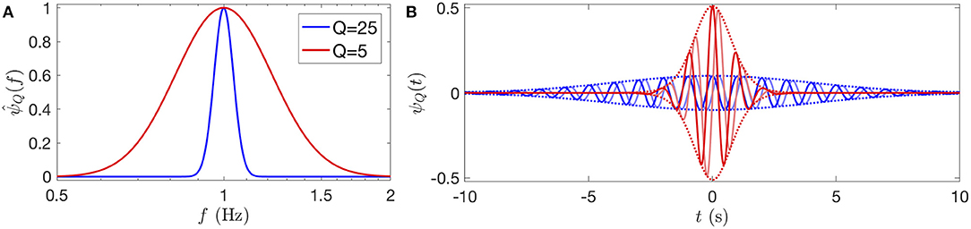
Figure 1. Grossmann log-normal wavelets of quality factor Q = 25 and 5 (in blue and red, respectively), represented in frequency in logarithmic scales (A) and in time (B), with the reference frequency f0 = 1. In (B), the real part of the wavelet is represented with a blue (respectively red) line, in quadrature, the imaginary part is a light blue (respectively light red) line, and the envelope ±|ψQ(t)| is delimited by dotted lines. The uncertainty time-frequency relation is clear here: the higher the quality factor, the more the wavelet is localized in frequency and the more it has oscillations in time. The effective number of oscillations of the wavelet are N25 ≈ 10 and N5 ≈ 2.
The CWT of the signal can be given a time-frequency interpretation when the wavelet is well-localized in the frequency domain. Indeed, while the parameter b naturally represents a time, the scale a can be associated to a frequency fp/a where fp is a characteristic frequency of the wavelet. In general, there are many ways to define this characteristic frequency [51], but for ψQ they all belong to the same family of weighted frequency average indexed by an exponent p:
The “center instantaneous frequency” f1 is obtained from the derivative of the phase of an analytic wavelet in the time domain (when this wavelet is positive in the frequency domain), the “energy frequency” f2 is used for the Heisenberg uncertainty relation, and the limit case f∞, “the peak frequency” is the frequency at the maximum of . For the Grossmann log-normal wavelet, the characteristic frequency is a function of f0 and Q: and it agrees exactly with its reference f0 frequency at its peak frequency f∞ = f0. We note also that all these frequencies fp converge to f0 for a large quality factor Q.
Notwithstanding the different frequency interpretations at low quality factor, we choose for the Grossmann wavelet the peak frequency f0 to define the frequency associated to the scale a as f = f0/a, and we denote the time-frequency representation of x(t):
Its squared modulus provides one way to define a time-varying power spectral density:
The power spectral density Sx(f) (PSD) of a stationary signal is obtained by a temporal averaging (see Supplementary File section 1):
Notice the factor |f| that appears here; it is related to the scale normalization convention chosen in the definition of the CWT. Equation (6) integrates to the power with respect to the integrator , i.e., with respect to dlogf for positive frequencies, which suggests a logarithmic (geometric) frequency sampling. This sampling is indeed natural for the CWT because the log-frequency width of its analytic wavelet is constant at all scales. Thus, we call the product Sx(f)|f| the power log-frequency density, so that the power is directly read from the area under its curve on a log-frequency axis.
Note that, contrary to more common fixed size moving temporal windows, the temporal and frequency widths of the analysing wavelet scale with the frequency [43, 44]. The square modulus of the wavelet transform XQ at point (f,t) provides a smoothed realization of the time-varying power spectral density Sx(f, t; Q). The widths of this time-frequency smoothing region are commonly estimated, similarly to f2 in Equation (3), from the variances (Δt)2 and (Δf)2 associated to the un-normalized distributions |ψ(t)|2 and . A quality factor of the wavelet can be defined as [52] and the smoothness region is well-described by the Heisenberg uncertainty relation . It means that the time and frequency resolutions cannot be both chosen arbitrarily small. In the case of the Grossmann wavelet, we can compute Δf and get up to a term of order when Q is large enough, which confirms the interpretation of its parameter. We cannot, however, get an expression for Δt. Instead, we find numerically that the effective number of oscillations at full-amplitude of ψQ(t) is very close to . For this reason, we define an effective wavelet duration , and associate to it an effective log-frequency width, very close to the full width at half maximum (FWHM) of the wavelet: . The equality fδt·δlogf = 1 is a practical variant of the Heisenberg uncertainty relation for ψQ, and it defines a time-frequency atom. This atom is interesting for sampling XQ(f, t) in a given time-frequency domain Ω, because it gives an indication of the minimum sampling points density in the time and log-frequency directions (more than one per atom).
We illustrate the time-frequency representation XQ(f, t) on a pedagogical signal x(t) = s(t)+ξ(t) in Figure 2. The signal represented in Figure 2A is the sum of a deterministic oscillation s(t) of increasing frequency (a chirp) and decreasing amplitude, and of a pink noise ξ(t) of lower amplitude [the “1/f” noise, in reference to the behavior of its power spectral density Sξ(f)]. Since is a complex value, it is represented by the amplitude A (or its square) and the phase ϕ. The factor 2 can be computed from a simple harmonic signal Acos(2πf0t) for which the modulus of the CWT is , i.e., at most for f = f0.
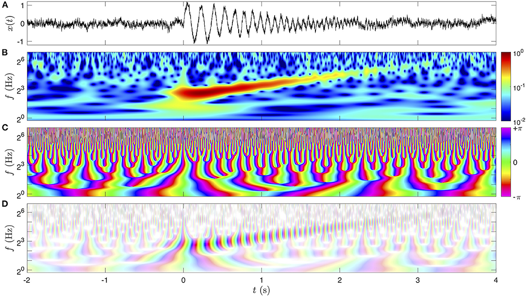
Figure 2. Graphical representations of the CWT on a pedagogical signal x(t). The signal x(t) is represented in (A), and its CWT (Equation 4) of quality factor Q = 5 is computed. The amplitude is color-coded in a logarithmic scale in (B), and the phase with the chromatic circle in (C). Note that we represented twice the amplitude of the CWT in (B) so that it is directly comparable to the amplitude of the time signal (A). Both dimensions of the complex value of the CWT are combined in (D) with a two-dimensional shaded-color coding: the phase is still associated to a hue in the chromatic circle and the amplitude is coded by the saturation of the color.
The image in Figure 2B is the amplitude of the CWT, that is maximum for t>0 at the frequencies of the chirp. The amplitude of the chirp trace decreases while its frequency increases in time. With a color-coding of A(f, t) = 2|XQ(f, t)| we observe that the maximum amplitude of the chirp in Figure 2B matches closely the amplitude of the oscillation in Figure 2A. Since we code the amplitude on a logarithmic scale, the image of its square, called the scalogram, is identical. The regions of lower amplitude appear more noisy, corresponding to the pink noise ξ(t), the amplitude of which is invariant with frequency. This is a specificity of the pink noise: it has a constant power density per decade [Sξ(f)f is constant] and has a strong physiological interest since it has been proposed to describe the scale invariance of many natural stochastic signals, such as EEGs [16, 42, 53, 54]. The pink noise was generated from a MATLAB library, applying to a white Gaussian noise a filter optimized so that the noise remains Gaussian with a constant power log-frequency density Sξ(f)|f|.
The next image in Figure 2C represents the phase of XQ(f, t), i.e., the complex argument ϕ(f, t) = ℑ{logXQ(f, t)}, which is conveniently represented with the hues in the chromatic circle since the phase is a circular quantity. In this work, the phase 0 is represented in green, ±π is in magenta and the interval from −π to π follows the progression of the colors in the visible light spectrum (at the exception of the magenta, which is not in the physical spectrum since it closes the circle). The phase in time and frequency has a particular behavior. It always increases continuously and monotonously in time, at a rate that is consistent with the frequency f: . This behavior fails near singular points in time and frequency, namely phase vortices (of unit charge), for which the phase is not defined (and the amplitude vanishes). These singular points are distributed randomly with a global density of 1 per time-frequency atom, and they are repelled from high amplitude regions. These properties result in a structure of tree for the lines of constant phase, that is branching at each singular point toward higher frequencies. “Channels” made from the repulsion of the singular points out of the high amplitude region can be noticed, where the phase progression directly represents the phase of the chirp oscillation. Remark the fast progression of the phase at a high frequency f which blurs its visualization at very large time-scales compared to the period f−1.
The last image in Figure 2D combines both the amplitude and the phase of the complex value XQ(f, t) in a two-dimensional color map. This type of shaded-color coding, possible because the color space is at least two-dimensional (three-dimensional for at least 96% of human beings), could be represented in polar coordinates (in ℂ) as a chromatic disc where the phase angle is the hue and the radius (amplitude) is the saturation of the color (no defined hue/phase if no saturation/amplitude). Here the color of vanishing amplitude is set to white, the low amplitude of the noisy regions indeed appears with very faint and pastel colors, whereas the chirp has a more intense color.
This shaded-color coding is a synthetic way of representing a map of complex values at the scale of few oscillations (otherwise the colors would hardly be distinguishable). While less suited for illustrating XQ(f, t) at large scale (only the amplitude is represented as in Figure 2B), the shaded-color coding will be ideal for time-frequency coherence maps (see reference [55] for a similar use for fMRI signals).
We focus here on three types of signals; EEG, ECG, and respiration from the PSG databases. Among these, the EEG remains the most complex, because its spectral signature is a mixture of rhythms of different natures: some of them have been recognized with a physiological origin, others which are more volatile (unsteady) can be interpreted falsely from spectral decomposition [56]. The cross-correlation of these EEG “rhythms” with other physiological signals (such as the heart and respiration rates) can help discriminate artifacts from steady rhythmic sources. Our study proposes a methodology to assist this clarification. The cardiovascular system is vital for feeding and clearing the whole body organs, its failure in the brain or other neuronal tissues leads rapidly to irreversible issues, it must therefore be finely regulated to keep a correct flux and filtration of blood. The cerebral blood flow has been reported to increase during sleep, both in slow wave sleep (4–25%) and in REM sleep (25–80%) [57]. Recently, it was also shown that the brain rhythms can be placed in resonance with the HRV and respiration when modulating the respiration frequency to lower bands [58].
Wake-sleep phases (wake, REM, and NREM) have been classified in subclasses (stages) related to different patterns of brain electrical activity, we used this classification to overlay the hypnogram from a clinician annotation (Figure 3A) with the corresponding EEG, ECG, and respiration signals (Figures 3B–D). The hypnogram is a simplified representation of sleep, based on a set of criteria about the behavior of the power density of the EEG (possibly complemented by the EOG and EMG) in the time-frequency domain, roughly discretized in frequency bands (δ up to 4 Hz, θ from 4 to 8 Hz, α from 8 to 12 Hz, σ from 12 to 16 Hz, β from 16 to 20 Hz, and γ above 20 Hz) estimated from 30 s time epochs. It is an approximation that cannot account for the continuous dynamics and the micro-structures of sleep (such as sleep spindles and K-complexes). It has been shown in reference [59] that the use of a continuous time-frequency representation of an occipital EEG can simplify considerably the scoring of the sleep stages but also their reading at the global scale of sleep, while conserving the information about micro-structures.
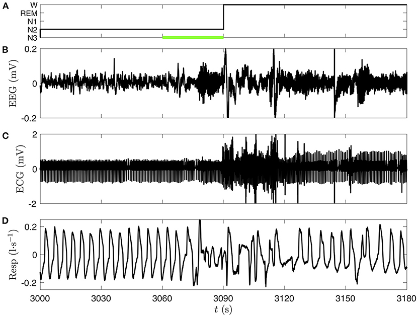
Figure 3. Comparison of three polysomnographic signals of subject slp04 selected from the database slpdb. (A) Hypnogram of the person (black line), who is shifting from NREM sleep stage 2 (N2) to wake phase (W) between 3,060 and 3,090 s. Leg movements, which were annoted by the clinician in this 30 s epoch, are represented by a green bar. (B) EEG (C3-O1) in millivolt, (C) ECG in millivolt, and (D) nasal respiration in liter per second.
We choose the EEG, ECG, and respiration signals from the same person (slp04) of the PSG database slpdb. In Figure 3, the transition from NREM stage 2 to wake phase can be noticed on the three signals. A visual inspection of the signals shows a drastic change around 3,070 s. We also note that the 30 s length epochs cannot designate with accuracy the time of this transition on the hypnogram (Figure 3A).
The scalograms (CWT-based spectrograms) corresponding to these three signals are shown in Figure 4 (same time interval). We recognize the fundamental modes of ECG (~20 = 1 Hz) and respiration signals (~2−2 = 1/4 Hz) in Figures 4D,F, and some of their harmonics (two harmonics for the ECG which are visible during the whole time interval and two harmonics for the respiration in the 3,000–3,060 time interval). The scalogram of the EEG signal is completely different, there is no clear fundamental mode. As expected, this means that the EEG is a mixture of complex dynamics spread over a large frequency range (at least up to 125 Hz and down to the instrumental cut-off visible near 1/16 Hz, illustrated in this example). On the wake stage (beyond 3,090 s) a very thin frequency band near 10 Hz corresponds to α waves, typical of the phase of wakefulness with closed eyes [59]. If we look more precisely in the N2 stage (Figure 4B) we can guess a similar band much more intermittent and less intense: it is the σ band constituted of bursts of sleep spindles. This time-frequency representation is very helpful to recognize different components; singular events are expressed as vertical structures, whereas periodic components translate in horizontal bands. Below 4 Hz we observe localized bursts (with vertical cone rather than horizontal band shape) corresponding to sharp and sudden events in the signals. The comparison in Figures 4C,E,G of the log-frequency densities estimated either directly from the squared Fourier transform (thin gray line) or from the CWT (Equation 6) (thick black line), highlights the interest of the CWT method to get a better differentiation of the peaks and of their power ratio with other non-periodic components.
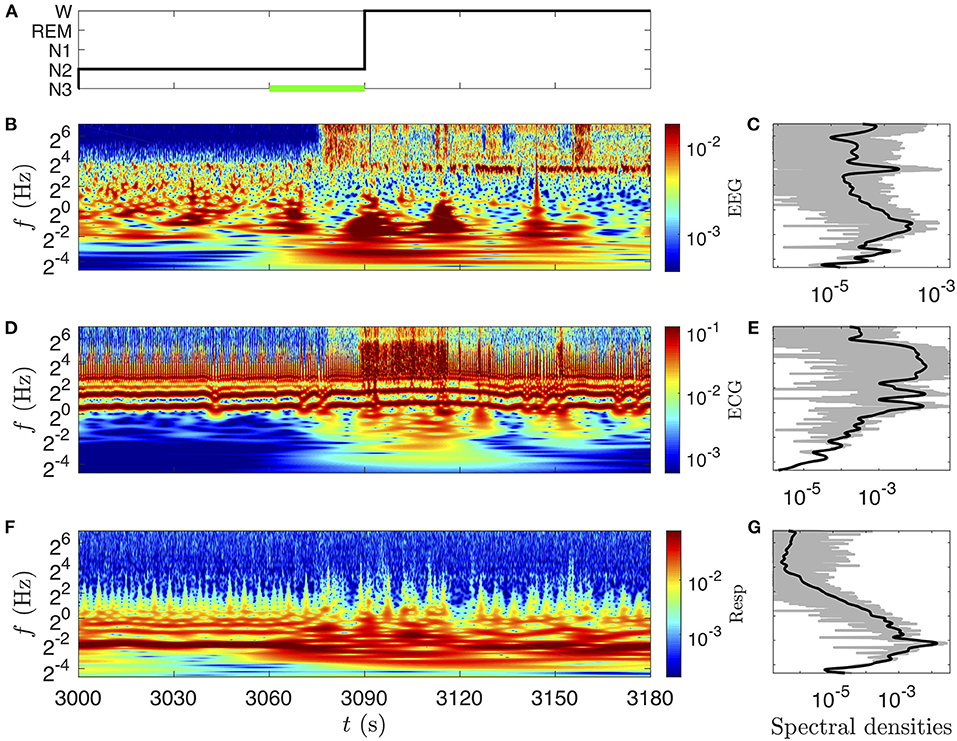
Figure 4. CWT's amplitude (twice its modulus) (B,D,F) and spectral densities (C,E,G) of the signals presented in Figure 3. (A) Hypnogram. (B) amplitude of the EEG (C3-O1) (color bar in mV) and (C) power log-frequency density (in mV2). (D) Amplitude of the ECG (color bar in mV) and (E) power log-frequency density (in mV2). (F) Amplitude of the nasal respiration signal (color bar in l·s−1) and (G) power log-frequency density [in (l·s−1)2]. The CWTs are computed with the Grossmann wavelet of quality factors Q = 10, sufficient to appreciate the frequency localization of the α EEG waves. The corresponding power log-frequency density Sx(f)|f| is estimated either directly from the squared Fourier transform (thin gray line) or from the CWT (Equation 6), (thick black line).
EEG signals are quite complex, they combine both noisy frequency bands, and aperiodic or quasiperiodic local rhythms embedded in a rather wide frequency range. The amplitude or power density changes with time within various frequency bands are straightforwardly computed from a (complex) analytic wavelet transform [60], namely the modulus |XQ(f, t)| or its square. The natural bandwidth at any frequency f is given by the width of the wavelet δlogf, which can be broadened by decreasing the quality factor Q or by mean of an integration over a larger frequency range.
Alternatively, instantaneous frequencies can be systematically extracted from the respiration and heart beat signals, yielding the respiration and heart rates. Preprocessing operations are required to obtain these signals of interest from the recordings. The extraction of the instantaneous frequency of a rhythm is generally aimed at detecting quasiperiodic oscillations (such as the ECG's peaks); it is subject to threshold choices, instabilities in certain situations and requires an homogeneous resampling. More sophisticated techniques using masking and synchrosqueezing operations (such as in [61]) are often tedious and computationally intensive. We propose here an alternative and fairly simple approach, based on the idea of slowly modulated carrier waves, that uses the CWT XQ(f, t) of a measured signal x(t).
For an ideal harmonic oscillation x(t) = Acos(2πf1t), the time-frequency representation is simply , from which we estimate the frequency as (ℑ is the imaginary part and the dot stands for a time derivative). We expect this relation to hold approximately when the frequency is slowly modulated, f1 = f1(t). This frequency estimated from the phase derivative is called an instantaneous frequency, and the time-frequency coordinate points such that f1(t) = f, called the phase ridges [51, 62] (very close to the ridge of peak amplitude). When the envelop of the oscillation is also slowly modulated, A = A(t), the CWT can be approximated by and the amplitude modulation is estimated from the real part of the logarithmic derivative: . Therefore, the logarithmic time derivative of the CWT characterizes both the frequency and the amplitude modulations (assumed to be slow).
Note that is not expected to depend heavily on f in the above idealized case. A careful selection of this frequency parameter is however essential for the estimation of the amplitude and frequency modulations in real signals, either because the signal-to-noise ratio is only high near the time-frequency ridge of the mode, or because of multiple simultaneous modes. However, we argue that these modulations can be captured in a generic way, without the help of signal-specific information, by means of a frequency average:
where w(f) is the frequency weight function. The power density of the signal at each time t is a natural choice, w(f) = |X(f, t)|2, which emphasizes the modulations of the more intense components (typically the signal) rather than the less intense ones (typically the noise). For this particular weighting, we get the simpler expression
where ẊQ(f, t) is straightforwardly computed by replacing the wavelet by in the numerical implementation of the CWT. The weight function can include a frequency band selection window, , such as a simple rectangle function on the band interval . Such band-limited frequency average will be of strong interest for screening specific EEG frequency bands and cross-correlate them with the heart and respiration rhythms. Note that reducing the band to a single frequency, χf0(f) = δ(f−f0), replaces the frequency average by an evaluation at f0: . is complex with the dimension of a rate (Hz), so that we choose to refer to it as the complex rate of a signal (given a weight function and an analytic wavelet). It can be decomposed into real and imaginary parts:
interpreted as real and instantaneous modulations of the rhythm in the signal x(t) (at the scale of the NQ ≈ Q/2.5 oscillations): is the average rate of exponential growth or decay and is the average instantaneous frequency. provides a direct and quick estimation of the HRV [63].
To test Equation (8), let us define model signals of the form A(t)z(ϕ(t)), where A(t) is the amplitude, ϕ(t) is the phase and z(t) is a periodic triangle wave. Two modulated signals will be illustrated here, x(t) with a constant amplitude and y(t) with a constant characteristic frequency:
The triangle wave z(ϕ) has the specificity of containing only harmonic frequencies of odd orders (n = 1, 3, 5, …), with an amplitude that decays as n−2 (comparable with the respiration signal).
The time-frequency analysis of these two model signals for the parameters (f0, f1, f2) = (1, 1/20, 1/60) Hz, and (a1, a2) = (0.2, 0.1), reported in Figure 5 with a quality factor Q = 5, confirms that modulations are indeed slow compared to the chosen wavelet. At higher quality factor, the modulations are not resolved entirely by the wavelet, leading to a confusion between amplitude and phase modulations. The modulated amplitude A(t) is precisely estimated by
up to an integration constant A0 (set by hand in Figures 5A,B, black lines), and the characteristic frequency is slightly overestimated by (Figures 5E,F). This separation between the average instantaneous and fundamental frequencies is due to the harmonic modes in the frequency average (Equation 8), and it increases with their weight (i.e., with the non-linearity of the oscillation). The bias is +3.6% here and it could be predicted from the oscillation's spectrum: for the triangle wave. Yet, its correction would not improve a correlation or coherence analysis since the signal will be standardized (centered and reduced). Around the ideal modulations given in Equations (10) and (11), small and fast periodic oscillations at the fundamental frequency of the rhythm can also be noticed in both types of rate signal. This non-linear effect finds its origin in pulses in the CWT (Figures 5C,D), caused by high harmonic frequencies that are not resolved by the wavelet (as soon as their harmonic order exceeds the number of wavelet oscillations NQ ≈ Q/2.5).
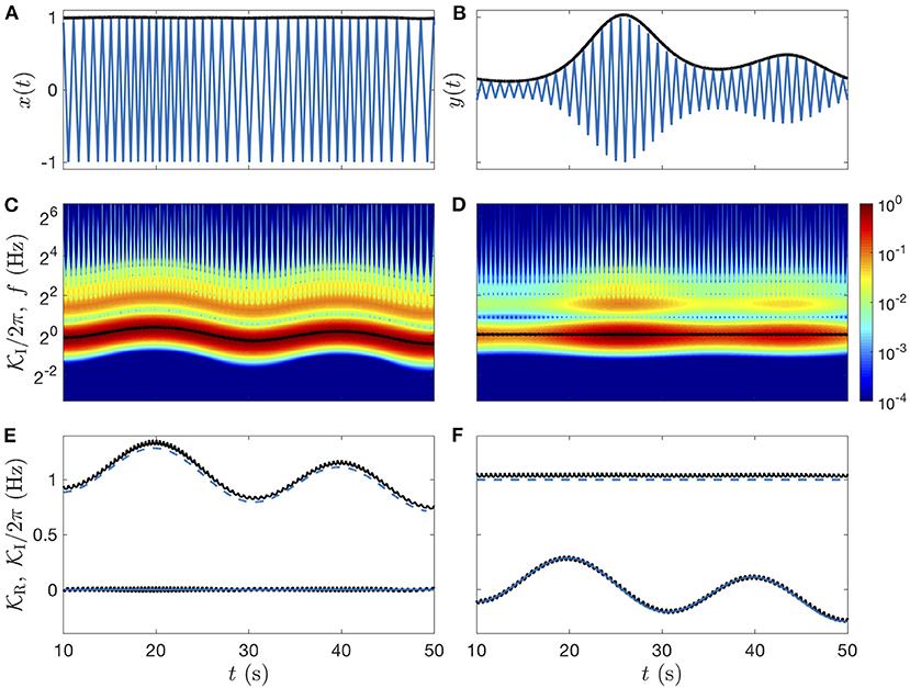
Figure 5. Idealized modulated signals: triangle waves. (A) Signal x(t) of modulated frequency and constant amplitude. (B) Signal y(t) of modulated amplitude and constant frequency. In (A,B) the amplitude modulation (estimated from Equation 12) is plotted in black lines. (C,D) Color-coded illustration of the amplitudes of the signal CWTs (twice the modulus), with their estimated frequency modulation (black lines). (E,F) Real and imaginary parts of the complex rates (Equation 8): and in black lines, are compared to the ideal values of the instantaneous frequency (blue dashed line centered to 1 Hz) and exponential rate (blue line centered to 0 Hz), see definitions in Equations (10) and (11). The Grossmann wavelet of quality factor Q = 5 is used for the CWTs and for the rates computations.
When the model signal has a much stronger non-linearity (see Supplementary Figure 2), the deviations from the ideal modulations are so important that the rate signals can not be compared directly to the true modulated amplitude and frequency. More concerning, this fast oscillation could dominate the correlation analysis of the estimated modulations, if its amplitude exceeds that ones of the true modulations.
That is precisely where the coherence analysis is helpful, since it can easily discriminate these artifacts of well-defined frequency. Amazingly, from our computations on model and real physiological signals, we have reached the conclusion that these periodic perturbations are even beneficial since they enrich the complex rate with a repetition of the carrier wave. No such oscillations are included in the usual rate estimation methods (that use lower sampling frequency).
Compared to peak extraction and re-sampling methods, common for the study of the respiration and heart rates variability, the method presented here requires no signal-specific adjustment, other than a possible frequency band selection. It also provides for free the amplitude variability (instantaneous exponential rate) in addition to the average instantaneous frequency.
The extraction of the rhythm modulations is required in order to explore their correlations beyond (lower than) their natural frequency bandwidths. These modulations are given by the complex rate (Equation 8). For illustration, we apply this method to the EEG, ECG, and respiration signals of subject slp04 from the database slpdb (see Figures 6, 7).
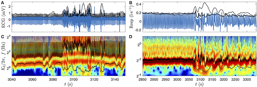
Figure 6. Illustration of the complex rate of the ECG (A,C) and of the respiration signals (B,D), from subject slp04 of slpdb near the transition from deep sleep stage to wake phase represented in Figures 4, 5. In (A,B), the physiological recording is plotted with a blue line, the amplitude estimated using (Equation 12) is the black line, and the alternative estimated amplitude is the black dotted line (see details below). (C,D) Color-coded amplitude of the signals CWT, with their frequency modulations estimated as the imaginary parts of the complex rates (Equation 8) (black lines), and the alternative estimations (black dotted line). In each panel, the alternative estimation (black dotted line) aims at reducing the non-linearity-induced oscillations (see text and Supplementary Figure 2). The Grossmann wavelet of quality factor Q = 5 is used for the CWTs. The frequency ranges shown in (C,D) are the ones used for the complex rates computation.
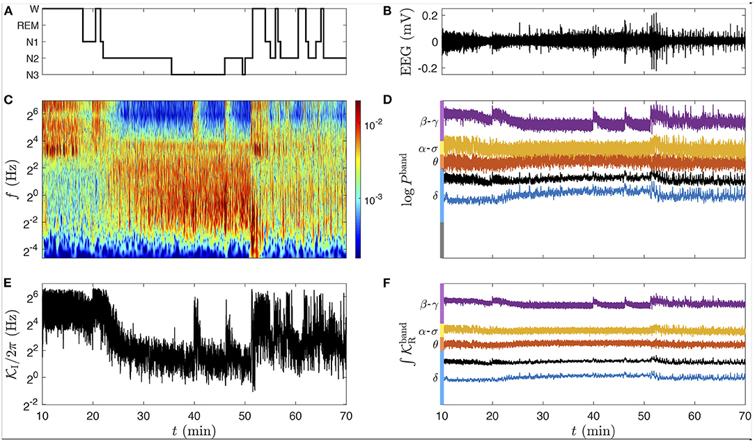
Figure 7. Modulation analysis extended to the EEG. (A) Hypnogram of the subject slp04 of slpdb during a sleep cycle: the subject falls asleep around 20 min and wakes up around 50 min. (B) EEG signal (C3-O1) in black line. (C) Color-coded amplitude of the EEG signal CWT (twice the modulus) during the selected time interval, computed with a quality factor Q = 5. The color bar gives the amplitude in millivolt. (D) Natural logarithm of the EEG band powers defined in the text and in Equation (13): Pδ in blue, Pθ in red, Pα-σ in orange, Pβ-γ in purple. The black line is the power integrated on the full frequency range (from 0.04 to 125 Hz), PEEG. (E) Average instantaneous frequency on the full frequency range. (F) Average rate of exponential growth computed in the same frequency bands as in (D). In (D,F), the central value of each signal has been aligned to the position in (C,E) of the middle frequency of its band. These signals have no dimension and are scaled in the same way.
The previous computation of from model signals (Figure 5 and Supplementary Figure 2) is reproduced easily for the respiration rhythm, yielding two additional respiration fluctuation signals and , compared in Figures 6B,D to the original respiration signal and its CWT. Extracting from an ECG perturbed by its strongly non-linear nature (Figure 7A). This non-linearity takes the form of sharp pulses of high amplitude simultaneous to the ECG pulses.
For the sake of pedagogy, a quick attempt of attenuating of this non-linear effect is proposed in Figures 6A–D (black dotted lines), using an alternative weight function (in Equation 7) to damp the high frequencies. Although the resulting average instantaneous frequencies are closer to the fundamental mode during the deep sleep stage, they are markedly shifted by low frequency perturbations, favored by the average. This is especially the case for the ECG signal when the person wakes up (Figure 6C, after 3,090 s). This alternative computation of the complex rate has the additional side effect of contaminating the modulated amplitude estimation by the opposite of the frequency modulation (as observed for the model signal in Supplementary Figure 2).
The fast oscillations in and (black lines in Figures 6A,C), are produced by the high harmonic frequencies that are not resolved by the wavelet. Those which are resolved are continuous harmonic lines that follow the modulations of the fundamental mode. They all contribute to the final complex rate proportionally to their spectral power. In the following, we will prefer this original weight function for computing the complex rate (Figure 6, black lines) to the damped version (black dotted lines) that lacks all fine details. Although these new physiological fluctuation rate signals do not compare directly to the idealized cardiac and respiration rates, their spectral richness capture all the modulations that are resolved by the wavelet in the considered frequency range (plus the carrier wave).
For the EEG, we select a longer time interval for which the subject falls asleep (around 20 min) and wakes up (around 50 min), see the hypnogram in Figure 7A. These transitions are well observable in Figure 7C from the changes of high and low frequency contents of the scalogram at these times, as in the average instantaneous frequency (Figure 8E), summarizing this behavior as the hypnogram in a suprisingly close way. Notice that we can access much more information from the CWT than from the hypnogram, such as micro-states of arousal during sleep at 40 and 46 min, yielding transient high amplitudes at the high frequencies. A conventional way to deal with the complexity of an EEG signal x is to divide it into band-limited power signals, computed straightforwardly from its CWT (Equation 5) as:
While the conventional frequency bands (δ, θ, α, σ, β, γ) are quite even in a linear frequency scale (with a width of about 4 Hz), this is not the case on a logarithmic frequency scale. For this reason, we slightly adapt the bands in this study as follows: the δ band from 0.25 to 4 Hz, θ from 4 to 8 Hz, α−σ band from 8 to 16 Hz, and the β−γ band above 16 Hz (up to 125 Hz, the Nyquist frequency limit), see Figure 7D. Since the real part of the complex rate computed in each band (Figure 7F) is used to estimate the log-amplitude in the band once integrated, we expect that describes the same modulation as the power signal (a squared amplitude) in the same band. As we can see in Figures 7D,F, and logPband are indeed indistinguishable (except for the factor 2 due to the square in Equation 13). Therefore, both kinds of signal can be used interchangeably to study the modulation of the amplitude in the EEG bands. The imaginary part of the complex rate in each band, not used in the following and hence omitted in Figure 7, could nonetheless be useful to distinguish α waves from sleep spindles in our custom α−σ band.
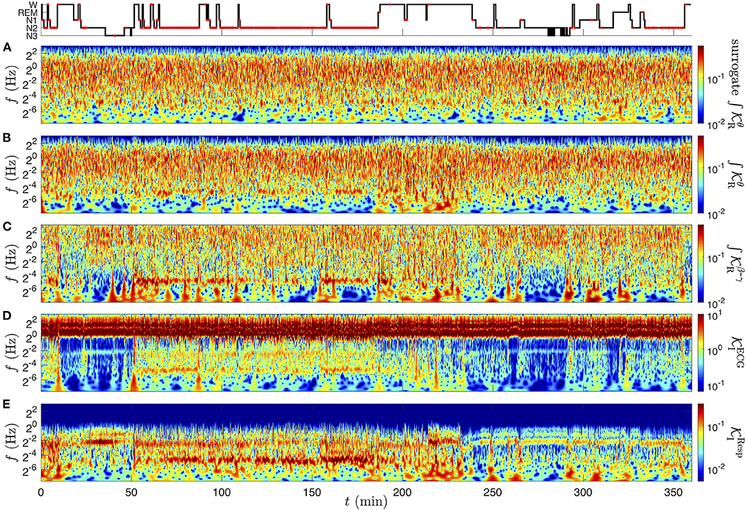
Figure 8. CWT of the physiological rate signals of subject slp04 from the database slpdb, computed as the real and imaginary parts of Equation (8). (A) Surrogate signal of (B) , the amplitude modulation in the θ band, (C) amplitude modulation in the β−γ band , (D) frequency modulation in the ECG , (E) frequency modulation in the respiration signal . The color codes for the amplitude (twice the modulus) of the CWTs, computed with the Grossmann wavelet of quality factor Q = 5. The amplitude has the unit of the signal: no dimension in (A–C), in radian per second in (D,E). At the top row, the hypnogram is marked with red dots corresponding to annotated events of obstructive apnea with arousal.
The complex rates are computed for the full overnight records of subject slp04. In particular, we discuss the modulations of the cardiac frequency, respiratory frequency, and EEG log-amplitude in the δ and β−γ bands, captured, respectively by the rate signals , , and (from Equations 8 and 9). The contributions from multiple scales, superimposed in these modulation estimators, are revealed by their CWT.
The wavelet transform is performed on two distinct levels to obtain this time-frequency rates coherence: a first CWT of each recording is required to compute its complex rate, and a second CWT is applied on the real and imaginary parts of this new complex signal. Even though the choices of the parameters could be distinct in these two rounds of CWT, we use as previously the Grossmann wavelet ψQ of quality factor Q = 5, which seems again a good compromise between a precise time localization and a sufficient frequency resolution. This fixes the wavelet widths to oscillations and (1.65 being the least distinguishable frequency ratio). The amplitudes of these CWTs are represented in Figures 8B–E. In addition, we construct a the phase-randomized surrogate of , shown in Figure 9A for Figure 8A for comparison.
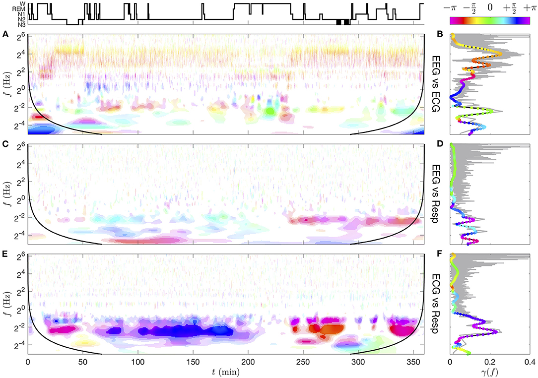
Figure 9. Time-frequency coherence γxy(f, t; Q, n) (A,C,E) and spectral coherence γxy(f) (B,D,F) computed from pairs of CWTs (see Supplementary Figure 5) for subject slp04 from the database slpdb. (A,B) EEG vs. ECG, (C,D) EEG vs. respiration signal, (E,F) ECG vs. respiration signal. The ranges of coherence moduli |γxy| for the color saturation coding are delimited by the lower thresholds γ(10−1) ≈ 0.21, γ(10−3) ≈ 0.36, 0.5, 0.7. The wavelet and smoothing kernel parameters are Q = 5 and n = 50. For each coherence image, a black line materializes a distance nδt from the initial and final times, beyond which border effects are possible. The spectral coherence γxy(f) (right column) computed from Fourier transforms (thin gray line for its modulus) is compared to the one computed from CWTs (black line for its modulus and colored dots for its phase). See text for details.
At this stage of the analysis, (Figure 8B) is hardly distinguishable from its surrogate signal (Figure 9A); they both exhibit a quite homogeneous distribution of the modulation's amplitude in the time-frequency plane (especially for the surrogate). The amplitude Figure 9B vanishes when approaching the upper frequency 8 Hz of the θ band selected for the for the θ-EEG rate computation. As observed in Figure 6, the most intense oscillations in (Figure 8D) are localized at the cardiac frequency (and its harmonics): this is the carrier frequency of the cardiac modulations in the strongly non-linear ECG signal. The information about the HRV is nonetheless present at lower frequencies: a mode of varying amplitude at 0.2 Hz confirms the known fact that the heart rate is modulated by the respiration frequency. We note that the respiration modulation intensifies, becomes unsteady and extends toward low modulation frequencies in the time interval between 50 and 180 min (NREM sleep stage 2). Apart from the respiration mode due to the non-linear carrier wave frequency, (Figure 8E) exhibits in this time-frequency region an intense mode at about 0.035 Hz. The subject slp04 is severely affected by sleep apnea, and this time interval corresponds to an uninterrupted sequence of such events (“obstructive apnea with arousal” are marked with red dots in the hypnogram). The presence of a clear mode at ~0.035 Hz means that the corresponding apneic events occur with a quite regular period: approximately every 30 s. For this reason, we refer to this phenomenon as the “apneic rhythm”. So far, we can anticipate that this apneic rhythm causes correlations between the rate signals, since it is noticeable in all rates (Figures 8B–E).
The time-frequency coherence can be viewed as a generalization of both Pearson correlation and traditional (spectral) coherence and has the advantage to preserve both temporal and spectral components of the compared signals. A rigorous definition of these quantities can be found in Supplementary Section 1. A time-frequency coherence appears to be more appropriate for the correlation analysis of single trial, non-stationary, non-linear, and/or multiscale signals produced by physiological rhythms.
This time-frequency coherence is extended from the non-stationary cross-spectrum (Equation S8), replacing the non-stationary cross Sxy(f, t) and auto-spectra Sx(f, t) and Sy(f, t) of the two signals x and y by their CWTs, XQ(f, t) and YQ(f, t):
This equation computes averages over multiple realizations of the signals, which is not applicable in general to physiological signals, apart from rather rare cases [64]. Even though the wavelet transform already performs a smoothing in both time and frequency, this averaging is of fundamental importance since it defines a finite size box over which the spectral and temporal coherence is evaluated. This quest for a correct coherence evaluation emerged from the sixties with the introduction of spectral methods in neurology [65, 66] and led to an abundant literature. We will only mention here two lines of researches which are closely related to our time-frequency approach, namely (i) single and multi-taper methods [59, 67–70] and their application to time-frequency coherence [32, 71–74] and (ii) wavelet-based coherence [55, 75–81].
Given that the wavelet effectively performs a smoothing in both time and frequency, we will use the quality factor Q for spectral smoothing and introduce another kernel (see Supplementary Section 2) with a larger size than the effective wavelet duration δt, defined in section 3.2. The width of this kernel determines both the temporal resolution of the coherence analysis and the level of spurious coherence (expected background noise of the estimator). The statistical distribution of this spurious coherence is essential to the evaluation of the coherence (see Supplementary Section 2 and Supplementary Figure 1).
The temporal smoothing of a time-frequency representation S(f, t) is performed by convolution with a positive kernel χ:
The normalized kernel is adapted to the time resolution of the CWT; note its similarity with the wavelet in Equation (1). It leads to the following estimators of the time-frequency power densities and coherence with respect to the kernel χ:
Remarkably, the temporal smoothing in Equation (15) preserves an homogeneous level of spurious coherence in the time-frequency plane (see Supplementary Section 2), while a smoothing kernel of constant duration at all frequencies implies a much greater spurious coherence at low frequencies than at higher ones as described in Torrence and Compo [77] and Gurley et al. [78].
More explicitly, we use a Gaussian time-smoothing kernel χn with a temporal spread of n times the width of the Grossmann wavelet:
for which the root mean square of the spurious coherence |γsp| is found to be very close to . The significance of the estimator is given by the distribution of the squared spurious coherence, simulated by two independent jointly stationary Gaussian noises. This spurious coherence follows a beta distribution with a single parameter β = β(Q, n), which turns out to be practically independent of Q and very close to n (when >10): β ≈ n. A simple expression for the p-value of any squared coherence level is obtained from the beta distribution:
As proposed in the context of a multi-wavelet estimator [75], it provides the threshold coherence value above which exceeds a p-level of significance. See Supplementary Section 2 and Supplementary Figure 1 for more details. As a consequence, the higher the value of n ≈ β, the more significantly we can distinguish low coherence values from the background (spurious), but the lower the time resolution. Equation (18) serves to calibrate the phase-amplitude shaded-color coding of the complex-valued map shown in Figure 2D, and thus build a synthetic visualization of the significant time-frequency coherence. The computed significance levels are then assessed from the coherence map obtained from a phase-randomized surrogate. It is worth mentioning here that well-constructed surrogates can also serve to estimate the significance directly, see for instance reference [82].
The physiological interpretation of the time-frequency coherence highly depends on the choice of the compared signals. The time-frequency coherence computed directly from the CWTs of the original records includes all the components from physiological and instrumental sources. It provides a way to locate the oscillations that are jointly collected by both measuring apparatus, regardless of their intensity in each recording. Regions of significant coherence may also indicate cross-talks between the sensors (which are preferably minimized for an optimal specificity of each measure).
We compute the CWT of the EEG, ECG, and respiration signals of subject slp04 from database slpdb with a quality factor Q = 5 (see Supplementary Figure 5). The time-frequency coherence, computed from pairs of signal CWTs with the Gaussian kernel of parameter n = 50, is represented in Figure 9. See also Supplementary Section 5 and Supplementary Figure 8 for another detailed example of coherence computation between 2 EEGs. In the panels of Figures 9B,D,F, we also compare the spectral coherence γxy(f) (Equation 8), computed from “Fourier” spectral densities (first method) and from CWTs (second method). The spectral densities are estimated in the first method from cross and squared Fourier transforms computed in 1 min windows with 30 s overlap and averaged (Welch's method), whereas in the second method, cross and squared CWTs are averaged over all times.
The most coherent region (|γxy|>0.7) lies around 0.2 Hz between the ECG and the respiratory signal (Figures 9E,F) which corresponds to repeated apneic episodes for this subject. This imprint of respiration on the ECG signal around 0.2 Hz is reminiscent of the complex interaction between autonomic system, mechanical and other factors on the excitable cells located in the sinoatrial node (respiratory sinus-arrhythmia RSA [83]). The shaded-color representation of Figure 9E shows that the phase of the coherence gets closer to π/2 (phase quadrature) during the longer NREM sleep stage 2 (N2) (typically between 100 and 180 min, in the first half of night), whereas it is in phase opposition (π or −π) when the N2 sleep stages are shorter. This heart-respiratory coordination vanishes in the wake or REM phases. Interestingly, this coordination is more visible in the EEG-respiratory pair coherence in Figure 9C in the second part of the night, with a narrower band of coherence around 0.2 Hz, and again in phase opposition.
Cardiac pulses that appear in the EEG yield another significant coherence (up to |γxy|~0.5) (Figure 9A). The high cardiac harmonic frequencies are particularly coherent with the EEG oscillations above the δ band, with a phase relation to the frequency which follows the linear trend ϕEEG−ϕECG = ±π+2πτf, where τ ≈ 14 ms. This means that the cardiac pulses in the EEG seem to appear slightly early compared to the ones in the ECG. This phenomenon is related to the one of heart-beat evoked response/potential [84].
Finally, we notice in Figure 9C two interesting features, (i) the imprint of respiration on ECG appears also in the EEG-respiration pair coherence but is more visible in the last part of the night, and it also gives a phase opposition of these two signals, (ii) another coherent mode (|γxy|~0.5) in phase opposition (magenta) between the EEG and the respiration signal appears in the very low frequency range (~0.035 Hz). An intermittent mode at 0.035 Hz is indeed noticeable in the CWT of the respiration signal (Supplementary Figure 5C), sign of a periodic loss and recovery of the lung capacity at every apneic cycle (about six respiration cycles). Such a mode can hardly be observed directly from the CWT of the EEG because of its damped amplitude at such a low frequency. In spite of this instrumental attenuation of slower oscillations, the coherence normalization compensates the loss of EEG power as long as the very weak oscillations are resolved in the signal. A close inspection of the EEG CWT (Supplementary Figure 5A) uncovers bursts (vertical singularities) about every 30 s across higher frequencies, the low frequency roots of which could produce such weak but regular oscillations at 0.035 Hz. The phase opposition with the respiration signal means that the EEG bursts occur precisely when the lung capacity is at its lowest level. The study of the very low frequency band, complicated in raw signals by their instrumental high-pass filtering, is however unleashed in modulation signals, which can oscillate arbitrarily slowly (no low frequency decay in Figure 8).
We extract first the modulations of the respiratory and cardiac frequencies and of the EEG bands with a wavelet time-frequency decomposition described in section 3.5, and we compute the cross and auto power spectral density from their wavelet transforms and the coherence from them. We use the Gaussian time-smoothing kernel χn (Equation 17) with a duration of n = 10 wavelets, giving a time-localization of 10δt ≈ 20/f, sufficient to identify the respiration rate at a resolution of 1 or 2 min and to resolve the variability of the apneic rhythm. However, the spurious coherence at a 90% level of significance (p <10−1) associated to this quite local estimator is as high as γ(10−1) ≈ 0.46 (see Equation 18): this time-frequency coherence analysis is therefore limited to rather strong correlations. The resulting time-frequency coherence of different pairs of modulation signals for the subject slp04 are represented in Figure 10.
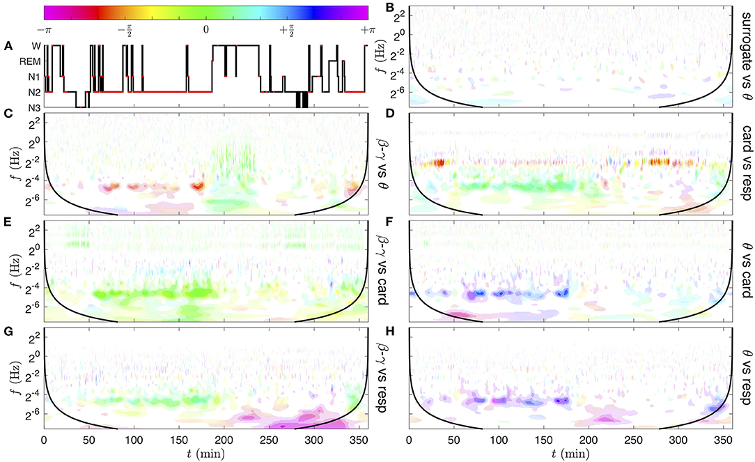
Figure 10. Time-frequency coherence analysis of the physiological rate signals pairs, obtained from their CWTs represented in Figure 8. In the following, the coherence of signal x vs. signal y corresponds to the quantity γxy(f, t; Q, n), the EEG band signals are the log-amplitude modulations estimated as , and the cardiac and respiratory rates are the frequency modulations estimated from the ECG and respiration signals as . (A) Hypnogram; the red dots corresponds to annotated events of obstructive apnea with arousal. (B) Band θ surrogate (phase-randomized signal) vs. θ. This control coherence illustrates the level of significance of the spurious coherence. (C) β−γ vs. θ band, (D) cardiac vs. respiratory rate, (E) β−γ band vs. cardiac rate, (F) θ band vs. cardiac rate. (G) β−γ band vs. respiratory rate. (H) θ band vs. respiratory rate. The ranges of coherence moduli |γxy| for the color saturation coding are delimited by the lower thresholds γ(10−1) ≈ 0.46, γ(10−3) ≈ 0.71, 0.8, 0.9. The quality factor of the Grossmann wavelet is Q = 5 and the Gaussian time-smoothing parameter is n = 10. For each coherence image, a black line materializes a distance nδt from the initial and final times, beyond which border effects are possible.
The most striking observation in Figure 10 is an intermittent but strong coherence in the frequency band near 0.035 Hz, between 50 and 180 min, in all pairs of physiological rate signals (Figures 10C–H) (which can extend to 200 min, and is also visible around 340 min). By comparing the time intervals in which this apneic rhythm appears with the annotations of the hypnogram (Figure 10A), we notice that it only occurs during the NREM sleep stage 2 (N2) and that the coherence decreases or disappears when the person wakes up (W). coherence decreases or disappears when the person wakes up (W). The different colors of this region indicate different phase shifts between rates. For instance, in Figure 10C, the EEG β−γ band is to radians delayed (late) compared to the EEG θ band. This means that not only these two EEG frequency bands behave coherently, but also that they are quite in phase opposition; while the EEG signal in the θ band reaches its maximum, the EEG signal in the β−γ band increases progressively from its lowest value. In Figure 10D, the small phase shift between and indicates that the decreases and increases of the cardiac and respiratory rhythms occur quasi in-phase at each cycle of apnea (or the cardio-apneic rate variation slightly precedes the respiratory one). The light green color of the apneic coherent region in the next panels (Figures 10E–H) indicates that the cardiac and respiratory modulations evolve nearly in phase with the EEG β−γ band, while it is rather in phase opposition with the EEG θ band (purple blue color).
We can also observe in Figure 10G a region of strong coherence (|γ|~0.8−0.9) in phase opposition (magenta), from 250 to 340 min at very low frequencies (below 2−6~0.02 Hz, i.e., at the scale of a few minutes). As can be checked in Supplementary Figures 5A,C, this region corresponds to isolated events of apnea (at times 250, 265, 292, 303, 306, 324 min), with relatively quick drops and restoration of the respiration frequency and simultaneous rise and disappearance of β−γ amplitude in the EEG. These kinds of micro wake states may constitute a different recovery mechanism, slower than the apneic rhythm around 0.035 Hz.
Other regions of significant coherence can be observed. In Figure 10D, the modulation of the cardiac rate by the respiration in the frequency range 0.1–0.4 Hz is also observed in some time intervals (from 30 to 40 min and from 270 to 320 min). Amazingly, the strong coherence which was computed from the CWTs of the raw signals (Figure 9E) has quite disappeared, in particular during the sleep apnea episodes. Comparatively, the coordination of the apneic rhythm has a much stronger echo in the EEG signals.
In Figure 10E, in-phase coherent lines at the cardiac fundamental and harmonic frequencies highlight the presence of cardiac impulses in the β−γ band of the EEG (also visible but less significant in the θ band). Interestingly, a slight coherence of phase shift , at the respiratory frequency from 100 to 150 min, also appears between the cardiac rate and the β−γ amplitude.
This evidence questions the relation of the apneic rhythm to a dysfunction of the autonomic regulation of cardio-pulmonary coupling during sleep apnea [83, 85]. The fact that the coherence phase changes in subject slp04 when comparing different EEG frequency bands [β−γ and θ illustrated in Figures 10E–H] could suggest a different implication of sub-groups of neurons in this regulation. Brain inter-band EEG correlation patterns have recently been demonstrated in different sleep stages [86], by the computation of a Pearson correlation coefficient ρxy from pairs of frequency bands. This distinguishes well in-phase fluctuations from those in phase opposition, however both positive or negative phase quadrature (e.g., due to a differential relation) lead to a vanishing correlation. Extending the Pearson correlation ρxy to a complex correlation coefficient (or global coherence) (Equation S6), that takes values in the unit disk, could restore a whole 2π interval of phase-shift values. The observation of heterogeneous EEG inter-band coherence in Figure 10 and Supplementary Figure 7 further suggests the importance of introducing the spectral localization (i.e., the coherence γxy) for contributions of slow and fast modulations [87]. Finally, in (Figure 10C) a wide domain of in-phase coherence (green) appears between the θ and β−γ bands when the person is awake (from 190 to 240 min), while this type of correlation damps out during sleep (apart from the apneic rhythm). An explanation could be found in the singular events crossing the full frequency range, possibly related to motions of the waked person. The complete EEG inter-band coherence analysis (for all EEG band pairs) is presented in the Supplementary Figure 7.
The richness of the proposed time-frequency method offers more analytic perspectives than those tested in here. In the case of EEGs for instance, the modulation of the amplitude (or power) in each band could be compared to the EEG itself; such a choice of input signals for a coherence analysis could help understand the relations between the phase of slow waves (e.g., δ) and the modulations of faster ones (e.g., sleep spindles).
This thorough coherence analysis of the subject slp04 points out the interest of the method proposed in this work, generalizing it to the shhs2 polysomnography database in next section 5, brings a statistical confirmation of its validity, as compared to other analysis of the HRV published in the last two decades [88–90].
Finally, we complete this study with a statistically robust analysis of a large selection of subjects from the shhs2 database, distributed in five groups defined by their type of sleep apnea (see section 2.4).
Before selection, an individual analysis of the rates coherence (Figure 10) is performed from all the subjects of the shhs2 database. The statistics is performed in each group by averaging in time, over the selected and cumulated intervals, the time-frequency squared coherence . This reduces the huge amount of generated individual data to the typical intensity of synchrony defined as the squared coherence between the physiological rate signals, across frequencies and apnea groups. Note that the square is essential here to focus on the average instantaneous coherence strength. It prevents the sleep stages and inter-personal variabilities of the coherence phase (complex argument) from reducing the global mean intensity, as would be the case when estimating the (stationary) spectral coherence. The distribution of the phase can be studied separately.
The coherence profiles, resulting from the conditional averaging of over the full cumulated times of apnea in each group, are compared in Figure 11 for three pairs of modulation signals from the heart, breathing and brain activity. The total duration of these averaging intervals (for each sub-group H, O, and C) is very long compared to the width of the (time) smoothing kernel (of characteristic duration s for our estimate), which makes these profiles very robust. They can further be compared to the expected spurious coherence level (gray thick dashed line in Figure 11) fixed by the time smoothing parameter n = 10.
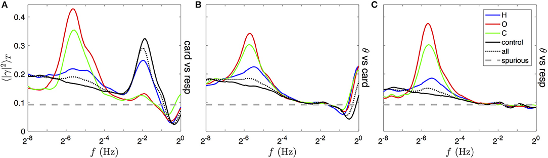
Figure 11. Comparison of typical squared coherence profiles for different sleep apneas and from different rate signals pairs, obtained from the full database shhs2. In each panel, colored lines are obtained by averaging the squared modulus of the time-frequency coherence, , over the time duration of apneic events in distinct groups: 87 subjects strongly affected by hypopnea (blue lines), 153 by OSA (red lines) and 189 by CSA (green line). See text for details of the selection. The black line is the average over the full sleep duration of a control group very mildly affected by any type of apnea, the black dotted line is the unconditional average over the full sleep duration of all 2,650 subjects in the database, and the gray thick dashed line traces the expected level of spurious coherence. These profiles are mean squared coherences between (A) the cardiac vs. respiratory rate, (B) the θ band vs. the respiratory rate and (C) the θ band vs. the cardiac rate modulation signals, as shown for a single subject in Figures 10D,F,H before squaring and time averaging.
CSA and OSA are associated with the rise of a peak of coherence between all pairs of rate signals, maximum around 0.02 Hz, on the group C and O (green and red lines in all panels of Figure 11). This mode is much less prominent in the group H (blue line) and absent from the control group (black line); instead the baseline of coherence at very low frequency is enhanced. This band corresponds to the “apneic rhythm” in the breathing and heart rates and in every band of the EEG activity (only θ band, shown in Figures 11B,C). In contrast, a peak of coherence at the respiratory frequency (near 1/4 Hz) is visible in Figure 11A only, meaning that the heart rate is modulated by the breathing cycle [this is the respiratory sinus arrhythmia (RSA)]. Contrary to the slower coherent mode, this modulation is most coherent in the control and the H group, whereas it is almost incoherent in the C and O groups.
The asymmetric shape of these two coherent modes can be explained as follows: (i) the bandwidth of the Grossmann wavelet δlogf covers less than an octave (from the quality factor Q = 5), and imposes a log-normal shape and a minimum width to isolated and non-averaged coherence peaks; (ii) the variability of the frequency of both coherent modes over times and subjects in each group is likely to spread the averaged peaks on larger widths (>1 octave); (iii) before averaging, a second peak (harmonic mode) of lower coherence can be distinguished, with frequency shifted one octave higher than the fundamental one.
Furthermore, a coherent mode at the cardiac frequency (at 1 Hz and above) is visible in panel B for all group averages. It is due to the presence of cardiac pulses in the EEG (studied as the heart-beat evoked response/potential [84]). Finally, a decrease of the coherence level below the expected spurious level can be noticed between the breathing and cardiac frequencies in Figures 11A,B.
We use the PhysioNet cardiovascular signal toolbox [91] to compute the HRV signals from the ECG's RR intervals (jqrs algorithm), corrected automatically for ectopic and non-normal beats. We then compute the typical power spectral density profiles corresponding to each group as in Figure 11 as follows: (i) we obtain the CWT squared modulus (Q = 5) of the heart rate signal of each subject in shhs2, (ii) we select the subjects of each group and the time intervals with sleep apnea as previously (section 5.1), (iii) we perform the (conditional and unconditional) time averages for each subject. Figure 12A is then obtained by averaging individual spectra in each group, weighted by the duration of each individual time selection, whereas in Figure 12B the individual spectra are normalized prior to the group average (also weighted by individual duration). As a result, the profiles in (A) give mean absolute values for these HRV spectra, whereas (B) shows the mean profiles relative to the strength of the HRV (by normalizing out strong or weak individual HRV).
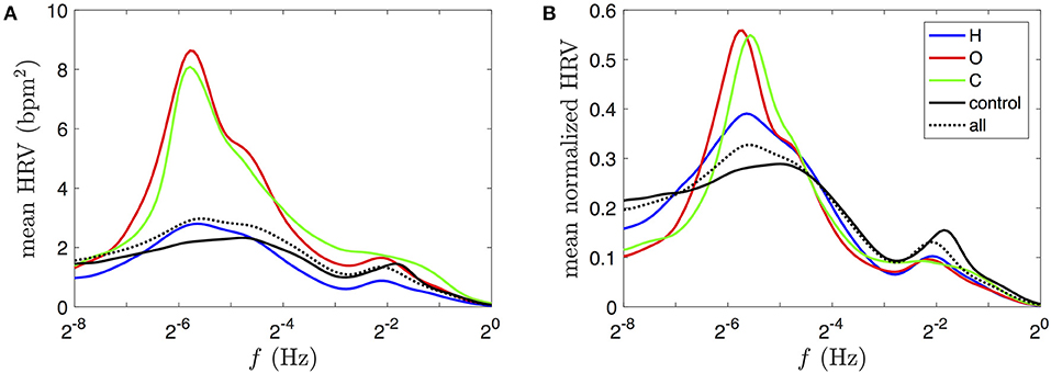
Figure 12. Comparison of typical HRV power spectral densities, obtained from the full database shhs2. (A) Power log-frequency density of the HRV signal, in bpm2, obtained by averaging its squared CWT in time (see Equation 6) over the selected time durations for the same subject groups as those used for Figure 11 (using the same color coding). (B) Time-averaged spectra, normalized for each subject prior to the group average (weighted by individual durations). The heart rate signals are estimated for each subject's ECG from the corrected RR interval.
The only difference between the data selection in Figures 11, 12 lies in an additional data exclusion of all 10-s epochs of non-physiological RR intervals (outside 0.375 to 2s during more than 15% of the duration, before correction). This mask excludes about 5–10% of the total durations in each group. The mean normalized HRV spectra in Figure 12B are nearly insensitive to this procedure compared the ones obtained without any data exclusion or with a stricter selection criterion (sqi>0.9, excluding 25–30% of the heart rate duration that does not coincide with the alternative estimation from the sqrs algorithm). These selections, supposedly affected by detection artifacts, tend to have strong amplitudes, so that their exclusion leads to a global decrease of the values of the mean HRV spectra in Figure 12A.
A first observation is the clear correspondence between rates coherence and HRV power spectra profiles, in particular we note the presence of a peak at low frequencies in Figures 11, 12, especially prominent in the case of obstructive and central sleep apneas. In the respiratory frequency band, however, differences between the groups are much harder to grasp from the HRV power spectra: the control group seems to have a significantly higher proportion of respiratory HRV (RSA) than the apneic groups (Figure 12B). This inversion of intensity from the low frequency to the respiratory bands between apneic and healthy subjects was much easier to discriminate in the rates coherence profiles (Figure 11A).
While these two measures both describe a certain intensity of the physiological activity in these frequency bands, their interpretation is very different. The HRV power spectra is limited to quantify the extent of the HRV amplitudes across frequencies, while the cardio-respiratory rates coherence of Figure 11A characterizes the quality of the synchrony, regardless of these amplitudes.
Based on all the above presented profiles for central and obstructive sleep apnea, we finally give our estimation of the localization of the fundamental apneic (low frequency) mode: the global maximum lies at 0.019±0.002 Hz (i.e., a period of 12–15 breathing cycles), and the widths suggests a variability of this rhythm among subjects ranging from 0.011 to 0.038 Hz (i.e., 1.8 octave).
We addressed the question of characterizing the coherence between distinct dynamics inside a physiological network. As suspected quite early (250 years for the heart rate), the variability (modulation) of these rhythms is at the core of neural regulation of organ systems, such as the cardiovascular and respiratory systems considered in this study. Analysing pair-wise interactions under the angle of a coherence analysis, we highlighted the high level of complexity of polysomnography database signals. Their non-stationarity, their nonlinearity and their wide frequency ranges are all taken into account without needing any pre-processing treatment (such as spectral whitening/detrending, or rank statistics). Moreover, this time-frequency extension of the correlation analysis is a starting point for the study of interaction network (see for instance [92]), which directly benefits from analytic expressions for the significance of the estimators, multidimensional refinements, such as multiple and partial correlations [93], as well as more recent directed versions of the coherence [25, 94]. We believe this is the natural framework to recast the questions of correlations, synchronization, delays, and the search for their stability and persistence, strengthening their physical roots.
It has been recognized since the sixties that the autonomous nervous system is undergoing profound changes during sleep [95], and that these changes can be traced in the sleep stages [96]. The autonomic nervous system regulation of the cardiovascular system changes from N1 to N3 sleep stages, the parasympathetic nervous system getting predominant at deeper sleep stages. Spectral analysis of the HRV was widely used in the last decades [8, 63, 97], and led to distinguishing three frequency bands: (i) a low frequency band (LF) (0.04–0.15 Hz), representing both sympathetic and parasympathetic (vagal) regulation, (ii) a high frequency band (HF) (0.15–0.40 Hz) where the parasympathetic regulation dominates and (iii) a very low frequency band (VLF) (below 0.04 Hz) where sleep-related respiration disorders, thermo or vasomotor regulation mechanisms could be involved [63, 98].
We proposed a novel method, namely the complex rate, to extract the instantaneous temporal variation of frequency and amplitude of rhythms directly and simultaneously from the wavelet transform of the original (raw) records, and we described how they differ from the signals extracted by other methods. From these modulation signals, we computed a time-frequency coherence based on the Grossmann wavelet and we revealed both the spectral and temporal structure of the correlation between the cardiac, respiratory rates variability, and the neural activity in distinct frequency bands. Our wavelet-based computation of the complex rate was straightforward and did not require usual preprocessing steps [98]. The manipulation of complex-valued maps, such as XQ(f, t) or γxy(f, t) was shown to be of major importance to account for the richness of the dynamics under consideration. Their high dimensionality can however discourage their full visualization which could explain the few attempts existing in the literature (the color coding is often limited to the real-valued squared modulus). For this reason, we believe that our use of a polar color-shaded coding (saturation and hue) for the modulus and the phase was also a useful achievement of this work, yielding a synthetic graphical visualization.
We first focused on a subject affected by obstructive sleep apnea to illustrate how slow rhythmic events related to apnea and recovery were ubiquitous in the modulations from all the records (EEG in all bands, ECG and respiration), pointing out the strong interaction of different organs involved in the mechanisms associated to apnea. After exploring the rich phenomenology of individual polysomnographic recordings, we repeated this analysis on all subjects of the shhs2 database and we exposed a statistical analysis of the rates squared coherence profiles for different types of sleep apnea in a large database of apneic subjects, and compared it to averaged HRV spectra.
Without any preprocessing or filtering of the data, we showed that apnea intervals were unambiguously related to an apneic modulation in the VLF frequency band of the neural, cardiac and respiratory rhythms. For severe sleep apnea, this modulation is most coherent and rhythmic, with a quite well-defined fundamental frequency localized not farther than an octave from 0.02 Hz (depending on the subject). It is also easily observable from the oxygen saturation (SpO2) recordings provided by the slpdb database, and it clearly corresponds to a peak in the HRV power spectra at the same frequency. The increase of this rate coherence and HRV power in the VLF band is concomitant with the decrease of a second coherent mode a decade higher: the well-known heart rate modulation by the breathing cycle (respiratory sinus arrhythmia (RSA) [83] in the HF band). This trade-off between the activities in the VLF and the HF bands, which is harder to grasp from the HRV power spectra, corresponds to an increased sympathetic activity and decreased vagal (parasympathetic) activity [4, 5] during sleep apnea (and hypopnea to a lesser extent).
Finally, the HRV power spectra, which can be computed from ECGs only, are therefore easier to capture and to analyse. However, they measure only the extent of the HRV amplitudes across frequencies, while the cardio-respiratory rates coherence characterizes the quality of their synchrony, regardless of the amplitude of the modulations. This can be used to capture intervals of synchronization from a pair of oscillators, also giving access to their phase shift. Cardio-respiratory synchronization is not generally recorded in rest or sleep, it has been observed during specific breathing and/or vocal exercises [99, 100].
The analytic wavelet decomposition that underlies our time-frequency method shares a deep connection with the Hilbert transform, used in other phase detection methods. For instance, at the basis of the construction of synchronization indices and coupling functions between the heart and breathing phases [101, 102], the non-linear Hilbert protophase is transformed into a genuine (linear) phase from the preliminary estimation of the noise-free oscillation shapes. In the analytic wavelet transform of a rhythmic oscillation, this genuine phase is estimated “on the fly” from the phase of the fundamental mode, while harmonic modes account for non-linearities (i.e., the mismatch between the recorded oscillations and our generic wavelet shapes). Preliminary estimations, such as correct window sizes for highly noisy and non-stationary signals can be the most difficult task. They reduce in our approach to the choice of a quality factor Q for the wavelet transform, and the size of the time-averaging kernel n in the coherence analysis. We have discussed their role in the compromises between resolutions and significance.
We showed how the time-frequency coherence can overcome the comparisons of signals of very different spectral and temporal signatures and uncover otherwise hidden or mixed correlations. In particular, the cardiac and respiration rhythms were identified in the EEGs with different intensities, overlaps which are rarely taken into account [42]. Such a cross-talk is also expected between EEGs recorded at distant locations, and their alternating coherence patterns (strong or weak, in-phase or out-of-phase, in different frequency bands), could be used to study sleep stages. This is illustrated in the Supplementary Material for two EEG signals recorded contralateraly from a subject of the shhs2 database. In spite of their expected very strong and global correlation, we observe in Supplementary Figures 8, 9 the emergence of different patterns related to the phases of sleep. The rate coherence from other EEG frequency bands have also been investigated (Supplementary Figure 7), and we have been rather amazed by the variety and richness of cross-couplings (in phase and intensity) that our rather simple method could uncover. This reinforces the complementarity of the time-frequency coherence for physiology signals investigation to other methods aiming at reconstructing phases coupling [101, 102] for characterizing sleep disorders and their organic or central nervous system origin [29, 97]. It also provides a complete and visual picture of correlations between distant zones and should help addressing new issues in Network Physiology [3, 103, 104].
The original contributions presented in the study are included in the article/Supplementary Material, further inquiries can be directed to the corresponding author/s.
AA and FA: conception and design. AG, AA, and FA: development and methodology and analysis and interpretation of data. AG and FA: writing, review, and/or revision of the manuscript. FA: administrative, technical, or material support (i.e., requiring and organizing data, constructing databases). All authors contributed to the article and approved the submitted version.
This work was supported by Agency of National Research (France)—contract: ANR-18-CE45-0012-01. The Sleep Heart Health Study (SHHS) was supported by National Heart, Lung, and Blood Institute cooperative agreements U01HL53916 (University of California, Davis), U01HL53931 (New York University), U01HL53934 (University of Minnesota), U01HL53937 and U01HL64360 (Johns Hopkins University), U01HL53938 (University of Arizona), U01HL53940 (University of Washington), U01HL53941 (Boston University), and U01HL63463 (Case Western Reserve University).
The authors declare that the research was conducted in the absence of any commercial or financial relationships that could be construed as a potential conflict of interest.
We acknowledge support from the Agence Nationale de la Recherche (ANR grant number ANR-18-CE45-0012-01). AG acknowledges support from EURLight S&T Ph.D. funding. We were indebted to J. Bitton who put the coherence on our way, to J. Taillard from SANPSY USR CNRS 3413, University of Bordeaux for insightful remarks on EEGs and sleep research, and to P. Argoul, E. Harte, S. Polizzi for fruitful discussions. PhysioNet, originally established under the auspices of the National Center for Research Resources (NCRR) of the National Institutes of Health (NIH) until 2011, now gratefully acknowledges ongoing support from the National Institute of General Medical Sciences (NIGMS) and National Institute of Biomedical Imaging and Bioengineering (NIBIB) under grant R01GM10498.
The Supplementary Material for this article can be found online at: https://www.frontiersin.org/articles/10.3389/fams.2021.624456/full#supplementary-material
1. Bashan A, Bartsch RP, Kantelhardt JW, Havlin S, Ivanov PC. Network physiology reveals relations between network topology and physiological function. Nat Commun. (2012) 3:702. doi: 10.1038/ncomms1705
2. Bartsch RP, Ivanov PC. Coexisting forms of coupling and phase-transitions in physiological networks. In: Mladenov VM, Ivanov PC, editors. Nonlinear Dynamics of Electronic Systems, Vol. 438. Cham: Springer International Publishing (2014). p. 270–87. doi: 10.1007/978-3-319-08672-9_33
3. Ivanov PC, Liu KKL, Bartsch RP. Focus on the emerging new fields of network physiology and network medicine. New J Phys. (2016) 18:100201. doi: 10.1088/1367-2630/18/10/100201
4. Moser M, Frühwirth M, Penter R, Winker R. Why life oscillates? From a topographical towards a functional chronobiology. Cancer Causes Control. (2006) 17:591–9. doi: 10.1007/s10552-006-0015-9
5. Moser M, Fruhwirth M, Kenner T. The symphony of life [chronobiological investigations]. IEEE Eng Med Biol Mag. (2008) 27:29–37. doi: 10.1109/MEMB.2007.907365
6. Tomen N, Herrmann JM, Ernst U editors. The Functional Role of Critical Dynamics in Neural Systems. Springer Series on Bio- and Neurosystems, Vol. 11. Cham: Springer International Publishing (2019). doi: 10.1007/978-3-030-20965-0
7. Saleur H, Sammis CG, Sornette D. Discrete scale invariance, complex fractal dimensions, and log-periodic fluctuations in seismicity. J Geophys Res Solid Earth. (1996) 101:17661–77. doi: 10.1029/96JB00876
8. Ivanov P, Rosenblum M, Peng CK, Mietus J, Havlin S, Stanley H, et al. Scaling and universality in heart rate variability distributions. Phys A Stat Mech Appl. (1998) 249:587–93. doi: 10.1016/S0378-4371(97)00522-0
9. Ivanov PC, Amaral LAN, Goldberger AL, Stanley HE. Stochastic feedback and the regulation of biological rhythms. Europhys Lett. (1998) 43:363–8. doi: 10.1209/epl/i1998-00366-3
10. Hu K, Ivanov PC, Chen Z, Hilton MF, Stanley H, Shea SA. Non-random fluctuations and multi-scale dynamics regulation of human activity. Phys A Stat Mech Appl. (2004) 337:307–18. doi: 10.1016/j.physa.2004.01.042
11. Ivanov PC, Chen Z, Hu K, Eugene Stanley H. Multiscale aspects of cardiac control. Phys A Stat Mech Appl. (2004) 344:685–704. doi: 10.1016/j.physa.2004.08.016
12. Bernaola-Galvan P, Ivanov PC, Nunes Amaral LA, Stanley HE. Scale invariance in the nonstationarity of human heart rate. Phys Rev Lett. (2001) 87:168105. doi: 10.1103/PhysRevLett.87.168105
13. Ivanov PC, Bunde A, Amaral LAN, Havlin S, Fritsch-Yelle J, Baevsky RM, et al. Sleep-wake differences in scaling behavior of the human heartbeat: analysis of terrestrial and long-term space flight data. Europhys Lett. (1999) 48:594–600. doi: 10.1209/epl/i1999-00525-0
14. Lo CC, Amaral LAN, Havlin S, Ivanov PC, Penzel T, Peter JH, et al. Dynamics of sleep-wake transitions during sleep. Europhys Lett. (2002) 57:625–31. doi: 10.1209/epl/i2002-00508-7
15. Lo CC, Chou T, Penzel T, Scammell TE, Strecker RE, Stanley HE, et al. Common scale-invariant patterns of sleep-wake transitions across mammalian species. Proc Natl Acad Sci USA. (2004) 101:17545–8. doi: 10.1073/pnas.0408242101
16. He BJ. Scale-free brain activity: past, present, and future. Trends Cogn Sci. (2014) 18:480–7. doi: 10.1016/j.tics.2014.04.003
17. Lombardi F, Wang JW, Zhang X, Ivanov PC. Power-law correlations and coupling of active and quiet states underlie a class of complex systems with self-organization at criticality. EPJ Web Conf . (2020) 230:00005. doi: 10.1051/epjconf/202023000005
18. Botcharova M, Farmer SF, Berthouze L. Markers of criticality in phase synchronization. Front Syst Neurosci. (2014) 8:176. doi: 10.3389/fnsys.2014.00176
19. Wilting J, Priesemann V. 25 years of criticality in neuroscience—established results, open controversies, novel concepts. Curr Opin Neurobiol. (2019) 58:105–11. doi: 10.1016/j.conb.2019.08.002
20. Zimmern V. Why brain criticality is clinically relevant: a scoping review. Front Neural Circuits. (2020) 14:54. doi: 10.3389/fncir.2020.00054
21. Wang JWJL, Lombardi F, Zhang X, Anaclet C, Ivanov PC. Non-equilibrium critical dynamics of bursts in θ and δ rhythms as fundamental characteristic of sleep and wake micro-architecture. PLoS Comput Biol. (2019) 15:e1007268. doi: 10.1371/journal.pcbi.1007268
22. Lombardi F, Gómez-Extremera M, Bernaola-Galvan P, Vetrivelan R, Saper CB, Scammell TE, et al. Critical dynamics and coupling in bursts of cortical rhythms indicate non-homeostatic mechanism for sleep-stage transitions and dual role of VLPO neurons in both sleep and wake. J Neurosci. (2020) 40:171–90. doi: 10.1523/JNEUROSCI.1278-19.2019
23. Xiong W, Faes L, Ivanov PC. Entropy measures, entropy estimators, and their performance in quantifying complex dynamics: Effects of artifacts, nonstationarity, and long-range correlations. Phys Rev E. (2017) 95:062114. doi: 10.1103/PhysRevE.95.062114
24. Faes L, Marinazzo D, Stramaglia S, Jurysta F, Porta A, Giandomenico N. Predictability decomposition detects the impairment of brain-heart dynamical networks during sleep disorders and their recovery with treatment. Philos Trans R Soc A Math Phys Eng Sci. (2016) 374:20150177. doi: 10.1098/rsta.2015.0177
25. Baccala LA, Sameshima K. Partial directed coherence: a new concept in neural structure determination. Biol Cybernet. (2001) 84:463–74. doi: 10.1007/PL00007990
26. Barnett L, Barrett AB, Seth AK. Granger causality and transfer entropy are equivalent for Gaussian variables. Phys Rev Lett. (2009) 103:238701. doi: 10.1103/PhysRevLett.103.238701
27. Chicharro D. On the spectral formulation of Granger causality. Biol Cybernet. (2011) 105:331–47. doi: 10.1007/s00422-011-0469-z
28. Faes L, Stramiglia S, Marinazzo D. On the interpretability and computational reliability of frequency-domain Granger causality. F1000Research. (2017) 6:1710. doi: 10.12688/f1000research.12694.1
29. Bartsch RP, Liu KK, Ma QD, Ivanov PC. Three independent forms of cardio-respiratory coupling: transitions across sleep stages. Comput Cardiol. (2010) 41:781–4.
30. Bartsch RP, Schumann AY, Kantelhardt JW, Penzel T, Ivanov PC. Phase transitions in physiologic coupling. Proc Natl Acad Sci USA. (2012) 109:10181–6. doi: 10.1073/pnas.1204568109
31. Carter G. Coherence and time delay estimation. Proc IEEE. (1987) 75:236–55. doi: 10.1109/PROC.1987.13723
32. Lovett EG, Ropella KM. Time-frequency coherence analysis of atrial fibrillation termination during procainamide administration. Ann Biomed Eng. (1997) 25:975–84. doi: 10.1007/BF02684133
33. Saab R, McKeown M, Myers L, Abu-Gharbieh R. A wavelet based approach for the detection of coupling in EEG signals. In: Conference Proceedings. 2nd International IEEE EMBS Conference on Neural Engineering. Arlington, VA: IEEE (2005). p. 616–20.
34. Orini M, Bailon R, Mainardi LT, Laguna P, Flandrin P. Characterization of dynamic interactions between cardiovascular signals by time-frequency coherence. IEEE Trans Biomed Eng. (2012) 59:663–73. doi: 10.1109/TBME.2011.2171959
35. Rechtschaffer A, Kales A. A Manual of Standardized Terminology, Techniques and Scoring System for Sleep Stages of Human Subjects. Bethesda, MD: National Institute of Health (1968).
36. Grigg-Damberger MM. The AASM scoring manual four years later. J Clin Sleep Med. (2012) 8:323–32. doi: 10.5664/jcsm.1928
37. Goldberger AL, Amaral LAN, Glass L, Hausdorff JM, Ivanov PC, Mark RG, et al. PhysioBank, PhysioToolkit, and PhysioNet: components of a new research resource for complex physiologic signals. Circulation. (2000) 101:E215–20. doi: 10.1161/01.CIR.101.23.e215
38. Zhang GQ, Cui L, Mueller R, Tao S, Kim M, Rueschman M, et al. The National Sleep Research Resource: towards a sleep data commons. J Am Med Inform Assoc. (2018) 25:1351–8. doi: 10.1093/jamia/ocy064
39. Quan SF, Howard BV, Iber C, Kiley JP, Nieto FJ, O'Connor GT, et al. The sleep heart health study: design, rationale and methods. Sleep. (1997) 20:1077–85.
40. Ichimaru Y, Moody G. Development of the polysomnographic database on CD-ROM. Psychiatry Clin Neurosci. (1999) 53:175–7. doi: 10.1046/j.1440-1819.1999.00527.x
41. Lind BK, Goodwin JL, Hill JG, Ali T, Redline S, Quan SF. Recruitment of healthy adults into a study of overnight sleep monitoring in the home: experience of the Sleep Heart Health Study. Sleep Breath. (2003) 7:13–24. doi: 10.1007/s11325-003-0013-z
42. Lee JM, Kim DJ, Kim IY, Park KS, Kim SI. Detrended fluctuation analysis of EEG in sleep apnea using MIT=BIH polysomnography data. Comput Biol Med. (2002) 11:37–47. doi: 10.1016/S0010-4825(01)00031-2
43. Chui CK. An Introduction to Wavelets. San Diego, CA: Academic Press (1992). doi: 10.1063/1.4823126
44. Carmona R, Hwang WL, Torresani B. Practical time-frequency analysis: Gabor and wavelet transforms with an implementation. In: Wavelet S, editor. Analysis and Its Applications, Vol. 9. San Diego, CA: Academic Press (1998).
45. Grossmann A, Morlet J. Decomposition of Hardy functions into square integrable wavelets of constant shape. SIAM J Math Anal. (1984) 15:723–36. doi: 10.1137/0515056
46. Morlet J, Arens G, Fourgeau E, Giard D. Wave propagation and sampling theory. Part II: sampling theory and complex waves. Geophysics. (1982) 47:222–36. doi: 10.1190/1.1441329
47. Morlet J, Arens G, Fourgeau E, Glard D. Wave propagation and sampling theory. Part I: complex signal and scattering in multilayered media. Geophysics. (1982) 47:203–21. doi: 10.1190/1.1441328
48. Li X, Yao X, Fox J, Jefferys JG. Interaction dynamics of neuronal oscillations analysed using wavelet transforms. J Neurosci Methods. (2007) 160:178–85. doi: 10.1016/j.jneumeth.2006.08.006
49. Daubechies I. Time-frequency localization operators: a geometric phase space approach. IEEE Trans Inform Theory. (1988) 34:605–12. doi: 10.1109/18.9761
50. Lilly JM, Olhede SC. Generalized Morse wavelets as a superfamily of analytic wavelets. IEEE Trans Signal Process. (2012) 60:6036–41. doi: 10.1109/TSP.2012.2210890
51. Lilly JM, Olhede SC. On the analytic wavelet transform. IEEE Trans Inform Theory. (2010) 56:4135–56. doi: 10.1109/TIT.2010.2050935
52. Le TP, Argoul P. Continuous wavelet transform for modal identification using free decay response. J Sound Vib. (2004) 277:73–100. doi: 10.1016/j.jsv.2003.08.049
53. He BJ, Zempel JM, Snyder AZ, Raichle ME. The temporal structures and functional significance of scale-free brain activity. Neuron. (2010) 66:353–69. doi: 10.1016/j.neuron.2010.04.020
54. Allegrini P, Menicucci D, Bedini R, Fronzoni L, Gemignani A, Grigolini P, et al. Spontaneous brain activity as a source of ideal 1/f noise. Phys Rev E. (2009) 80:061914. doi: 10.1103/PhysRevE.80.061914
55. Yaesoubi M, Allen EA, Miller RL, Calhoun VD. Dynamic coherence analysis of resting fMRI data to jointly capture state-based phase, frequency, and time-domain information. Neuroimage. (2015) 120:133–42. doi: 10.1016/j.neuroimage.2015.07.002
56. Jones SR. When brain rhythms aren't “hythmic”: implication for their mechanisms and meaning. Curr Opin Neurobiol. (2016) 40:72–80. doi: 10.1016/j.conb.2016.06.010
57. Kryger MH, Roth T, Dement WC editors. Principles and Practice of Sleep Medicine, 6th ed. Philadelphia, PA: Elsevier (2017).
58. Hinterberger T, Walter N, Doliwa C, Loew T. The brain's resonance with breathing—decelerated breathing synchronizes heart rate and slow cortical potentials. J Breath Res. (2019) 13:046003. doi: 10.1088/1752-7163/ab20b2
59. Prerau MJ, Brown RE, Bianchi MT, Ellenbogen JM, Purdon PL. Sleep neurophysiological dynamics through the lens of multitaper spectral analysis. Physiology. (2017) 32:60–92. doi: 10.1152/physiol.00062.2015
60. Luneau JM, Lebrun J, Jensen SH. Complex wavelet based modulation analysis. In: Proceedings of Asilomar Conference on Signals, Systems, and Computers (IEEE) (2008). p. 1224–8. doi: 10.1109/ACSSC.2008.5074611
61. Cicone A, Wu HT. How nonlinear-type time-frequency analysis can help in sensing instantaneous heart rate and instantaneous respiratory rate from photoplethysmography in a reliable way. Front Physiol. (2017) 8:701. doi: 10.3389/fphys.2017.00701
62. Tchamitchian P, Torresani B. Ridge and skeleton extraction from the wavelet transform. In: CBMS-NSF Conference on Wavelets and Their Applications. CPT Marseille (1990). p. 9.
63. Akselrod S, Gordon D, Ubel A, Shannon DC, Barger AC, Cohen RJ. Power spectrum analysis of heart rate fluctuations: a quantitative probe of beat-to-beat cardiovascular control. Science. (1981) 213:220–2. doi: 10.1126/science.6166045
64. Zhan Y, Halliday D, Liu X, Feng J. Detecting the time-dependent coherence between non-stationary electrophysiological signals—a combined statistical and time-frequency approach. J Neurosci Methods. (2006) 156:322–32. doi: 10.1016/j.jneumeth.2006.02.013
65. Walter DO. Spectral analysis of electroencephalograms: mathematical determination of neurophysiological relationships from records of limited duration. Exp Neurol. (1963) 8:155–81. doi: 10.1016/0014-4886(63)90042-6
66. Adey WR, Walter DO. Application of phase detection and averaging EEG records in the cat. Exp Neurol. (1963) 7:186–209. doi: 10.1016/0014-4886(63)90054-2
67. Percival DB, Walden AT. Spectral Analysis for Physical Applications. Cambridge: Cambridge University Press (1993). doi: 10.1017/CBO9780511622762
68. Babadi B, Brown EN. A review of multitaper spectral analysis. IEEE Trans Biomed Eng. (2014) 61:1555–64. doi: 10.1109/TBME.2014.2311996
69. Thomson D. Spectrum estimation and harmonic analysis. Proc IEEE. (1982) 70:1055–96. doi: 10.1109/PROC.1982.12433
70. Slepian D. Prolate spheroidal wave functions, Fourier analysis and uncertainty V: the discrete case. Bell Syst Tech J. (1978) 57:1371–430. doi: 10.1002/j.1538-7305.1978.tb02104.x
71. Xu Y, Haykin S, Racine R. Multiple window time-frequency distribution and coherence of EEG using Slepian sequences and Hermite functions. IEEE Trans Biomed Eng. (1999) 46:861–6. doi: 10.1109/10.771197
72. Daly E, Brown C, Stark CP, Ebinger CJ. Wavelet and multitaper coherence methods for assessing the elastic thickness of the Irish Atlantic margin. Geophys J Int. (2004) 159:445–59. doi: 10.1111/j.1365-246X.2004.02427.x
73. Bayram M, Baraniuk R. Multiple window time-varying spectrum estimation. In: Fitzgerald WJ, Smith RL, Walden AT, Young P, editors. Nonlinear and Nonstationary Signal Processing. Cambridge: Cambridge University Press (2000). p. 292–316.
74. Cohen E, Walden A. A statistical analysis of Morse wavelet coherence. IEEE Trans Signal Process. (2010) 58:980–9. doi: 10.1109/TSP.2009.2033645
75. Brittain JS, Halliday D, Conway B, Nielsen JB. Single-trial multiwavelet coherence in application to neurophysiological time series. IEEE Trans Biomed Eng. (2007) 54:854–62. doi: 10.1109/TBME.2006.889185
76. Cohen EAK, Walden AT. A statistical study of temporally smoothed wavelet coherence. IEEE Trans Signal Process. (2010) 58:2964–73. doi: 10.1109/TSP.2010.2043139
77. Torrence C, Compo GP. A practical guide to wavelet analysis. Bull Am Meteorol Soc. (1998) 79:61–78.
78. Gurley K, Kijewski T, Kareem A. First and higher-order correlation detection using wavelet transforms. J Eng Mech. (2003) 129:188–201. doi: 10.1061/(ASCE)0733-9399(2003)129:2(188)
79. Grinsted A, Moore JC, Jevrejeva S. Application of the cross wavelet transform and wavelet coherence to geophysical time series. Nonlin Process Geophys. (2004) 11:561–6. doi: 10.5194/npg-11-561-2004
80. Cazelles B, Chavez M, Berteaux D, Ménard F, Vik JO, Jenouvrier S, et al. Wavelet analysis of ecological time series. Oecologia. (2008) 156:287–304. doi: 10.1007/s00442-008-0993-2
81. Chang C, Glover GH. Time–frequency dynamics of resting-state brain connectivity measured with fMRI. Neuroimage. (2010) 50:81–98. doi: 10.1016/j.neuroimage.2009.12.011
82. Chavez M, Cazelles B. Detecting dynamic spatial correlation patterns with generalized wavelet coherence and non-stationary surrogate data. Sci Rep. (2019) 9:7389. doi: 10.1038/s41598-019-43571-2
83. Riedl M, Müller A, Kraemer JF, Penzel T, Kurths J, Wessel N. Cardio-respiratory coordination increases during sleep apnea. PLoS ONE. (2014) 9:e93866. doi: 10.1371/journal.pone.0093866
84. Park HD, Blanke O. Heartbeat-evoked cortical responses: underlying mechanisms, functional roles, and methodological considerations. Neuroimage. (2019) 197:502–11. doi: 10.1016/j.neuroimage.2019.04.081
85. Milagro J, Deviaene M, Gil E, Lazaro J, Buyse B, Testelmans D, et al. Autonomic dysfunction increases cardiovascular risk in the presence of sleep apnea. Front Physiol. (2019) 10:620. doi: 10.3389/fphys.2019.00620
86. Lin A, Liu KKL, Bartsch RP, Ivanov PC. Dynamic network interactions among distinct brain rhythms as a hallmark of physiologic state and function. Commun Biol. (2020) 3:197. doi: 10.1038/s42003-020-0878-4
87. Thomas RJ, Mietus JE, Peng CK, Guo D, Gozal D, Montgomery-Downs H, et al. Relationship between delta power and the electrocardiogram-derived cardiopulmonary spectrogram: possible implications for assessing the effectiveness of sleep. Sleep Med. (2014) 15:125–31. doi: 10.1016/j.sleep.2013.10.002
88. Thomas RJ, Mietus JE, Peng CK, Gilmartin G, Daly RW, Goldberger AL, et al. Differentiating obstructive from central and complex sleep apnea using an automated electrocardiogram-based method. Sleep. (2007) 30:1756–69. doi: 10.1093/sleep/30.12.1756
89. Penzel T, Kantelhardt JW, Bartsch RP, Riedl M, Kraemer JF, Wessel N, et al. Modulations of heart rate, ECG, and cardio-respiratory coupling observed in polysomnography. Front Physiol. (2016) 7:460. doi: 10.3389/fphys.2016.00460
90. Thomas RJ, Mietus JE, Peng CK, Goldberger AL. An electrocardiogram-based technique to assess cardiopulmonary coupling during sleep. Sleep. (2005) 28:1151–61. doi: 10.1093/sleep/28.9.1151
91. Vest AN, Da Poian G, Li Q, Liu C, Nemati S, Shah AJ, et al. An open source benchmarked toolbox for cardiovascular waveform and interval analysis. Physiol Meas. (2018) 39:105004. doi: 10.1088/1361-6579/aae021
92. Quer G, Daftari J, Rao RR. Heart rate wavelet coherence analysis to investigate group entrainment. Pervasive Mob Comput. (2016) 28:21–34. doi: 10.1016/j.pmcj.2015.09.008
93. Kendall MG, Stuart A. The Advanced Theory of Statistics, Vol. 2. New York, NY: Hafner Publishing Company (1961).
94. Faes L, Erla S, Nollo G. Measuring connectivity in linear multivariate processes: definitions, interpretation, and practical analysis. Comput Math Methods Med. (2012) 2012:1–18. doi: 10.1155/2012/140513
95. Snyder F, Hobson AJ, Morrison DF, Goldfrank F. Changes in respiration, heart rate and systolic blood pressure in human sleep. J Appl Physiol. (1964) 19:417–22. doi: 10.1152/jappl.1964.19.3.417
96. Somers VK, Dyken ME, Mark AL, Abboud FM. Sympathetic-nerve activity during sleep in normal subjects. N Engl J Med. (1993) 328:303–7. doi: 10.1056/NEJM199302043280502
97. Tobaldini E, Nobili L, Strada S, Casali KR, Braghiroli A, Montano N. Heart rate variability in normal and pathological sleep. Front Physiol. (2013) 4:294. doi: 10.3389/fphys.2013.00294
98. Li K, Rudiger H, Ziemssen T. Spectral analysis of heart rate variability: time window matters. Front Neurol. (2019) 10:545. doi: 10.3389/fneur.2019.00545
99. Cysarz D, von Bonin D, Lackner H, Heusser P, Moser M, Bettermann H. Oscillations of heart rate and respiration synchronize during poetry recitation. Am J Physiol Heart Circ Physiol. (2004) 287:H579–87. doi: 10.1152/ajpheart.01131.2003
100. Perry S, Khovanova NA, Khovanov IA. Control of heart rate through guided high-rate breathing. Sci Rep. (2019) 9:1545. doi: 10.1038/s41598-018-38058-5
101. Kralemann B, Cimponeriu L, Rosenblum M, Pikovsky A, Mrowka R. Phase dynamics of coupled oscillators reconstructed from data. Phys Rev E. (2008) 77:066205. doi: 10.1103/PhysRevE.77.066205
102. Kralemann B, Fruhwirth M, Pikovsky A, Rosenblum M, Kenner T, Schaefer J, et al. In vivo cardiac phase response curve elucidates human respiratory heart rate variability. Nat Commun. (2013) 4:2418. doi: 10.1038/ncomms3418
103. Bartsch RP, Liu KKL, Bashan A, Ivanov PC. Network physiology: how organ systems dynamically interact. PLoS ONE. (2015) 10:e0142143. doi: 10.1371/journal.pone.0142143
104. Ivanov PC, Liu KKL, Lin A, Bartsch RP. Network physiology: from neural plasticity to organ network interactions. In: Mantica G, Stoop R, Stramaglia S, editors. Emergent Complexity from Nonlinearity, in Physics, Engineering and the Life Sciences, Vol. 191. Cham: Springer International Publishing (2017). p. 145–65. doi: 10.1007/978-3-319-47810-4_12
Keywords: time-frequency analysis, correlation, wavelet coherence, electrocardiogram, electroencephalogram, breath, polysomnogram, rhythms
Citation: Guillet A, Arneodo A and Argoul F (2021) Tracking Rhythms Coherence From Polysomnographic Records: A Time-Frequency Approach. Front. Appl. Math. Stat. 7:624456. doi: 10.3389/fams.2021.624456
Received: 31 October 2020; Accepted: 11 March 2021;
Published: 09 April 2021.
Edited by:
Plamen Ch. Ivanov, Boston University, United StatesReviewed by:
Sebastiano Stramaglia, University of Bari Aldo Moro, ItalyCopyright © 2021 Guillet, Arneodo and Argoul. This is an open-access article distributed under the terms of the Creative Commons Attribution License (CC BY). The use, distribution or reproduction in other forums is permitted, provided the original author(s) and the copyright owner(s) are credited and that the original publication in this journal is cited, in accordance with accepted academic practice. No use, distribution or reproduction is permitted which does not comply with these terms.
*Correspondence: Françoise Argoul, ZnJhbmNvaXNlLmFyZ291bEB1LWJvcmRlYXV4LmZy
Disclaimer: All claims expressed in this article are solely those of the authors and do not necessarily represent those of their affiliated organizations, or those of the publisher, the editors and the reviewers. Any product that may be evaluated in this article or claim that may be made by its manufacturer is not guaranteed or endorsed by the publisher.
Research integrity at Frontiers
Learn more about the work of our research integrity team to safeguard the quality of each article we publish.