 Giuseppe Nuti
 Lluís Antoni Jiménez Rugama
 Andreea-Ingrid Cross2
- 1UBS, New York, NY, United States
- 2UBS, London, United Kingdom
Bayesian Decision Trees provide a probabilistic framework that reduces the instability of Decision Trees while maintaining their explainability. While Markov Chain Monte Carlo methods are typically used to construct Bayesian Decision Trees, here we provide a deterministic Bayesian Decision Tree algorithm that eliminates the sampling and does not require a pruning step. This algorithm generates the greedy-modal tree (GMT) which is applicable to both regression and classification problems. We tested the algorithm on various benchmark classification data sets and obtained similar accuracies to other known techniques. Furthermore, we show that we can statistically analyze how was the GMT derived from the data and demonstrate this analysis with a financial example. Notably, the GMT allows for a technique that provides explainable simpler models which is often a prerequisite for applications in finance or the medical industry.
1 Introduction
The success of machine learning techniques applied to financial and medical problems can be encumbered by the inherent noise in the data. When the noise is not properly considered, there is a risk to overfit the data generating unnecessarily complex models that may lead to incorrect interpretations. Thus, there has been lot of efforts aimed at increasing model interpretability in machine learning applications [1–5].
Decision Trees (DT) are popular machine learning models applied to both classification and regression tasks with known training algorithms such as CART [6], C4.5 [7], and boosted trees [8]. With fewer nodes than other node-based models, DT are considered an explainable model. In addition, the tree structure can return the output with considerably fewer computations than other more complex models. However, as discussed by Linero in [9], greedely constructed trees are unstable. To improve the stability, new algorithms utilize tree ensembles such as bagging trees [10], Random Forests (RF) [11], and XGBoost (XG) [12]. But increasing the number of trees also increases the number of nodes and therefore the complexity of the model.
The Bayesian approach was introduced to solve the DT instability issue while producing a single tree model that accounts for the noise in the data. The first techniques, also known as Bayesian Decision Trees, were introduced in [13], BCART [14, 15], and BART [16]. The former article proposed a deterministic algorithm while the other three are based on Markov Chain Monte Carlo convergence. Some recent studies have improved upon these algorithms, for review see [9], and include a detailed interpretability analysis of the model, [17]. While most of the Bayesian work is based on Markov Chain convergence, here we take a deterministic approach that: 1) considers the noise in the data, 2) generates less complex models measured in terms of the number of nodes, and 3) provides a statistical framework to understand how the model is constructed.
The proposed algorithm departs from [13], introduces the trivial partition to avoid the pruning step, and generalizes the approach to employ any conjugate prior. Although this approach is Bayesian, given the input data and model parameters the resulting tree is deterministic. Since it is deterministic, one can easily analyze the statistical reasons behind the choice of each node. We start with an overview of the Bayesian Decision Trees in Section 2. Section 3 describes the building block of our algorithm, namely the partition probability space, and provides the algorithms to construct the greedy-modal tree (GMT). Section 4 benchmarks the GMT vs. common techniques showing that the GMT works well for various publicly available data sets. Finally, a trading example is discussed in Section 5 followed by some conclusive remarks in Section 6.
2 Bayesian Decision Trees Overview
A Decision Tree is a directed acyclic graph. All its nodes have a parent node except the root node, the only one that has no parent. The level
We can use Decision Trees to partition
The probability of such a Bayesian Decision Tree, namely
where
The probability
- To obtain the tree probability from Eq. 1,
- To compute the posterior distribution of the parameters generating Y at each leaf.
Figure 1 shows a Bayesian Decision Tree that partitions
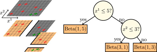
FIGURE 1. Example of a Bayesian Decision Tree for a 2-categories example in
In an attempt to build explainable Bayesian Decision Trees, we define a greedy construction that does not apply Markov Chain Monte Carlo. This construction balances the greedy approach from [6] with the Bayesian approach discussed in [9, 14–17]. For this, we compute the probability of each split at every node and choose the modal split. This results in a model that performs well with different data sets as shown in Section 4.
3 From the Partition Probability Space to Bayesian Decision Trees
The building block of the GMT algorithm is the partition probability space. For this space, we only consider binary partitions of the form
The partition probability space is the finite probability space defined by partitions
We will also need the feature sorted indices of the input features for computation and visualization purposes, namely
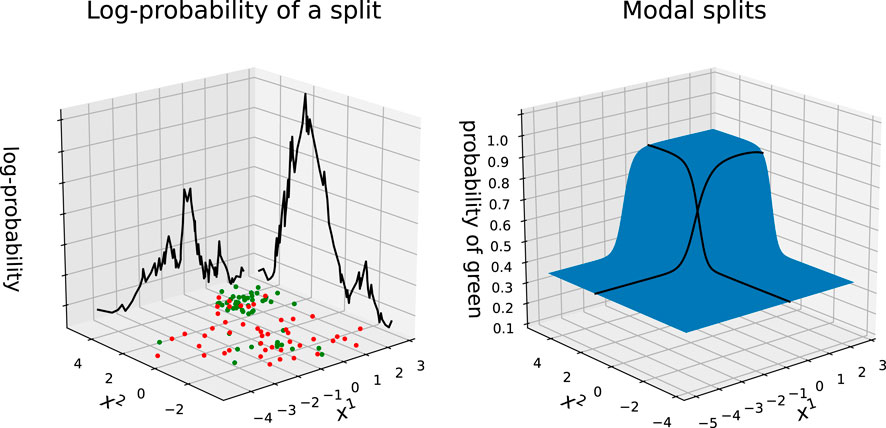
FIGURE 2. Example of a data set whose outcomes are either green or red. The location of the points is sampled from a mixture of two Gaussian distributions with equal probability. One distribution draws outcomes from a Bernoulli distribution with probability 0.25, while the other from a Bernoulli with probability 0.75. On the left: log-probabilities of all possible non-trivial partitions given the data set. On the right: actual probability of a point being green and modal splits along each dimension.
Each partition
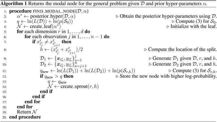
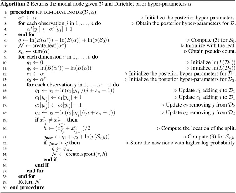
With the partition space and modal node defined, we can introduce the GMT construction. We start by finding the modal node
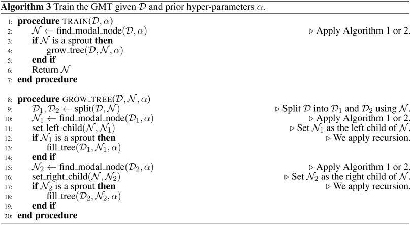
The average cost of Algorithm 3 is
4 Benchmark
4.1 Decision Trees, Random Forests, XGBoost, and GMT
In this Section we use Algorithm 2 and 3 to construct the GMT. We assume that the outcomes, 0 or 1, are drawn from Bernoulli random variables. The prior distribution
The accuracy is measured as a percentage of the correct predictions. Each prediction will simply be the highest probability outcome. If there is a tie, we choose the category 0 by default. We compare the GMT results to DT [6, 19], RF [11, 19], and XG [12]. For reproducibility purposes, we set all random seeds to 0. In the case of RF, we enable bootstrapping to improve its performance. We also fix the number of trees to five for RF and XG. We provide the GMT Python module with integration into scikit-learn in [20].
We test the GMT on a selection of data sets from the University of California, Irvine (UCI) database [21]. We compute the accuracy of the DT, RF, XG, and GMT with a shuffled 10-fold cross validation.We do not perform any parameter tuning and keep the same
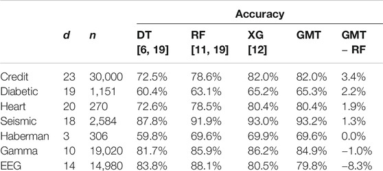
TABLE 1. Accuracy of DT, RF, XG, and GMT for several data sets. We apply a shuffled 10-fold cross validation to each test. Results are sorted by relative performance, starting from hightest accuracy difference between GMT and RF.
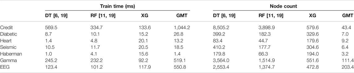
TABLE 2. Training time in milliseconds and average node count per fold. The node count includes the number of leaves.
The results reveal some interesting properties of the GMT. Noticeably, the GMT seems to perform well in general. In all cases, the DT accuracy is lower than the RF accuracy. The only case in which RF considerably outperforms the GMT is with the EEG data set. One reason may be that some information is hidden at the lower levels, i.e. feature correlation information that is hard to extract by looking at only one level ahead. The accuracy difference between GMT and RF indicates that these two techniques may work well for different data sets. Interestingly, the XG and GMT yield similar accuracies. Finally, in most cases the GMT takes more time to train than the other three techniques which is caused by the feature sorting overhead computation. Notably, the node count in Table 2 shows that we successfully managed to simplify the models while producing similar accuracy. Note that for four of the seven data sets, the average number of nodes is less than ten and produces slightly better accuracies than RF. Ten nodes implies less than five sprouts in average which can be easily analyzed by a human. This highlights the importance of the priors
4.2 Bayesian Decision Trees and GMT
In this section we analyze the GMT on the Wisconsin breast-cancer data set studied in [9, 14] which is available at the University of California, Irvine (UCI) database [21]. Although this data set contains 699 observations, we are going to use the 683 that are complete. Each observation contains nine features and the outcome classifies the tumor as benign or malignant. We test the GMT for
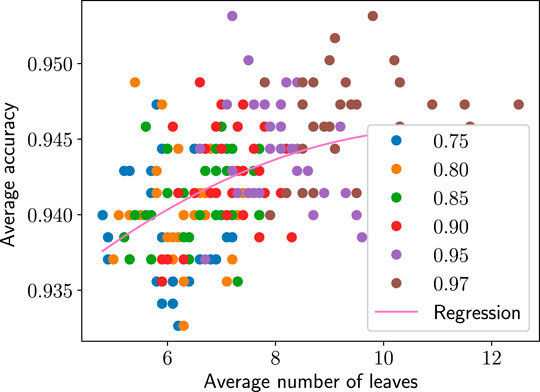
FIGURE 3. Average accuracy vs. average number of leaves for each GMT parameter set applied to the Wisonson breast-cancer data. The color indicates which parameter
5 Trading Example
We consider three stocks, A, B, and C, whose price follows a multidimensional Ornstein-Uhlenbeck process, [22]. Using the notation from [22], we can sample the prices by applying the Euler’s discretization,
Our goal is to train the GMT to predict the best portfolio configuration. Given that we have three stocks, we consider the following eight buy/sell configurations: +A/−B/−C (buy one stock A, sell one stock B, sell one stock C), −A/−B/−C, −A/+B/−C, +A/+B/−C, −A/−B/+C,+A/−B/+C, -A/+B/+C, +A/+B/+C. At each time step, we take the three stock prices
We treat this problem as an eight class classification problem. The GMT is trained with the
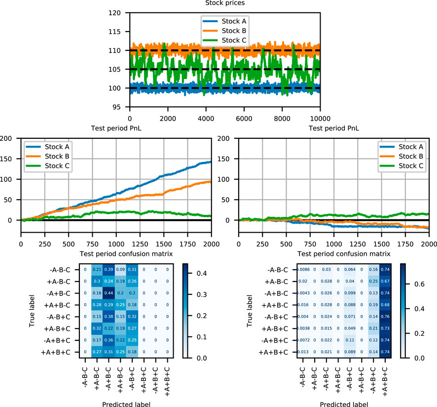
FIGURE 4. From top to bottom, left to right: Simulated stock prices, test period PnL (Profit and Loss) for the GMT, test period PnL for the neural network, confusion matrix for the GMT, and confusion matrix for the neural network. The PnL is the cumulative profit achieved when the predicted portfolios are executed. The costs are omitted for simplicity.
The GMT we obtained by training on the first 8,000 observations has only four leaves: if the price of stock A is below 99.96 and the price of stock B below 109.85, we choose + A + B − C; if the price of A is below 99.96 and the price of B above 109.85, we choose + A-B-C; if the price of A is above 99.96 and the price of B below 110.14, we choose −A + B − C; and if the price of A is above 99.96 and the price of B above 110.14, we choose −A − B + C. Although the mean reversion for stock C is not captured in this model, we successfully recovered simple rules to trade the mean reversion of A and B. Since the price of C is more volatile by Eq. 4, the current price of C is not enough to recover the mean reversion decision logic. Some filtering of the price of C would allow to capture its mean reversion. In the neural network case, the over-parametrization makes it difficult to recover this simple model.
The deterministic nature of Algorithm 3 provides a practical framework to explain how was the GMT constructed. We look at each of the nodes to understand how were the modal nodes chosen. The resulting GMT model contains three sprouts—node 0, node 1, node 2—and four leaves—node 3, node 4, node 5, node 6. Figure 5 shows the log-probability 3) of splitting our data-set at a particular price by stock for the three sprouts. At the root level, node 0, we consider the whole data set. In this case, one can increase the GMT likelihood the most by choosing
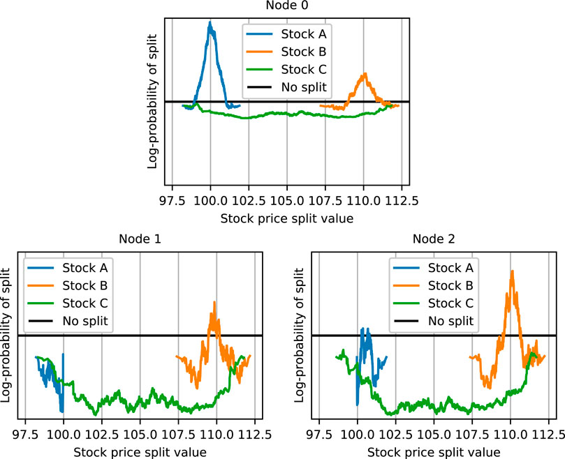
FIGURE 5. Log-probability of
6 Discussion and Future Work
The proposed GMT is a deterministic Bayesian Decision Tree that reduces the training time by avoiding any Markov Chain Monte Carlo sampling or a pruning step. The GMT numerical example results show similar accuracies to other known techniques. This approach may be most useful where the ability to explain the model is a requirement. Hence, the advantages of the GMT are that it can be easily understood. Furthermore, the ability to specify
As an extension, we would like to assess the performance of this algorithm on regression problems and experiment with larger partition spaces such as the SVM hyperplanes. Another computational advantage not explored is parallelization, which would allow for a more exhaustive exploration of the tree probability space from Eq. 1.
Data Availability Statement
The datasets presented in this study can be found at https://archive.ics.uci.edu/ml/datasets.php. The code is available at https://github.com/UBS-IB/bayesian_tree/.
Author Contributions
GN was the technical advisor leading the project. LlAJR was responsible for the technical details, first implementation, running the experiments, and manuscript preparation. AIC contributed in the manuscript preparation.
Funding
Authors were employed by UBS during the development of the project. UBS was not involved in the study design, collection, analysis, interpretation of data, the writing of this article or the decision to submit it for publication.
Conflict of Interest:
The authors declare that the research was conducted in the absence of any commercial or financial relationships that could be construed as a potential conflict of interest.
Acknowledgments
The authors want to thank Kaspar Thommen for the Python module implementation with integration to scikit-learn and his suggestions to improve the quality of this project. This manuscript has been released as a pre-print at https://arxiv.org/pdf/1901.03214, [23].
References
1. Lipton, ZC. The mythos of model interpretability. Queue (2018). 16:31–57. doi:10.1145/3236386.3241340
2. Herman, B. The promise and peril of human evaluation for model interpretability (2017). Preprint: arXiv: abs/1711.07414.
3. Doshi-Velez, F, and Kim, B. Towards a rigorous science of interpretable machine learning (2017). Preprint: arXiv:1702.08608.
4. Lipton, ZC. The doctor just won’t accept that! (2017). Preprint: arXiv:1711.08037.
5. Murdoch, WJ, Singh, C, Kumbier, K, Abbasi-Asl, R, and Yu, B. Definitions, methods, and applications in interpretable machine learning. Proc Natl Acad Sci USA (2019). 116:22071–80. doi:10.1073/pnas.1900654116
6. Breiman, L, Friedman, J, Stone, C, and Olshen, R. Classification and regression trees. The wadsworth and brooks-cole statistics-probability series. Abingdon, UK: Taylor and Francis (1984).
7. Quinlan, JR. C4.5: programs for machine learning. San Francisco, CA: Morgan Kaufmann Publishers Inc. (1993).
8. Friedman, JH. Greedy function approximation: a gradient boosting machine. Ann Stat (2000). 29:1189–232. doi:10.1214/aos/1013203451
9. Linero, AR. A review of tree-based Bayesian methods. Csam (2017). 24:543–59. doi:10.29220/csam.2017.24.6.543
12. Chen, T, and Guestrin, C. XGBoost: a scalable tree boosting system in Proceedings of the 22nd ACM SIGKDD international conference on knowledge discovery and data mining. New York, NY: ACM (2016). p. 785–94. doi:10.1145/2939672.2939785
14. Chipman, HA, George, EI, and McCulloch, RE. Bayesian CART model search. J Am Stat Assoc (1998). 93:935–48. doi:10.1080/01621459.1998.10473750
15. Denison, DGT, Mallick, BK, and Smith, AFM. A Bayesian CART algorithm. Biometrika (1998). 85:363–77. doi:10.1093/biomet/85.2.363
16. Chipman, HA, George, EI, and McCulloch, RE. Bart: Bayesian additive regression trees. Ann Appl Stat (2010). 4:266–98. doi:10.1214/09-AOAS285
17. Schetinin, V, Jakaite, L, Jakaitis, J, and Krzanowski, W. Bayesian decision trees for predicting survival of patients: a study on the us national trauma data bank. Comput Methods Programs Biomed (2013). 111:602–12. doi:10.1016/j.cmpb.2013.05.015
18. Gelman, A, Carlin, J, Stern, H, Dunson, D, Vehtari, A, and Rubin, D. Bayesian data analysis. 3rd ed. Boca Raton, FL: Chapman and Hall/CRC Texts in Statistical Science (Taylor & Francis) (2013).
19. Pedregosa, F, Varoquaux, G, Gramfort, A, Michel, V, Thirion, B, Grisel, O, et al. Scikit-learn: machine learning in Python. J Machine Learn Res (2011). 12:2825–30. doi:10.5555/1953048.2078195
20. Thommen, K, Goswami, B, and Cross, AI. Bayesian decision tree (2019). Available at: https://github.com/UBS-IB/bayesian_tree.
22. Vatiwutipong, P, and Phewchean, N. Alternative way to derive the distribution of the multivariate Ornstein-Uhlenbeck process. Adv Differ Equ, 2019 (2019). 2019. doi:10.1186/s13662-019-2214-1
23. Nuti, G, Jiménez Rugama LlA, , and Cross, A-I. A Bayesian decision tree algorithm (2019). Preprint: arXiv: abs/1901.03214
Keywords: explainable machine learning, Bayesian statistics, greedy algorithms, Bayesian decision trees, white box
Citation: Nuti G, Jiménez Rugama LIA and Cross A-I (2021) An Explainable Bayesian Decision Tree Algorithm. Front. Appl. Math. Stat. 7:598833. doi: 10.3389/fams.2021.598833
Received: 25 August 2020; Accepted: 12 January 2021;
Published: 22 March 2021.
Edited by:
Victor Wu, Tilt Dev, United StatesReviewed by:
Xiangyu Chang, Xi’an Jiaotong University, ChinaChandan Gautam, Indian Institute of Science, India
Marcela Svarc, Universidad de San Andrés, Argentina
Copyright © 2021 Nuti, Jiménez Rugama and Cross. This is an open-access article distributed under the terms of the Creative Commons Attribution License (CC BY). The use, distribution or reproduction in other forums is permitted, provided the original author(s) and the copyright owner(s) are credited and that the original publication in this journal is cited, in accordance with accepted academic practice. No use, distribution or reproduction is permitted which does not comply with these terms.
*Correspondence: Lluís Antoni Jiménez Rugama, bGx1aXMuamltZW5lei1ydWdhbWFAdWJzLmNvbQ==