 Ted G. Lewis
 Waleed I. Al Mannai
95% of researchers rate our articles as excellent or good
Learn more about the work of our research integrity team to safeguard the quality of each article we publish.
Find out more
ORIGINAL RESEARCH article
Front. Appl. Math. Stat. , 29 March 2021
Sec. Mathematics of Computation and Data Science
Volume 6 - 2020 | https://doi.org/10.3389/fams.2020.611854
This article is part of the Research Topic Modeling Epidemics - Why Are Models Wrong? View all 8 articles
This article explores the ongoing COVID-19 pandemic, asking how long it might last. Focusing on Bahrain, which has a finite population of 1.7M, it aimed to predict the size and duration of the pandemic, which is key information for administering public health policy. We compare the predictions made by numerical solutions of variations of the Kermack-McKendrick SIR epidemic model and Tsallis-Tirnakli model with the curve-fitting solution of the Bass model of product adoption. The results reiterate the complex and difficult nature of estimating parameters, and how this can lead to initial predictions that are far from reality. The Tsallis-Tirnakli and Bass models yield more realistic results using data-driven approaches but greatly differ in their predictions. The study discusses possible sources for predictive inaccuracies, as identified during our predictions for Bahrain, the United States, and the world. We conclude that additional factors such as variations in social network structure, public health policy, and differences in population and population density are major sources of inaccuracies in estimating size and duration.
This study seeks to answer questions regarding how long the COVID-19 pandemic will last in the Kingdom of Bahrain and what will its final size be? Predicting size and duration is key to administering public health policy. This is a challenging problem, especially for COVID-19, because of different policies in different regions, differences is population/population density, and underlying network effects. Classical models such as the Kermack-McKendrick model have proven to be inadequate.
We limit our study to Bahrain and the United States. Bahrain is an ideal laboratory for studying epidemics because it is a comparatively isolated island with a small homogeneous population of 1.7 million people. In addition, it has collected reliable data on the outbreak of COVID-19 that can be used by data-driven models. Restrictions are strictly enforced: people have to wear masks or be ticketed for violating the law. The restaurants and coffee shops are closed and only takeout is allowed. The mosques are closed too. Only five people are allowed to gather in one place.
The study examines three classes of models, including the classical Kermack-McKendrick (KM), Tsallis- Tirnakli, Bass Model, which were chosen for their variety. KM, or variants of KM, provide a baseline [1]. The novel Tsallis-Tirnakli model was chosen for its fresh complexity approach, and the Bass model because it comes from an entirely different application: product adoptions. However, all three classes share a basic premise - they assume spreading via contact, and mathematically, they all assume curve fitting to obtain the model parameters.
This study examines which models perform the best in terms of providing accurate estimates of size and duration so that we can have confidence in scientific predictions the next time an epidemic or pandemic strikes. Mathematical models are used to investigate and understand the dynamics of outbreaks of infectious diseases in humans, such as SARS, Ebola, and COVID-19. It is important to ensure that these models are accurate as they provide public health sector policymakers with forecast information to help them plan, including estimates relating to the medicines, number of beds, and medical equipment required. Accurate modeling is also essential in applying countermeasures to control and end the pandemic. Therefore, it is imperative that policymakers are able to predict the size and duration of an epidemic with precision.
In an article published on April 29, 2020, researchers predicted that the number of cases and deaths would exceed 60,000 in the United States by July: “we estimate that through the end of July, there will be 60,308 (34,063–140,381) deaths from COVID-19 in the USA …” [13]. The number of deaths exceeded 100,000 by April 26, 2020 and continued to climb, surpassing the upper bound on the estimate by late June 6, 2020. This illustrates one problem with existing models.
Problems with estimations often occur due to missing factors that account for all impacts in the models. “Each model makes different assumptions about properties of the novel coronavirus, such as how infectious it is and the rate at which people die once infected. They also use different types of math behind the scenes to make their projections. And perhaps most importantly, they make different assumptions about the amount of contact we should expect between people in the near future.”1 See Table 1.
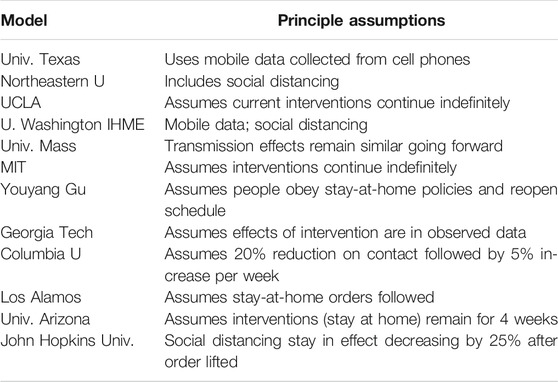
TABLE 1. Summary of contemporary models in the fight against COVID-19.1
In this article, we claim that the problem of estimating size and duration extends beyond assumptions about properties of the disease and infectiousness. We show that, in addition to the limitations expressed above, population, population density, social network topology, and public sentiment impact the rate and size of the spread of a disease. Mathematical models based solely on properties of the disease are likely to fail, whereas models based on curve-fitting of data and social network theory and public sentiment are more likely to succeed. However, these models fail to accurately predict the size and duration of the COVID-19 pandemic due to a number of technical, social, and public policy issues.
Most models assume a uniformly distributed population with the same levels of immunity or susceptibility to infection and a relatively immobile population. However, the modern world does not always follow all of these conditions. For example, populations are clustered, people of different ages and economic conditions have different susceptibilities to diseases, public opinion as to the dangers of contagion shift over time, and people are extremely mobile.
Historically, epidemic spreading has been formulated as a rate problem similar to the flow of a fluid or conduction of heat. One must know the infection rate to model the spread of the contagion and the removal rate to model deaths and cures. At this point, models split into persistent and not. A persistent epidemic recurs because the infection rate is larger than the removal rate. This is considered SIS (susceptible-infected-susceptible). In contrast, the SIR model is episodic (susceptible-infected-recovered). Once the infection and recovery/removal rates are known, the equations take over—no data from actual epidemics are used to make predictions.
Flow models are inadequate at representing what goes on in modern society. Populations are more mobile, concentrated, and social, making it difficult to model epidemics as flows. Instead, modern models use diffusion equations and complexity equations to represent the spread of a contagion. Moreover, these models are much more data-driven because conditions change. For example, social distancing, patterns of mobility, and nonuniform mixing affect the contagion, causing it to surge in some places and die out in other places, which can only be represented in the data. However, flow models like the Kermack-McKendrick (KM) model provide a benchmark for comparison purposes. More recently, network-based models have been used to relate the structure of a social network with the spread of a contagion along social links [5].
In this research, we compare three models: the classic two-parameter SIR model given by Kermack-McKendrick, the 5-parameter Tsallis-Tirnakli complexity model, and the 3-parameter Bass model, which was developed to study the diffusion of innovation in consumer products. While the Bass model is designed for product adoption, its diffusion process is similar to the diffusion of germs in epidemiology. We conclude the study by identifying limitations and missing factors that need to be considered by mathematical models in general.
In 1927, W. O. Kermack and A. G. McKendrick (KM) developed the first mathematical model describing the spread of epidemics [2, 4]. Over the past 90 years, various derivatives of the KM models have appeared, for example, the SEIR model that separates susceptible populations from exposed, infected, and recovered populations. In addition to historical interest, KM is a simplistic model that provides a basis for comparison with newer and more sophisticated models.
The basic KM model divides the fixed-size population into three compartments: susceptible, infected, and recovered or removed (SIR). The total population of M people is constant, but the subject flows from one compartment to another:
The rate of flow into and out of each compartment is determined by two constant parameters: ɣ = rate of infection and ß = rate of recovery (or removal). The values of the two parameters must be estimated quite carefully; otherwise, the result will be inaccurate. In fact, small errors in the initial conditions will result in large errors in the solution. This is the Achilles heel of KM.
The rate of change in the number of people susceptible to the disease over time is given by the following:
The rate of change of the number of people recovered over time is as follows:
The rate of change of the number of people infected is as follows:
With the initial condition,
where S is the number of susceptible people to COVID-19; I is the number of people infected with COVID-19; R is the number of people removed (or recovered);
Following [6], we use numerical methods to solve for S(t), I(t), and R(t). Unfortunately, estimating
Raissi et al. [9, 12] used filtering techniques to compute values of the parameters by averaging over the data. The technique is very sophisticated and introduces additional parameters. Our goal is to reduce the number of parameters to a minimum.
The results reported in this article used curve-fitting to actual data to estimate
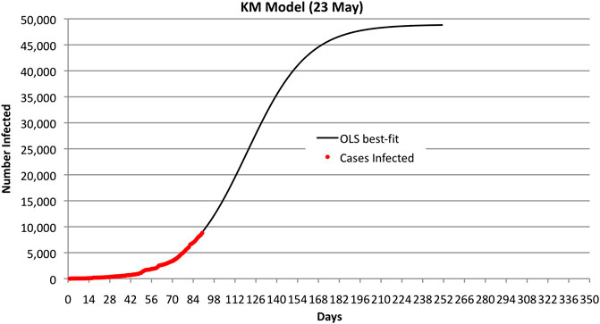
FIGURE 1. Bahrain KM OLS best fit and observed number of infected cases through 23 May 2020. Note that the curve predicts 50,000 cases.
In practice, one is typically interested in the total number of infected cases, which simplifies the analysis and leads to a sigmoid function first proposed by Pierre Francois Verhulst (1804–1849). In this model, a population is separated into two compartments: susceptible and infected. The differential equation reduces to the following:
This equation has a three-parameter solution:
where N is the size of the epidemic, to be determined or given; K,
The Tsallis-Tirnakli model is based on a complexity theory and statistical mechanics applied to stocks; “the time evolution of the number I(t) of active cases (surely a lower bound of the unknown actual numbers) showed a rather intriguing similarity with the distributions of volumes of stocks [10].” It is derived from the q-distribution, which is a fat-tailed pseudo-normal distribution [11].
To estimate size and duration, one must plot I(t) vs. time using the following equation:
The model depends on 5 parameters: “C > 0, a > 0, ß > 0, γ > 0, q > 1, and t0 ≥ 0. The constant t0 indicates the first day of appearance of the epidemic in that particular region; it is conventionally chosen to be zero for China; for the other countries, it is the number of days elapsed between the appearance of the first case in China and the first case in that country. The normalizing constant C reflects the total population of that particular country. For a = 0, if γ = 1, we recover the standard q-exponential expression; if γ = 2, it is currently referred to in the literature as q-Gaussian; for other values of γ, it is referred to as stretched q-exponential. Through the inspection of the roles played by the four nontrivial parameters, namely (α, β, γ, q), it became clear that (α, β) depend strongly on the epidemiological strategy implemented in that region in addition to the biological behavior of the coronavirus in that geographical climate. In contrast, the parameters (γ, q) appear to be more universal, mainly depending on the coronavirus. Therefore, we investigate several countries that have not reached their peaks yet, with the basic assumption that these two parameters would not change much from one country to another, and we fixed these values at the values that we determine for China, since this country has already had nearly the full evolution of the pandemic.”
The equation is deceptively simple, but the parameters are difficult to come by because they are guesses. Parameters may be reused from other epidemics; for example, two parameters appear to be universal at approximately q = 1.26 and γ = 3. But, values of C range from 10–3 to 10–8; t0 range from 10 days to 48, etc. It is a tedious process to find the best-fit to time series epidemic data.
Figure 2 shows the parameters used to fit the Bahrain COVID-19 data obtained by trial and error. These values were obtained after a few hours of experimentation by hand and running a computer program to compute OLS.
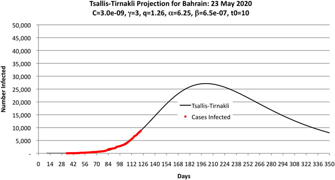
FIGURE 2. Parameters used by the authors to fit the COVID-19 data as of 23 May 2020 (shown as black dots) to the Tsallis-Tirnakli distribution. Note that the curve predicts 33,000 cases.
An unrelated mathematical model developed by Frank M. Bass in 1969 is simple and precise in predicting sales of new products [3, 4]. The Bass model estimates the total size of the market and when peak sales occur, called the inflection point, from actual data collected on sales [7]. The advantage of the Bass model is that the parameters that determine size and duration are easily computed by fitting a quadratic to the infection time series data.
As long as we accept diffusion of products as a suitable model for the spread of a contagion, we can use the simple and elegant solution provided by Bass. The Bass equation does not subtract the recovered cases from the infected, so the Bass curve is a pure logistics curve. But it can still be used to estimate N and time to reach N.
The Bass differential equation, as defined in [7], gives the cumulative number of infected people without removal. Since we are interested in the size and duration of an outbreak, this is not a limitation. Instead, it is a simplification.
which has the following closed-form solution:
where
s is the rate of spreading used in the differential equation [7]; S is the cumulative number of cases infected in [7]; N is the ultimate size of cumulative cases, not the susceptible population; p is the rate of infection called the innovation parameter by Bass; q is the secondary rate of infection called the imitation parameter by Bass.
The first attempt to apply the Bass model to infectious disease was an extended model by Gupta [8]. He introduced an additional parameter called the outcome rate for forecasting the spread of the pandemic. The outcome rate consists of a cure rate and a death rate, but does not help one to estimate size and duration. However, the application of the Bass model is similar to the method used here.
A later adaptation of the Bass model, called Bass-SIR, was proposed by Ku, Ng, and Lin in January 2020 [19]. As the name implies, it combines product adoption and infectious disease spreading but does not answer the fundamental question addressed here, which is the accuracy of size and duration.
The Bass model is data-driven and requires only three parameters to estimate how long COVID-19 will last and its final size without making assumptions about a particular disease or borrowing parameters from previous outbreaks. It is not necessary to solve the Bass equation in order to estimate the size and duration of the outbreak. Instead, Eq. 7 can be rewritten in quadratic form as follows:
or
where A = Np, B = q–p, and C = −q/N.
The parameters A, B, and C can be estimated using least-squares fitting to the evolving data, as shown in Figure 3. That is, Figure 3 plots s against S, where S is cumulative data and s is data collected on a daily basis. The actual data are fit to a quadratic equation to obtain A, B, and C. The parameters p, q, and N can be determined from A, B, and C as follows:
and
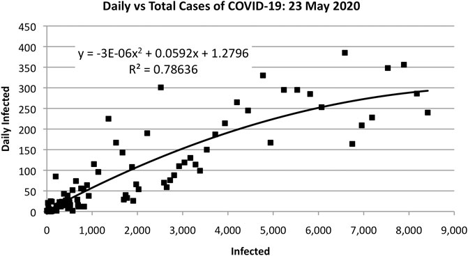
FIGURE 3. Applying the quadratic Bass model to predict 28,360 total cases as of 23 May 2020.
In addition, since we know the solution to the Bass differential equation a priori, we can find the time to reach the inflection point, t*. This is the point in time when the new infections peak and the curve begins to bend downward.
The Tsallis-Tirnakli model declines after reaching a peak because it incorporates removed cases due to death or recovery, whereas the Bass and KM model count only total infected (including removed).
A second wave hit Bahrain on the third of September 2020 (day 193), as shown in Figure 4, where there is a steep increase in the actual cases infected. All three models did not predict this sudden increase accurately. In addition, there is a big difference between the prediction and actual values. Figure 5 indicates that the models either overestimated or underestimated. The interval is between [−36,800, 8,350] cases infected – a very large difference. See Table 2.
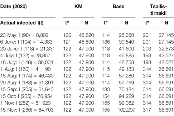
TABLE 2. Bahrain results for KM, Tsallis-Tirnakli, and Bass models show Divergent size and duration estimates.
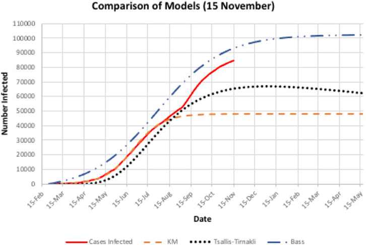
FIGURE 4. All three Bahrain models failed to detect the second wave on September 3rd.
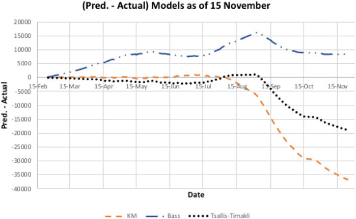
FIGURE 5. Underestimated/overestimated Model prediction for Bahrain data. However, the Bass model appears to converge to a better estimate of size than the other two models.
There are many explanations for why epidemic models fail to predict the size and duration of outbreaks. We list only a few here. First, these models assume uniform mixing of the population, but we know that human populations form clusters, which result in surges of infection as it spreads from cluster to cluster. Second, the models do not incorporate the effects of mitigation strategies such as social distancing or quarantine. In addition, they all assume that the infection rate is constant and the same for all individuals, when we know that the infection rate varies with age and occupation. Finally, they assume that people follow public health policy advice, but we know that public sentiment often overrides policy advice, as demonstrated in the United States by a rise in cases after relaxing social distancing and the wearing of masks.
The models compared here are difficult to use because, in addition to assumptions about uniform mixing and uniform susceptibility to diseases, they require an accurate estimate of parameters subject to adjustment as more data are collected. For example, in [6], the researchers found that variation in the estimate of initial conditions for the KM equations leads to great inaccuracy in the resulting numerical solution. They had to adjust the calculated values using curve-fitting to obtain reasonable projections of the spread of Ebola. Yet, KM did as well as the other two models for the Bahrain case study.
When applied to pandemic-scale contagions, these models often fail to scale up. For example, for worldwide COVID-19 spreading, the Bass model predicted N = 35 million on 23 May; 14 million on 6 June; three million on 20 June; 4.6 million on July 4, 2020. On July 15, the actual number was 13.5 million and increasing. The Tsallis-Tirnakli model does better but gives only orders of magnitude estimates for N and fails to estimate duration. For example, it estimated US cases would peak around July at 106, but as of July, the number of actual cases surpassed 3.5 million and was accelerating. In Brazil, Tsallis-Tirnakli underestimated the number of cases by millions. However, Tsallis-Tirnakli accurately estimated the size of COVID-19 for European nations as they reached 105 cases.
Generally, epidemic models do not scale well for estimating the size and duration of pandemics because of diverse populations, policies, and social structures. We examine three impactful factors as follows: population, mobility, and social network structure and quarantine policy.
Large populations have more cases of infection than small populations, but do large populations affect the number of cases per capita more than small populations? To address this question, the authors compared the population of the 50 states of the United States with the number of infected cases known on July 4, 2020. The population of US states ranges from 528,000 (Wyoming) to 39.5 million (California).
A log-log plot of the frequency of infected cases vs. cases/100,000 population is shown in Figure 6. The data are placed into bins of equal size and a straight line fit to the log-log graph. The slope of this line q is the exponent of a power law ∼1/xq. That is, the number of cases per capita x obeys a power law rather than a normal distribution, which suggests that cases were not random across different regions of the US. Cirillo and Taleb observed a similar “fat tail” distribution of epidemic [fatalities] throughout recorded history. “We show that pandemics are extremely fat-tailed in terms of fatalities, with a marked potentially existential risk for humanity,” when examining data over the past 2,500 years [17].
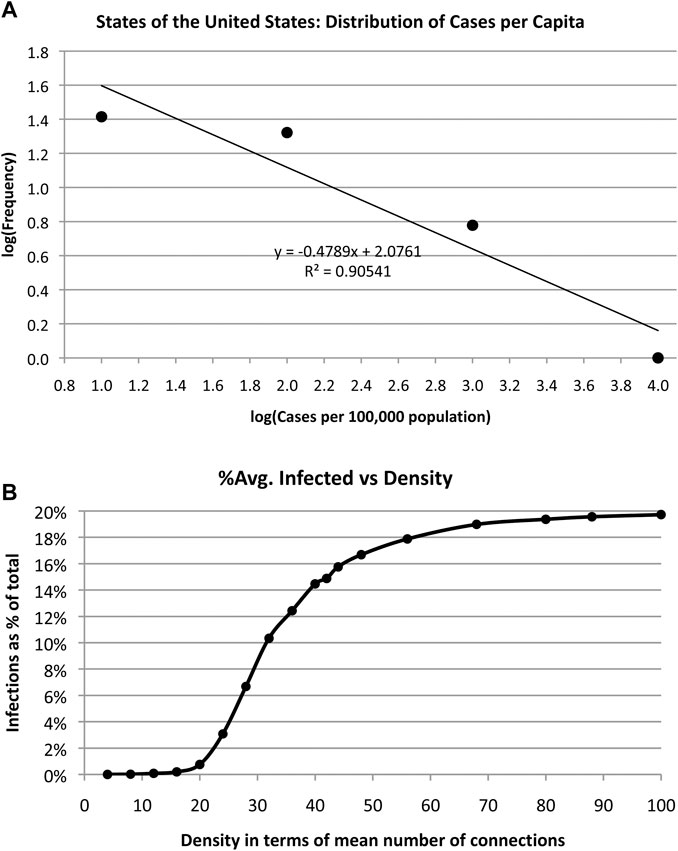
FIGURE 6. (A) The distribution of COVID-19 spreading obeys a power law vs. the number of cases per capita as shown in this log-log plot. (B). Simulation of average number of infections in a random network of 500 actors and 5% infection rate shows that number of infections increases with density of network links.
Similar power law relationship exists for individual states at one extreme and at a global level at the other extreme. The exponents of the power laws obtained for all countries of the globe, the US, and Texas are summarized in Table 3. This means that size of the epidemic is unpredictable but not random. N varies according to a long-tailed distribution.
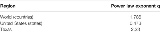
TABLE 3. Distribution of cases per capita obey power laws.
Note that if cases per capita determined N alone, the curve in Figure 6 would not fit a power law—the frequency distribution would be a flat line with a slope of zero, assuming infections per capita are constant. The fact that N is distributed according to a power law indicates that public sentiment, different policies in different regions, and different social structures all play a role in determining N. It also suggests that N is an unpredictable parameter.
Next, we examine the impact of size of social group with random contacts on number of infections by simulating random networks with 500 nodes and varying densities. We define density as the average number of connections per node. That is, we vary the number of random links from 1,000 to 24,000 and run 10,000 simulations each to arrive at an average number infected assuming an infection rate of 5%. See Algorithm 1.
The results are shown in Figure 6(b) indicating an increasing number of infections as the density increases, as expected. Social distancing and small crowds are effective counter measures to infection. Alternatively, increasing density has the same effect as increasing the infection rate. The more contact people make, the more likely it is that they will become infected. The simulation merely quantifies common sense.
Most populations of the countries of the world are fluid—they are in constant motion. We can study this by analyzing transportation networks and their weak ties to other regions. Transportation networks link population clusters together to form larger “mega-clusters” of people susceptible to disease. Transportation networks introduce time delays and surges into the model.
Consider two transportation networks–—the global commercial airline network called Openflight2 and a regional network such as the Los Angeles Metro commuter system. Openflight contains 3,425 airport nodes and 19,256 unique routes connecting the airports. It is extremely interconnected with a cluster coefficient of 0.48. The LA Metro network, in contrast, contains 117 stations connected by 127 railroads, with a cluster coefficient of 0.018. Openflight is “bushy,” whereas LA Metro is “branchy,” so we expect them to transmit viruses differently from one another. These networks are shown in Figure 7. Bushy vs. branchy networks are more formally defined as small diameter large spectral radius (bushy) vs. large diameter small spectral radius (branchy). Scale-free networks are extremely bushy with relatively large spectral radius.
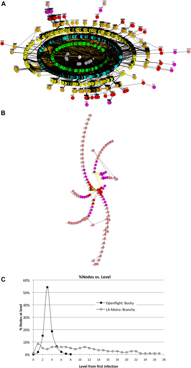
FIGURE 7. Two contrasting transportation networks: (a) the Openflight network with 3,425 airports and the LA Metro with 117 stations. Infection rate v = 50%. (A). Openflight network in Wuhan, China. (B). LA Metro network in Union Station in downtown Los Angeles. (C). Distribution of nodes across levels differs greatly for bushy Openflight vs. branchy LA Metro. This has a direct impact on the size and duration of epidemics.
The authors simulated the spread of COVID-19 through both networks starting at Wuhan with 66 connections for Openflight and Union Station with 10 connections for LA Metro. Ten thousand runs were averaged to determine the frequency of occurrences of size, N. The simulated contagion algorithm is given in Algorithm 1.
In each case, the first thing to notice is that N varies, statistically, leading to histograms, as shown in Figure 8. The branchy topology of the LA Metro network reduces its susceptibility to infection, although peak N varies widely from 0 to 40%. Openflight, on the other hand, is more likely to infect a higher fraction of the total due to population clusters at each node. Assuming the number of infected is equal to the degree of each node shifts the size of N from 75 to 95%.
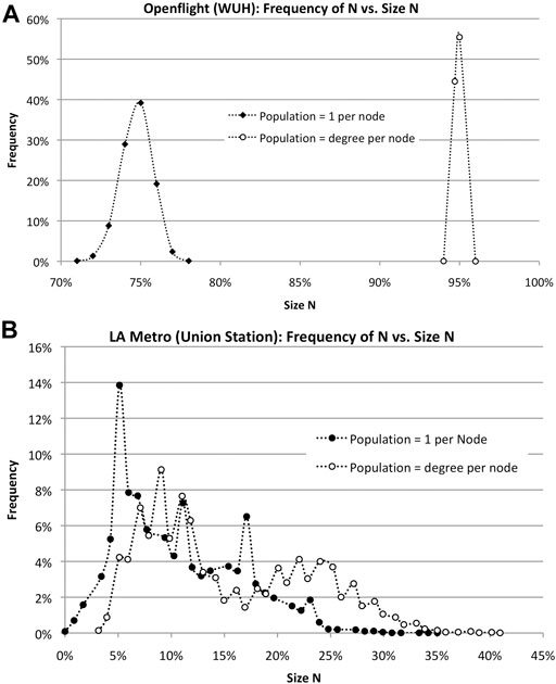
FIGURE 8. Simulations of epidemics in travel networks Openflight and LA Metro show vast differences in peak N for different assumptions about population. (A). Openflight size of outbreak N varies depending on the population at each node: one vs. the degree of the node. The horizontal axis is the percentage of the total number of nodes. (B). LA Metro size of outbreak N varies depending on the population at each node: 1 vs. the degree of the node. In addition, the topology of the network–low clustering–vastly reduces the size N. Infection rate v = 50%.
Simulations of epidemics in hypothetical scale-free and random networks with identical spectral radius illustrate in a dramatic way how topology severely impacts contagion. When the spread of a contagion in a random network with a spectral radius of 9.0 is compared with a scale-free network also of a spectral radius of 9.0, the random network's N ranged from 96 to 99% of nodes infected vs. 59–85% of scale-free nodes infected assuming an infection rate of 50%.
This wide variation in N due to topology can be seen in the distribution of the number of nodes at different levels in Figure 7. Openflight has over 50% of its nodes at three levels from Wuhan, while LA Metro spreads 50% of its nodes over 10 levels—three times as many as Openflight.
It is clear that network topology and clustering have a major impact on the size of an epidemic. None of the models discussed in this article consider topology or clustering and yet these are factors that greatly affect size.
v: infection rate
L: link
L.visited = false for all L
Repeat until there are no more infections
Set t = 0
For every link L that has not been visited already do
If one end of L is infected, infect the other end with probability v
Mark L as visited (One-shot exposure)
End for
Count the number of nodes infected
Increment t
End repeat
The authors added quarantining to Algorithm 1 to obtain Algorithm 2: Quarantine. After each time step in the contagion spreading algorithm, scan the network nodes looking for clusters of size ≥ q, and when found, quarantine them. A cluster is defined as a node and all of its nearest neighbors. A cluster of size ≥ q is defined as a cluster with at least q infected neighbors.
Applying Algorithm 2 to the LA Metro and Openflight networks yields much better results. Instead of N = 5 and 75%, quarantining results in N = 2 and 20%, respectively, when clusters of size q = 3 are quarantined and N = 5 and 30%, respectively, when q = 5. As the size of the cluster rises, the effectiveness declines. This is due to allowing more nodes to infect other nodes as the contagion spreads. Clearly, quarantine strategies are effective and impact size and duration in positive ways that are not accounted for in most mathematical models. These results are for an infection rate of 50%.
The approach here depends on a known network. An alternate approach using machine learning techniques is proposed by Dandekar and Barbastathis [16] to find a quarantine function from outbreak data of COVID-19 in Italy, South Korea, and the United States. Known data are used to train a neural network “by training it from data in the January 24th till March 3rd window, and then matching the predictions up to April 1st [16].” Unfortunately, the neural network model is no better than curve-fitting models described here, “In the case of the US, our model captures well the current infected curve growth and predicts a halting of infection spread by 20 April 2020.” As of 20 April 2020, the outbreak was still going full force and continued its exponential growth into June.
v: infection rate
L: link
L.visited = false for all L
Repeat until there are no more infections
Set t = 0
For every link L that has not been visited already do
If one end of L is infected, infect the other end with probability v
Mark L as visited (One-shot exposure)
End for
Count the number of nodes infected
For every node j do
Count the number of neighbors infected, k
If k > q Quarantine(j) and its neighbors
End for
Increment t
End repeat
COVID-19 exhibits wave-like behavior—both in time and space. In time, many regions exhibited multiple peaks and valleys in recorded cases of infected people. In space, the peaks and valleys occurred in different countries and regions, seemingly in no apparent pattern. One explanation might be that peaks and valleys are caused by space and time shifts in terms of the start of “mini-epidemics” that spread through weak ties. This is illustrated in Figure 9A, which is based on high-frequency surges in Florida during the summer of 2020 and on low-frequency or long waves in California where there was a resurgence in the spread of COVID-19, see Figure 9B.
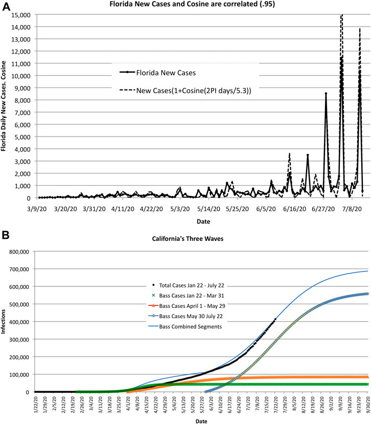
FIGURE 9. As COVID-19 encounters clusters of large populations, the estimate of size and duration increases. The error in these estimates may be caused by the time shift and magnitude of the infected clusters or shifts in public sentiment, as illustrated by the two examples shown here. (A). High-frequency wave-like behavior in Florida. The correlation coefficient between actual new cases and cosine waves is 0.95 for 5.3-day cycles. (B). Long wave-life surges in California caused by “mini-epidemics” recurring with different start times and amplitudes.
Villalobos and Alberto modified the Verhulst sigmoid to accommodate late-stage surges shown in Figure 9B [18]. Their 5-parameter model incorporates a time-dependent spread of COVID-19 as follows:
They argue, “if we have the lower part of the curve, that is, the first values of the curve, we can obtain the parameters of the curve, and obtain the complete curve. And with this it can be used to predict population growth, in this case, for example, the total number of cases by COVID-19 in a country or region and when the inflection point is reached, that is, when that the number of daily cases begins to decrease.”
The modification introduces additional parameters but gives exceptionally accurate size estimates for China and South Korea, which saw a slight resurgence on March 31, 2020. The parameters that give the best-fit (R2 = 0.9999) are listed below. But this model has no size or duration because I(t) can go to infinity when c > 0!
It is worth mentioning the two-stage model proposed by Katriel showing instabilities in social contagions that are reminiscent of bursts and instabilities in the spread of COVID-19 [20]. His novel solution introduces the idea of multiple stages of infection and offers an alternative to the explanations given here. The dynamic system model of Katriel is in contrast to the network science model given here.
The authors speculate that the global spread of COVID-19 is a Lévy Flight–a random walk with waypoints separated in space and time by a distance that obeys a power law. Lewis [14] estimated the exponent of the power law (1.6) that fit the distances traveled by SARS from country to country, confirming a theory of why SARS was stopped quickly [15]. If the Lévy Flight theory is correct and N depends on topology, the problem of estimating size and duration will remain until topology, geography, public sentiment, and population density are incorporated into our models.
Ted G. Lewis is an author, speaker, and consultant with expertise in applied complexity theory, homeland security, infrastructure systems, and early-stage startup strategies. He has served in both government, industry, and academe over a long career and held positions including Executive Director and Professor of Computer Science, Center for Homeland Defense and Security, Naval Postgraduate School, Monterey, CA. 93943; Senior Vice President of Eastman Kodak; President and CEO of DaimlerChrysler Research and Technology, North America, Inc; Professor of Computer Science at Oregon State University, Corvallis, OR. In addition, he has served as the Editor-in-Chief of a number of periodicals: IEEE Computer Magazine, IEEE Software Magazine, as a member of the IEEE Computer Society Board of Governors. He is currently an Advisory Board Member of ACM Ubiquity and Cosmos + Taxis Journal (The Sociology of Hayek). He has published more than 35 books, most recently including The Signal: A History of Signal Processing, Book of Extremes: The Complexity of Everyday Things, Bak's Sand Pile: Strategies for a Catastrophic World, Network Science: Theory and Practice, and Critical Infrastructure Protection in Homeland Security: Defending a Networked Nation, 3rd ed. Lewis has authored or coauthored numerous scholarly articles in cross-disciplinary journals such as Cognitive Systems Research, Homeland Security Affairs Journal, Journal of Risk Finance, Journal of Information Warfare, IEEE Parallel & Distributed Technology, Communications of the ACM, and American Scientist. Lewis resides with his wife and corgi dogs in Monterey, California.
Waleed I. Al Mannai served for 37 years in Bahrain Defense Ministry and retired as a colonel with extensive experience in military aviation aircraft, military operations, and academia. He received his Ph.D. in Modeling, Virtual Environments, and Simulation from the Naval Postgraduate School in Monterey, California; his M.S. in Aeronautical Engineering from the Naval Postgraduate School in Monterey, California; his B.S. in Aerospace Engineering from Northrop University in Los Angeles California. His areas of interest are Modeling and Simulation, Critical Infrastructure Protection (CIP) Network Risk, and Data Analysis and Managerial Decision Analysis.
The original contributions presented in the study are included in the article/Supplementary Material; further inquiries can be directed to the corresponding author.
KM developed equations and numerical solutions to models, gathered data, and provided graphs. TL extended the results to networks, e.g., OpenFlight and LA metro, and wrote the simulators. In addition, TL did the Bass model.
The authors declare that the research was conducted in the absence of any commercial or financial relationships that could be construed as a potential conflict of interest.
The Supplementary Material for this article can be found online at: https://www.frontiersin.org/articles/10.3389/fams.2020.611854/full#supplementary-material.
1Ryan Best, Jay Boice, Where The Latest COVID-19 Models Think We're Headed—And Why They Disagree (June 12, 2020). https://projects.fivethirtyeight.com/covid-forecasts/?ex_cid=rrpromo
2https://github.com/jpatokal/openflights/
1.Corona virus cases. (2020). Available from: https://www.worldometers.info/coronavirus/ (Accessed 2020).
2. Kermack, WO, and McKendrick, AG. A contribution to the mathematical theory of epidemics. Proc Royal Soc A (1927). 115:700–21. doi:10.1016/S0092-8240(05)80040-0
3. Bass, FM. A new product growth for model consumer durables. Manag Sci (1969). 15(5):215–27. 10.1287/mnsc.1040.0264
4. Gentry, L, and Calantone, R. Paper 662. Forecasting consumer adoption of technological innovation: choosing the appropriate diffusion models for new products and services before launch. Faculty Research & Creative Works (2007). Available at: http://scholarsmine.mst.edu/faculty_work/662 (Accessed 2007).
6. Hossain, T, Miah, M, and Hossain, B. Numerical study of Kermack-McKendrick SIR model to predict the outbreak of Ebola virus diseases using euler and RK4 methods. American Scient Res J Eng Tech Sci (2017). 37(1):1–21.
9. Raissi, M, Ramezani, N, and Seshaiyer, P. On parameter estimation approaches for predicting disease transmission through optimization, deep learning and statistical inference methods. Letters in biomathematics. Informa U.K., (2019).
10. Tsallis, C, and Tirnakli, U. Predicting COVID-19 peaks around the world. Front Phy (2020). 8:217. doi:10.3389/fphy.2020.00217
11. Osorio, R, Borland, L, and Tsallis, C. Distributions of high-frequency stock market. Nonextensive entropy: interdisciplinary applications (2004). 321.
12. Chen, Y-C, Lu, P-E, Chang, C-S, and Liu, T-H. (2020). A time-dependent SIR model for COVID-19 with undetectable infected persons. Available from: http://gibbs1.ee.nthu.edu.tw/A_TIME_DEPENDENT_SIR_MODEL_FOR_COVID_19.PDF (Accessed 2020).
13. Murray, C. Forecasting the impact of the first wave of the COVID-19 pandemic on hospital demand and deaths for the USA and European Economic Area countries. medrvix (2020). doi:10.1101/2020.04.21.20074732
15. Xu, RH, He, JF, Evans, MR, Peng, GW, Field, HE, Yu, DW, et al. Epidemiologic clues to SARS origin in China. Emerg Infect Dis (2004). 10(6):1030–7. doi:10.3201/eid1006.030852
16. Dandekar, R, and Barbastathis, G. Quantifying the effect of quarantine control in Covid-19 infectious spread using machine learning. medRxiv [preprint]. Available at: https://doi.org/10.1101/2020.04.03.20052084.t (Accessed 2020).
17. Cirillo, P, and Taleb, NN. Tail risk of contagious diseases. Nature Phys (2020). doi:10.1038/s41567-020-0921-x
18. Villalobos-Arias, M. Using generalized logistics regression to forecast population infected by Covid-19. (2020). Available from: https://arxiv.org/abs/2004.02406 (Accessed April 6, 2020).
19. Ku, C-C, Ng, T-C, and Lin, H-H. Epidemiological benchmarks of the COVID-19 outbreak control in China after Wuhan’s lockdown: a modelling study with an empirical approach. SSRN Elect J (2020). doi:10.2139/ssrn.3544127
Keywords: COVID-19, estimating epidemics, Kermack-Mckendrick, Tsallis-Tirnakli, Bass model, predicting cases, total cases, duration of epidemic
Citation: Lewis TG and Al Mannai WI (2021) Predicting the Size and Duration of the COVID-19 Pandemic. Front. Appl. Math. Stat. 6:611854. doi: 10.3389/fams.2020.611854
Received: 29 September 2021; Accepted: 07 December 2020;
Published: 29 March 2021.
Edited by:
Yiming Ying, University at Albany, United StatesReviewed by:
Halim Zeghdoudi, University of Annaba, AlgeriaCopyright © 2021 Lewis and Al Mannai. This is an open-access article distributed under the terms of the Creative Commons Attribution License (CC BY). The use, distribution or reproduction in other forums is permitted, provided the original author(s) and the copyright owner(s) are credited and that the original publication in this journal is cited, in accordance with accepted academic practice. No use, distribution or reproduction is permitted which does not comply with these terms.
*Correspondence: Ted G. Lewis, dGVkZ2xld2lzQGljbG91ZC5jb20=
Disclaimer: All claims expressed in this article are solely those of the authors and do not necessarily represent those of their affiliated organizations, or those of the publisher, the editors and the reviewers. Any product that may be evaluated in this article or claim that may be made by its manufacturer is not guaranteed or endorsed by the publisher.
Research integrity at Frontiers
Learn more about the work of our research integrity team to safeguard the quality of each article we publish.