Spatiotemporal Large-Scale Networks Shaped by Air Mass Movements

The movement of atmospheric air masses can be seen as a continuous flow of gases and particles hovering over our planet, and it can be locally simplified by means of three-dimensional trajectories. These trajectories can hence be seen as a way of connecting distant areas of the globe during a given period of time. In this paper we present a mathematical formalism to construct spatial and spatiotemporal networks where the nodes represent the subsets of a partition of a geographical area and the links between them are inferred from sampled trajectories of air masses passing over and across them. We propose different estimators of the intensity of the links, relying on different bio-physical hypotheses and covering adjustable time periods. This construction leads to a new definition of spatiotemporal networks characterized by adjacency matrices giving, e.g., the probability of connection between distant areas during a chosen period of time. We applied our methodology to characterize tropospheric connectivity in two real geographical contexts: the watersheds of the French region Provence-Alpes-Côte d’Azur and the coastline of the Mediterranean Sea. The analysis of the constructed networks allowed identifying a marked seasonal pattern in air mass movements in the two study areas. If our methodology is applied to samples of air-mass trajectories, with potential implications in aerobiology and plant epidemiology, it could be applied to other types of trajectories, such as animal trajectories, to characterize connectivity between different components of the landscape hosting the animals.

1 Introduction

Atmospheric air masses are volumes of air with a defined temperature and water vapor content that have long been known to rule fundamental atmospheric phenomena like weather and air currents. Their composition is mostly inert gases, but both organic and inorganic particles have been found to linger in high-altitude air as a consequence of the constant interaction of air masses with the earth’s surface below them. A non-exhaustive list includes gases and minerals like wildfire smoke, radioactive material, dust, sand, volcanic ash and sea salt, but also living organisms such as pollen, fungal spores, bacteria, virus and small insects. Despite the relative sparse density of these particles with respect to the volume of an air mass, their presence and transportation across the planet has proven to have strong effects on many phenomena impacting human health and safety (pollen [1–3], dust concentrations [4, 5], nuclear byproducts [6, 7], human, animal and plant epidemics [8–13], air pollution [14–16], and rainfall [17–19]).

The rise in the number of publications on these subjects suggests a growing interest of the scientific community on the effects of air-mass movements on the biosphere, that has surely been boosted by recent available developments, such as the Hybrid Single-Particle Lagrangian Integrated Trajectory model (HYSPLIT [20]), allowing reconstruction of actual air-mass movements at rather fine geographical and temporal scales and with a global cover.

The vast majority of studies focused on isolated events, such as dust storms or peaks of air pollutants, that are rather concentrated in time (from few hours to few weeks) and/or space (just a few locations such as cities). Nonetheless, the movement of air masses is expected to have impacts on a broader spatiotemporal scale, as reviewed in recent studies [8, 21]. The purpose of the present paper is then to propose a mathematical framework for studying air-mass movements on large spatiotemporal scales, under the hypothesis that these movements can create stable and recurrent connections between distant portions of a territory. The very nature of these connections will be further specified throughout the manuscript, but as a general rule we will consider that any pair of points (or areas) in space can have a certain degree of connection, regardless of their geographic distance, provided that there are recurrent air-mass trajectories that connect the two points (or areas). The direction and strength of these connections will be estimated by looking at the trajectories linking every pair of points/areas and weighting them according to appropriate measures. In this perspective, it seems natural to resort to graph and network theory, since the formalism of nodes and edges provides an adequate environment for describing complex connections and can further be used to deepen into the topology of the constructed networks in order to infer interesting properties of the graphs, such as the presence of hubs.

From a generic statistical point of view, we aim to (i) estimate the weighted and directed edges of a graph using a sample of trajectories of individuals traveling through the space formed by the nodes of the graph, and (ii) characterize the estimated graph based on relevant statistics.

In the following sections, we first introduce the definitions and properties that will allow us to describe and then estimate connections between points/areas in space via spatiotemporal trajectories. Then, we propose several types of measures to model diverse types of connections. The expected output consists of a spatiotemporal graph describing the network of links induced by trajectories. It’s worth noting that our approach is meant to infer connectivity induced by air-mass movements and it is readily applicable to HYSPLIT-type data, but we have maintained a sufficient level of generality to be applied to other phenomena, provided that trajectory data are available (e.g., animal trajectories). Finally, we apply our method to two case studies concerning the coastline of the Mediterranean sea and the French region of Provence-Alpes-Côte d’Azur. The two case studies have different spatiotemporal granularities and they will be used to provide examples of application of the proposed methodology.

2 Framework for the Definition of Trajectory–Based Networks

In this section we show how a set of trajectories evolving within space during a finite time interval can be used to construct pertinent spatiotemporal networks. We first recall some basic definitions related to networks (Section 2.1) and then propose a statistical methodology to infer the network structure from a data set of trajectories (Section 2.2).

2.1 Network Theory

Network theory (a.k.a. graph theory) is a mathematical formalism introduced by Leonhard Euler to describe the famous Königsberg bridge problem [22–24]. The two basic components of a network are a set of nodes linked by a set of edges. Nodes can represent a variety of things, such as persons, regions, computers, neurons, etc., while edges are used to describe the connections between those nodes. Formally, a network$G=\left(V,E\right)$ is defined as a set of nodes (or vertices) $V=\left\{v_1,v_2,\dots ,v_N\right\}$ connected by a set of edges$E={\left\{e_{ij}\right\}}_{i,j\in \left\{1,\dots ,N\right\}}$. A natural way of representing a network is given by means of a N × N square matrix M, usually referred to as an adjacency matrix, whose term (i, j), M_ij, is non-zero an edge exists between i and j. By convention, adjacency matrices are defined to have an empty diagonal (i.e. $M_{ii}=0,i\in \left\{1,\dots ,N\right\}$), meaning that nodes cannot be self connected. If M is symmetrical (i.e. $M_{ij}=M_{ji},i,j\in \left\{1,\dots ,N\right\}$), then the network is said to be undirected, and directed otherwise. If $M_{ij}\in \left\{\mathrm{0,1}\right\}$, the network is said to be binary, meaning that an edge between two nodes i and j either exists or does not. Otherwise, if $M_{ij}\in ℝ$, the network is said to be weighted, meaning that the value of the edge between nodes i and j accounts for the magnitude of their interaction. For example, in real social networks, it can measure the number of interactions between individuals, in transportation networks, the number of passengers between hubs (stations, airports, etc.) or in scientific networks, the number of collaborations between co-authors [25].

In this paper, a network is said to be spatial [26] when nodes correspond to geographic locations, while we use the term temporal [27] to refer to networks where edge values can change over time. Finally, we will use the term spatiotemporal network to refer to network that are simultaneously spatial and temporal, under the constraint that nodes cannot change position, neither appear nor disappear over time. The networks considered in this paper also fall into the rather generic definition of spatiotemporal networks. If the spatial qualifier means that the nodes of the networks represent fixed geographical locations, the temporal qualifier is more complex. Indeed, temporal networks are generally divided in the literature into two main classes, namely contact graphs or interval graphs [27]. The former type refers to networks where edges represents instantaneous contacts between nodes (Figure 1A), while in the second type edges are active over time intervals instead of instants of time (Figure 1B). In this paper we propose a new definition of spatiotemporal networks where nodes correspond to disjoint regions of the space and edges are computed as a function of the flow of trajectories linking these nodes (Figure 1C), as it will be explained in the rest of the current section.

FIGURE 1

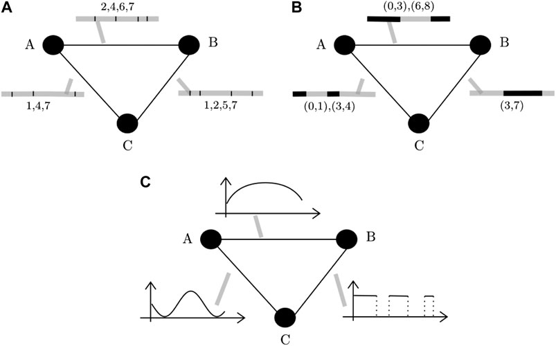
FIGURE 1. Types of temporal networks: The time of activation is indicated within the grey bar next to the edges (ranging between 0 and 8). For contact networks (A), edges activate only for one instant at the time and are marked with black vertical lines inside the grey bars. For example, in panel (A), the edge between nodes A and B is only active at instants 2, 4, 6, and 7. For interval networks (B), edges can be activated during an interval of time. For example, the edge between A and B in panel (B) is active during the time intervals (0, 3) and (6, 8). For contact networks (C), the edges are quantitatively more or less active across time, and the quantity of activity of any edge is described by a temporal function.

2.2 Flows and Trajectory Segments

We consider a function $\Phi :ℝ\times ℝ\times \Omega \to \Omega$, usually called flow on the spatial domain $\Omega$ of ${ℝ}^d$, satisfying the following properties:

$\{\begin{array}{l}\Phi \left(t,s,x\right)=\Phi \left(t,t^{\prime },\Phi \left(t\prime ,s,x\right)\right)\hfill \\ {\Phi }^{-1}(t,s,.)=\Phi (s,t,.),\hfill \end{array}(1)$

where $s,t,t^{\prime }\in ℝ$ and $x\in \Omega$. For fixed t and s, the flow $\Phi (t,s,\cdot )$ is a spatial transformation. For fixed x and varying s or t, the function gives a forward or backward trajectory of a particle over $\Omega$ between times $t\wedge s=\inf \left(t,s\right)$ and $t\vee s=\sup \left(t,s\right)$. If $s\le t$, $y=\Phi \left(t,s,x\right)$ gives the future location at time t of the particle presently located at x at time s. Contrarily, if $s\ge t$, $y=\Phi \left(t,s,x\right)$ gives the location at past time t that was occupied by the particle located at x at present time s. $\Phi (t,s,.)$ is assumed to be a bijective mapping meaning that particles following distinct trajectories cannot be at the same location at the same time.

In general, a flow is defined with respect to a possibly time-dependent vector field F over $ℝ\times \Omega$, as the solution $u:ℝ\to \Omega$ of an ordinary differential equation (see e.g., Hamilton’s equations in classical mechanics) with specified initial condition at a specified time s:

$\{\begin{array}{l}\frac{\text{d}u}{\text{d}t}\left(t\right)=F\left(t,u\left(t\right)\right)\hfill \\ u\left(s\right)=x,\hfill \end{array}(2)$

where F is continuous and Lipschitzian over $ℝ\times \Omega$. In the setting introduced above, $\Phi \left(t,s,x\right)=u\left(t\right)$ with $\Phi \left(s,s,x\right)$ = u(s) = x. The solution u represents the trajectory of the particle located at x at time s. Varying the initial condition in System (2), i.e. varying s and x, leads to consider pieces of trajectories of all particles which dynamics are governed by the vector field F. In this article, the vector field F will not be made explicit, but we will consider samples of trajectory segments (defined below) for constructing trajectory-based networks.

Definition 2.1. The trajectory segment associated to the flow $\Phi$ over the time interval ${\Delta }_{ts}=\left[t\wedge s,t\vee s\right]$, $s,t\in ℝ$, for a particle located at $x\in \Omega$ at time s is defined as follows:

$\Gamma \left(t,s,x\right)=\left\{\left(t^{\prime },\Phi \left(t^{\prime },s,x\right)\right):t^{\prime }\in {\Delta }_{ts}\right\}.(3)$

If $s<t$ (resp. $s>t$), $\Gamma \left(t,s,x\right)$ is a forward (resp. backward) trajectory segment. In this article, we are mainly interested in backward trajectories, but the framework presented here encompasses forward trajectories as well.

Example 2.1. The notions of flow and trajectory segment can be adapted to cope with air mass trajectories over the Earth surface. In this case, the spatial domain $\Omega$ representing the Earth surface is the sphere ${\mathcal{S}}^2$ in ${ℝ}^3$. If in addition, air masses are characterized by altitude and temperature evolving in space and time, then $\Omega ={\mathcal{S}}^2\times {ℝ}_{+}\times ℝ$, where ${ℝ}_{+}$ (resp. $ℝ$) is the domain of the altitude (resp. temperature) coordinate.

Example 2.2. Animal movements and behaviour activities can also be represented with the notions of flows and trajectory segments, providing, for instance, the animal locations and the covariate value indicating whether animals are feeding or not. In this case, $\Omega ={ℝ}^2\times \left\{\mathrm{0,1}\right\}$, where 1 stands for ‘the animal is feeding’ and 0 otherwise. The use of a binary variable for describing the feeding activity may require the use of stochastic processes or generalized functions undergoing dynamic analog to the System (2) for constructing the flow if it is defined with respect to a vector field F.

2.3 Pointwise and Integrated Connectivities

Trajectory-based networks are grounded on the notion of connectivity used as a quantitative, directed measurement of edges between graph nodes. In this aim, we first define the pointwise connectivity as a measure (or submeasure), in the mathematical sense, of the connectivity between a subset A and a point x of $\Omega$ induced by the trajectory segments $\Gamma \left(t,s,x\right)$ of a particle located at x at time s. Then, we use the pointwise connectivity to define the integrated connectivity between two subsets A and B of $\Omega$ over a temporal domain $\Delta$ of $ℝ$ ($\Delta$ can be the union of disjoint intervals).

Definition 2.2. Let $x\in \Omega$ and $A\in \mathrm{ℬ}\left(\Omega \right)$, where $\mathrm{ℬ}\left(\Omega \right)$ is a σ-algebra of subsets of $\Omega$. The pointwise connectivity associated to the flow $\text{Φ}$ is defined as a real valued function $\Psi$ on $\mathrm{ℬ}\left(\Omega \right)\times ℝ\times ℝ\times \Omega$, conveniently denoted by $\Psi \left(A|t,s,x\right)$, where $A\mapsto \Psi \left(A|t,s,x\right)$ is a measure or a submeasure on $\Omega$ for each $t,s,x$

Diverse types of the pointwise connectivity can be constructed, either using trajectory segments generated by $\Phi$, or directly using $\Phi$. Specific pointwise connectivities can include environmental covariates and even covariates associated to very the movements of particles. Below, we give several examples of such specifications. Some of these examples are graphically represented in Figure 2. Most examples are particularly relevant when $\Omega$ is a simple geographic domain and when $\Phi$ defines movements of individuals (e.g., air masses, animals or particles) within $\Omega$.

FIGURE 2

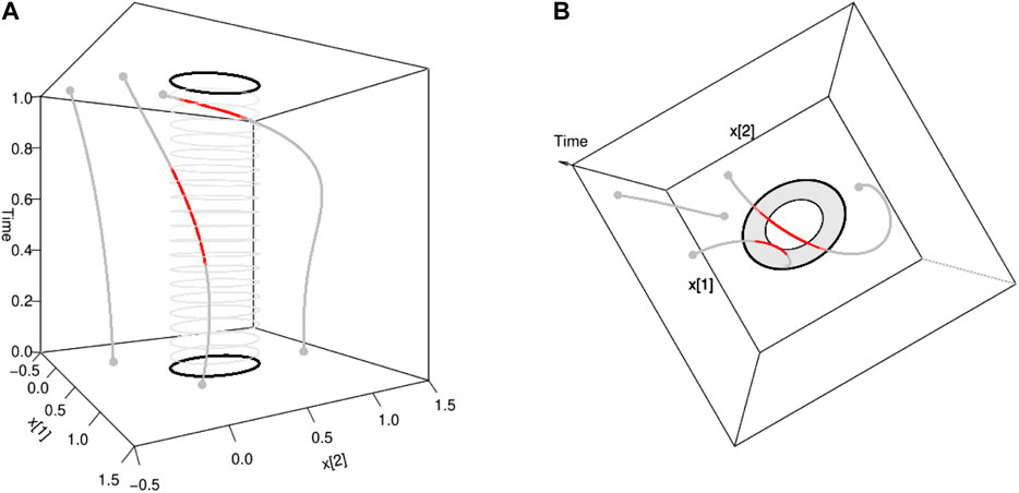
FIGURE 2. Illustration of contact-based, duration-based and length-based pointwise connectivities: ${\Psi }_C$, ${\Psi }_D$ and ${\Psi }_L$ are between the elliptic spatial domain $A\subset {ℝ}^2$ and different spatial points x at time $s=1$, for ${\Delta }_{ts}=\left[\mathrm{0,1}\right]$. The left curve on panel (A) never enters the domain A. The middle curve on panel (A) enters A (red part of the curve) over a relatively long duration [as shown by Panel (B)] but a short distance [as shown by Panel (B)]. The right curve on panel (A) enters A over a shorter duration but a longer distance. Thus, ${\Psi }_C\left(A|t,s,x\right)$, ${\Psi }_D\left(A|t,s,x\right)$ and ${\Psi }_L\left(A|t,s,x\right)$ are zero for the left curve; ${\Psi }_C\left(A|t,s,x\right)=1$ for the two other curves; ${\Psi }_D\left(A|t,s,x\right)$ is larger for the middle curve than for the right one, whereas ${\Psi }_L\left(A|t,s,x\right)$ is larger for the right curve than for the middle one.

Example 2.3. The contact-based pointwise connectivity is defined by:

${\Psi }_C\left(A|t,s,x\right)=1_{\{{\mathcal{A}}_{ts}{{\displaystyle \cap }}^{\text{Γ}}\Gamma (t,s,x)\ne \varnothing \}},(4)$

where ${\mathcal{A}}_{ts}={\Delta }_{ts}\times A$ and $1$ denotes the indicator function. ${\Psi }_C\left(A|t,s,x\right)$ indicates whether or not the particle whose movement in $\Omega$ is governed by $\Phi (\cdot ,s,x)$ hit A during the time interval ${\text{Δ}}_{ts}$. Note that $A\mapsto {\Psi }_C\left(A|t,s,x\right)$ is only a submeasure on $\Omega$ since ${\Psi }_C\left(A{{\displaystyle \cup }}^{\text{}}{A}^{\prime }|t,s,x\right)\le {\Psi }_C\left(A|t,s,x\right)+{\Psi }_C\left(A^{\prime }|t,s,x\right)$ for disjoint sets A and $A^{\prime }$ of $\mathrm{ℬ}\left(\Omega \right)$.

Remark 1. This example based on the simple contact between sets can be considered as too strict from a statistical and measure-theory perspective since the length or the duration of a contact may be null. Instead, a positive constraint on contact length for example can be used to define another version of the contact-based pointwise connectivity: Eq. 4 could then be replaced by

${\Psi }_{\tilde{C}}\left(A|t,s,x\right)=1_{\{\mathcal{L}\left({\mathcal{A}}_{ts}{{\displaystyle \cap }}^{\text{}}\Gamma (t,s,x)\right)>0\}},$

where $\mathcal{L}\left({\mathcal{A}}_{ts}{{\displaystyle \cap }}^{\text{}}\Gamma \left(t,s,x\right)\right)$ denotes the length of the curve $\text{Γ}$ within A. The length operator $\mathcal{L}$ will be made explicit in Example 2.5.

Example 2.4. The duration-based pointwise connectivity is defined by:

${\Psi }_D\left(A|t,s,x\right)=\underset{{\Delta }_{ts}}{{\displaystyle \int }}{1}_{\left\{\Phi \left(v,s,x\right)\in A\right\}}\text{d}v,(5)$

to measure the duration spent by the particle in A during ${\Delta }_{ts}$.

Example 2.5. The length-based pointwise connectivity is defined by:

${\Psi }_L\left(A|t,s,x\right)=\underset{{\Delta }_{ts}}{{\displaystyle \int }}{1}_{\left\{\Phi (v,s,x)\in A\right\}}\Vert D_v\Phi \left(v,s,x\right)\Vert \text{d}v,(6)$

where $D_v\Phi \left(v,s,x\right)$ stands for the derivative with respect to the time variable v of the flow $\Phi$ (which is a vector function), and $\left|\right|\cdot \left|\right|$ denotes the Euclidean norm. ${\Psi }_L\left(A|t,s,x\right)$ measures the distance travelled within A by the particle during ${\Delta }_{ts}$.

Example 2.6. The pointwise connectivity based on local volume is defined by:

${\Psi }_V\left(A|t,s,x\right)=\underset{{\Delta }_{ts}}{{\displaystyle \int }}{1}_{\left(\Phi \left(v,s,x\right)\in A\right)}\left|\det \left(J_{\Phi }^x\left(v,s\right)\right)\right|\text{d}v(7)$

where $\det \left(J_{\Phi }^x\left(v,s\right)\right)$ is the determinant of the Jacobian matrix (with respect to x) of the spatial transformation $\Phi (v,s,\cdot )$. The absolute value $\left|\det \left(J_{\Phi }^x\left(v,s\right)\right)\right|$ of the Jacobian determinant at x gives the ratio by which the function $\Phi (v,s,\cdot )$ expands/shrinks infinitesimal volumes around location x into infinitesimal volumes around location $\Phi \left(v,s,x\right)$. In other words, ${\Psi }_V\left(A|t,s,x\right)$ assesses how particle density increases or decreases from x to A along the time interval ${\Delta }_{ts}$. Intuitively, if n particles are initially in A and if the infinitesimal volume around any of these particles tends to shrink from A to x, then one expects a high concentration of particles in a fixed volume around x and, therefore, a high connectivity from A to x. Conversely, if the infinitesimal volume around a particle tends to expand from A to x, then one expects a lower concentration of particles in the same fixed volume around x and, therefore, a lower connectivity from A to x.

More sophisticated specifications of the pointwise connectivity can be proposed by incorporating spatio-temporal covariates in its formulation, like in the following examples.

Example 2.7. Let G denote a time-varying vector field defined over $ℝ\times \Omega$. The pointwise connectivity based on the external vector field G is defined by:

${\Psi }_G\left(A|t,s,x\right)=\underset{{\Delta }_{ts}}{{\displaystyle \int }}{1}_{\left(\Phi \left(v,s,x\right)\in A\right)}\left|<D_v\Phi \left(v,s,x\right),G\left(v,\Phi \left(v,s,x\right)\right)>\right|\text{d}v$

where $<D_v\Phi \left(v,s,x\right),G\left(v,\Phi \left(v,s,x\right)\right)>$ is the scalar product between the derivative with respect to the time variable v of the flow $\Phi$ (which is a vector function) and the vector field G. Larger the average collinearity in A between the instantaneous movement of the particle and the simultaneous direction of the vector field G, higher the connectivity between A and x. For instance, if $\Phi$ gives the movement of air masses and G provides the intensity and the direction of a continuous release of specific particles, then the connectivity will be high (resp. low) if the movement of the air in A and the movement of particles released in A are approximately collinear (resp. orthogonal).

Example 2.8. Let Z and $\tilde{Z}$ be positive real valued spatio-temporal functions defined over $ℝ\times \Omega$. The pointwise connectivity based on Z and $\tilde{Z}$ is defined by:

${\Psi }_{Z,\tilde{Z}}\left(A|t,s,x\right)=Z\left(s,x\right)\underset{{\Delta }_{ts}}{{\displaystyle \int }}{1}_{(\Phi (v,s,x)\in A)}\tilde{Z}\left(v,\Phi \left(v,s,x\right)\right)\text{d}v.(8)$

This form of pointwise connectivity may represent, for example, (i) the negative effect of the altitude of the air mass when it is above A on the recruitment of specific particles from the ground, and (ii) the positive effect of rainfall at $\left(s,x\right)$ on the deposition of particles from the air mass to the ground (see Figure 3). Thus, lower the average altitude of the air mass above A and more intense the rainfall at $\left(s,x\right)$, larger the contribution to the connectivity between A and x. This is expressed in Eq. 8 as follows: (i) $\tilde{Z}$ is defined as the binary function indicating whether or not the altitude of the air mass (located at x at time s) is lower than a threshold h when it is located at $\Phi \left(v,s,x\right)$ at time v; (ii) Z is a function of the local rainfall intensity at $\left(s,x\right)$.

FIGURE 3

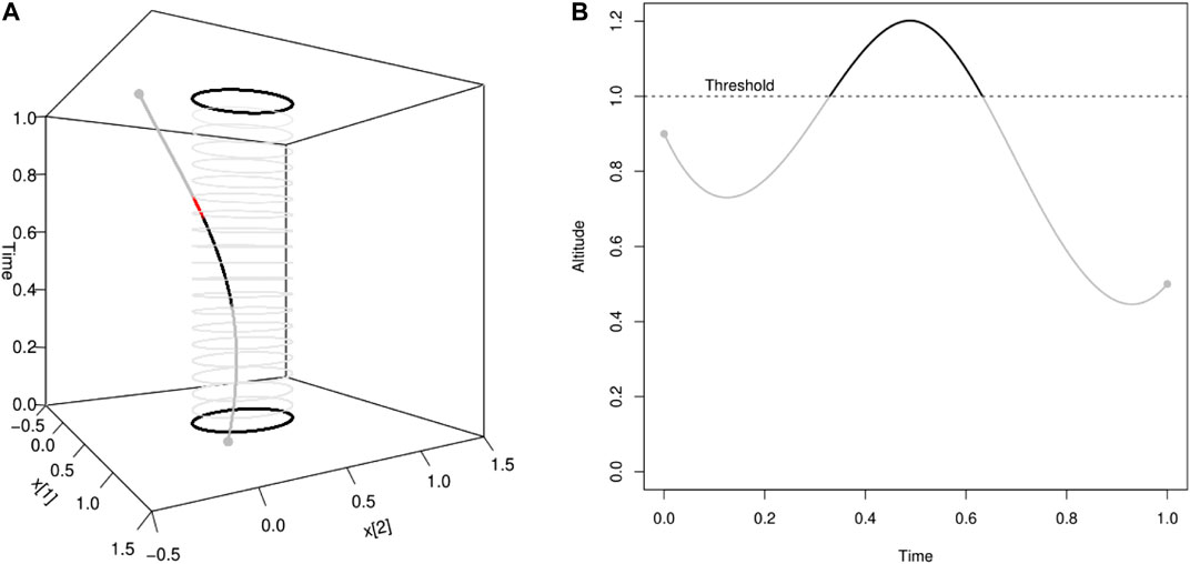
FIGURE 3. Illustration of pointwise connectivity based on a covariate measured along the trajectory: (see Example 2.8). In this illustration, the passage of the particle in the elliptic spatial domain A contributes to the pointwise connectivity [red part of the curve in Panel (A)] only when the particle is at an altitude lower than a threshold value [grey part of the curve in Panel (B)].

Remark 2. If in Example 2.8, the altitude of the air mass is incorporated as the third coordinate of $\Phi$ and A is a 3D-domain vertically limited by the threshold value h, then, Eq. 8 is simplify reduced to Eq. 5.

Remark 3. Example 2.8 could be generalized by considering a measure, say μ, over $ℝ$, to handle the potential contribution of discrete-time events to the pointwise connectivity:

${\Psi }_{Z,\mu }\left(A|t,s,x\right)=Z\left(s,x\right)\underset{{\Delta }_{ts}}{{\displaystyle \int }}{1}_{(\Phi (v,s,x)\in A)}\tilde{Z}\left(v,\Phi \left(v,s,x\right)\right)\text{d}\mu \left(v\right).(9)$

Remark 4. In the same vein, Example 2.8 can also be modified by adding within the integral the term $\Vert D_v\Phi \left(v,s,x\right)\Vert$ arising in Eq. 6 to account for a supplementary effect of the distance travelled within A on the pointwise connectivity.

Each pointwise connectivity defined above can be used for defining the integrated connectivity, which measures the quantitative directional link between two subsets A and B of $\mathrm{ℬ}\left(\Omega \right)$ generated by trajectories of particles located in B at times belonging to the temporal domain T.

Definition 2.3. Let A and B be two sets of $\mathrm{ℬ}\left(\Omega \right)$ and T a subset of the temporal domain $ℝ$. The δ-lag integrated connectivity linking B to A over T is defined by:

${\Psi }_{\nu ,\delta }^{\left(2\right)}\left(B\times A|T\right)=\underset{T\times B}{{\displaystyle \int }}\Psi \left(A|s+\delta ,s,x\right)\nu \left(\text{d}s,\text{d}x\right),(10)$

where $\delta \in ℝ$ and ν is a measure on $ℝ\times \Omega$.

Definition 2.3. encompasses connectivities generated by either forward or backward trajectories, depending on the sign of δ. The use of a unique duration $\left|\delta \right|$ could be relaxed to account for space-time heterogeneities in the duration of trajectories. It could even be infinite by introducing a measure over time like in Eq. 9.

The measure ν in Definition 2.3 can be continuous, discrete or hybrid over $ℝ\times \Omega \infty$. Indeed, if particles of interest are air masses, then B can be considered as continuously filled in space and time. Conversely, if particles of interest are animals of a specific species, then animals occupy only punctual locations in B at each time and the measure $x\mapsto \nu \left(\text{d}s,\text{d}x\right)$, given s, is discrete in $\Omega$, whereas the temporal component of ν is continuous. Another examples occurs when the time s corresponds to death times of animals, then ν is both discrete in space and time with a mass only at a countable collection of space-time points.

2.4 Trajectory–Based Network

Definition 2.4. A trajectory-based network generated by ${\Psi }_{\nu ,\delta }^{\left(2\right)}$ (given by Eq. 10) over the temporal domain $T\subset ℝ$, is a graph whose nodes $A_i,i=\left\{1,\dots ,I\right\}$, are disjoint sets of $\Omega$ in $\mathrm{ℬ}\left(\Omega \right)$ and whose directed edges are weighted by integrated connectivities $M_{ij}={\text{Ψ}}_{\nu ,\delta }^{\left(2\right)}\left(A_i\times A_j|T\right)$, $1\le i,j\le I$ and $i\ne j$.

Definition 2.4. corresponds to a spatial trajectory-based network evaluated over the fixed temporal domain T. It can be extended in different ways to obtain spatiotemporal analogs. For example, if $T_1,\dots ,T_K$ denote K disjoint but successive time intervals with equal lengths, then the sequence of trajectory-based networks generated by ${\Psi }_{\nu ,\delta }^{\left(2\right)}\left(\cdot \times \cdot |T_k\right)$, $k=1,\dots ,K$, forms a spatiotemporal trajectory-based network that can be analyzed to assess how connectivities across space are changing with time. This is one of the issues considered in Section 4.2.

3 Estimation of Integrated Connectivities

In practice, the integral defining the integrated connectivities between subsets of $\Omega$ (Definition 2.3) cannot be analytically computed in general, but can be estimated from a sample of trajectories. For instance, the integrated connectivity ${\Psi }_{\nu ,\delta }^{\left(2\right)}\left(B\times A|T\right)$ can be estimated by its empirical counterpart obtained by importance sampling, say ${\widehat{\Psi }}_{\nu ,\delta }^{\left(2\right)}\left(B\times A|T\right)$:

${\widehat{\Psi }}_{\nu ,\delta }^{\left(2\right)}\left(B\times A|T\right)=\frac{\left|T\right|}{N}\frac{\left|B\right|}{N^{\prime }}{\displaystyle \sum }_{k=1}^N{\displaystyle \sum }_{l=1}^{N^{\prime }}\Psi \left(A|s_k+\delta ,s_k,b_l\right),(11)$

where $s_1,\dots ,s_N\in T$ and $b_1,\dots ,b_{N\prime }\in B$ are times and locations, respectively, randomly drawn under the measure ν restricted to $T\times B$, $\left|T\right|$ and $\left|B\right|$ are the length and area of T and B, respectively, and $\Psi \left(A|s_k+\delta ,s_k,b_l\right)$ is the pointwise connectivity associated to the trajectory of the particle located at $b_l$ at time $s_k$ and observed over ${\Delta }_{s_k+\delta ,s_k}=\left[s_k\wedge s_k+\delta ,s_k\vee s_k+\delta \right]$.

If ν is constant, other classical numerical approaches can be applied to approximate the integral, such as an hybrid approach in which the mid-point rule is applied in time and a regular point process is used in space. In such a case, the integrated connectivity estimator is also given by Eq. 11.

Example 3.1. Using Eq. 11, the contact-based integrated connectivity corresponding to Example 2.3 is estimated by:

${\widehat{\Psi }}_{C,\delta }^{\left(2\right)}\left(B\times A|T\right)=\frac{\left|T\right|}{N}\frac{\left|B\right|}{N^{\prime }}{\displaystyle \sum }_{k=1}^N{\displaystyle \sum }_{l=1}^{N^{\prime }}{1}_{\left\{{\mathcal{A}}_{s_k+\delta ,s_k}{{\displaystyle \cap }}^{\text{}}\Gamma \left(s_k+\delta ,s_k,b_l\right)\ne \varnothing \right\}},(12)$

where ${\mathcal{A}}_{s_k+\delta ,s_k}={\Delta }_{s_k+\delta ,s_k}\times A$. Thus, ${\widehat{\Psi }}_{C,\delta }^{\left(2\right)}\left(B\times A|T\right)$ is simply the proportion of sampled trajectories intersecting A, multiplied by $\left|T\right|\left|B\right|$.

Example 3.2. Using Eq. 11, the duration-based integrated connectivity corresponding to Example 2.4 is estimated by the average duration of the intersections between the sampled trajectories and A, multiplied by $\left|T\right|\left|B\right|$.

Example 3.3 Using Eq. 11, the length-based integrated connectivity corresponding to Example 2.5 is estimated by the average length of the intersections between the sampled trajectories and A, multiplied by $\left|T\right|\left|B\right|$.

4 Applications

In this section, we applied our general framework to the flow of air mass movements. Indeed, these movements compiled over years were used to characterize climatic patterns [28] and to describe the transport of pollutants [29]. We show now how to deploy our approach for constructing air-mass movement networks in two real geographical contexts, namely the coastline of the Mediterranean Sea and the French region of Provence-Alpes-Côte d’Azur. These two examples have been chosen in order to prove the flexibility of our approach to different situations and geographical scales.

4.1 Case Study Regions and Network Construction

The first study region corresponds to the coast of the Mediterranean Sea, ranging approximately 1,600 km from north to south and 3,860 km from east to west. The temperate climate of the chosen region is strongly influenced by the presence of the Mediterranean Sea, with mild winters, hot summers and relatively scarce precipitations events. The landscape is characterized by coastal vegetation, typically shrubs and pines, and densely populated areas with intensive crop production of wheat, barley, vegetables and fruits, especially olive, grapes and citrus. In this paper, we characterize recurrent movements of air masses through the Mediterranean region by defining a grid with mesh size 74 km covering the coastline from 5 up to 250 km inland from the coast, including the four largest islands (namely Sicily, Sardinia, Cyprus and Corsica). Thus, we divide the region into 604 cells, where the centroids of the cells will be used as arrival locations of air-mass trajectories and will correspond to the nodes of the constructed network.

The second study region corresponds to the French region of Provence-Alpes-Côte d’Azur (PACA, hereafter), located in the south-eastern part of France and characterized by a rather complex landscape formed by a densely-populated coastline, agricultural lands (high-value-crops with fruit and olive orchards, vineyards, vegetable cultivation and horticulture), and natural mostly-alpines areas. The choice of this particular region is justified in the context of a research project aimed at assessing the potential long-distance dissemination of phytopathogenic bacterial populations that are known to be transported by air currents. The bacteria of interest (e.g., Pseudomonas syringae) can be lifted in to the air from a source location and then be passively transported by air masses until they are deposited back to land onto a different, far away sink location. Since the life cycles of the considered species of bacteria are strongly linked to the water cycle [30], we naturally partitioned the study area in a way that fit this assumption. Hence, we considered the 294 watersheds of the PACA region to define the sites that will later constitute the nodes of the constructed network. Since watersheds have irregular shapes and varying sizes, we selected a certain number of arrival locations per watershed (between 1 and 10 and proportionally to the watershed area) in order to cover the watersheds consistently according to the relative importance of their size and estimate the integrated connectivities. In total, a set of 833 arrival locations for air-mass trajectories was generated.

Once the arrival points for the two study regions have been established, we turned to the computation of air-mass trajectories arriving at the prescribed locations using the Hybrid Single-Particle Lagrangian Integrated Trajectory model (HYSPLIT [20]). The HYSPLIT model can be fed with meteorological data from the Global Data Assimilation System files with a 0.5-degree spatial resolution (GDAS) and was tuned by us to return 48 h backward air-mass trajectories arriving at the prescribed locations at an altitude of 500 m above mean sea level. A single trajectory consists of a vector containing the hourly positions (longitude, latitude and altitude) visited by the air mass before arriving at the specified location and time. Air-mass trajectories have been computed for every arrival location (604 for the Mediterranean region and 833 for the PACA region) and for every day between January 1, 2011 and December 31, 2017 (arrival hour is 12:00 GMT). The total number of computed trajectories is 1,543,220 for the Mediterranean region and 2,128,315 for the PACA region.

The final step for the construction of the networks is the estimation of the adjacency matrices of the networks, based on the methodology presented in the previous sections. To do that, for each pair of subsets of the spatial domain, we used the daily 48 h backward trajectories arriving at the locations sampled within the receptor subset, and computed the contact-based estimator (see Example 3.1). The subsets of the spatial domain are the watersheds for PACA and circular buffers of radius 20 km for the Mediterranean region, as in [8].

In this work we will consider networks corresponding to three temporal contexts: (i) the spatial networks obtained when T is the entire period 2011–2017, (ii) the yearly spatiotemporal networks formed by the seven spatial networks obtained when T₁ encompasses the year 2011, T₂ encompasses 2012 and so on, and (iii) monthly spatiotemporal networks formed by the twelve spatial networks obtained when T₁ represents every January from 2011 to 2017, T₂ every February from 2011 to 2017, and so on. In all these cases, we consider that the length of the time interval was one to easily compare the inferred networks (i.e., $\left|T\right|=1$ in Eqs. 11, 12).

4.2 Network Analysis

The networks we constructed are directed and weighted by contact-based connectivities generated by air mass trajectories and estimated with Eq. 12. They are inherently complex by the sheer amount of spatial and temporal information that they encompass. Hence, there is no easy way of representing the results either graphically or numerically, without compromising the original complexity of the networks. While a comprehensive study of the spatiotemporal properties of these networks goes beyond the scope of the paper, we explore some generic properties by means of well-known global topological indices:

• Density (Dens), is computed as the ratio between the sum of all edge weights and the number of all possible edges [31] and it measures how dense is a network with respect to a fully-connected network having the same number of nodes.

• Transitivity (Trans) or clustering, is computed by averaging the weighted clustering coefficient proposed by [25] across all nodes. This index measures the local cohesiveness of a node i with all the triples of its connected neighbors by considering their relative weights with respect to the node strength (defined as the sum of the weights of all the edges pointing to or from a node).

• Strength correlation (SC) is measured as the correlation between the incoming and outgoing strengths, computed as the sum of the weights of the edges pointing to or from a given node, respectively. Networks with positive (resp. negative) strength correlation are known to foster (resp. hamper) epidemic spread [32].

Other measures that are usually adopted to characterize network topology are meant to measure the length or cost associated to the movement between nodes following the edges of the network. We notice that, under the current framework, the weight computed between two nodes is proportional to the number of air-mass trajectories that connect them. Hence, higher values of the edge weight are associated to a higher connectivity between nodes. This is nonetheless incompatible with existing network search algorithms used to identify the shortest path between nodes since they usually consider the weight of an edge as a kind of distance or cost, hence the higher the weight, the less likely the connection between the nodes (e.g., the Dijkstra’s algorithm for weighted directed networks; ). On the other hand, it suffices to transform our weights into effective distances $d_{ij}=1-\log \left(w_{ij}\right)$ in order to obtain a representation of edge weights that is coherent with the distance interpretation of the search algorithms (), after having row standardized the adjacency matrices in order to ensure that $w_{ij}\in \left[\mathrm{0,1}\right],\forall i,j$. After this transformation, we then computed four more indices:

• the average shortest path between every pair of nodes, computed as the average shortest effective distance (ED);

• the average number of nodes in the shortest paths (ASP);

• the network diameter (Diam), computed as the maximum effective distance of a network, and the number of nodes that have to be crossed in this longest path;

• the small worldness (SW) property, computed as the ratio between the clustering and the average shortest path distance [33,34], that accounts for the facts that certain networks are highly clustered and have relatively short shortest paths, a condition that is known to favor rapid disease spread on the network.

4.3 Results

The two spatial trajectory-based networks representing the strength of tropospheric connections in the Mediterranean region and PACA during the entire period 2012 to 2017 are represented in Figure 4. It can be observed that the strongest connections tend to link nodes that are geographically close, but nonetheless moderate connections also exist between rather distant nodes (see also Supplementary Figure S1). The connectivity in PACA is mostly oriented from North-East to South-West, which corresponds to the direction of the prevailing wind in this region. For the Mediterranean basin, the orientation of the edges depends on the region and does not have a fixed direction (see Supplementary Figure S2). An interesting additional difference between the two networks is that the one for PACA has negative strength correlation (−0.85), meaning that nodes having a high incoming strength tend to have low outgoing degree, and vice versa. On the other hand, for the Mediterranean network, the value of the strength correlation is moderately positive (0.31), meaning that nodes having high incoming strength tend to have also high outgoing strength.

FIGURE 4

FIGURE 4. Networks weighted by contact-based connectivities generated by air mass trajectories: The connectivities are generated by air mass trajectories between (A) the 604 sampled circular areas within the Mediterranean basin and (B) the 294 watersheds of PACA. Edges with weights lower than 0.3 for (A) and $2\times {10}^3$ for (B) are not drawn. The cuts of the intervals in the two legends are chosen in such a way that each interval contains 20% of the observed data. The differences in the values taken by the connectivities in (A) and (B) are due to different measures of the area $\left|B\right|$ in Eqs. 11, 12: $\left|B\right|=1$ for each node in (A), whereas B is the actual area (expressed in km²) of each whatershed in (B).

Interestingly, we can observe that the indices provided in Tables 1,2 are overall more variable for the monthly spatiotemporal trajectory-based networks than for the yearly ones, indicating that the average air-mass connectivity is more variable within any given year than between different years. In order to confirm this observation, we performed a Ward-linkage hierarchical clustering method [35] based on the Euclidean distances of the standardized values of the 7 indices of Tables 1,2 for the monthly networks of the Mediterranean and PACA.

TABLE 1

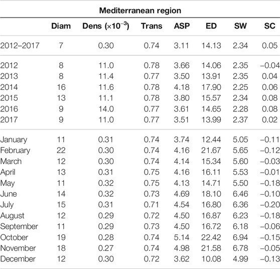
TABLE 1. Network indices [Diameter (Diam), density (Dens), transitivity (Trans), average shortest path (ASP), effective distance (ED), small worldness (SW), strength correlation (SC)] calculated from the networks covering the Mediterranean region and estimated in three temporal contexts: the entire period 2012–2017, yearly time periods from 2012 to 2017 and monthly time periods.

TABLE 2

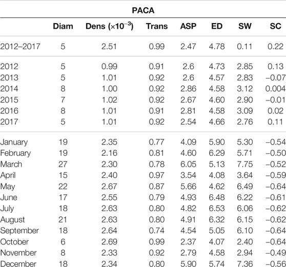
TABLE 2. Network indices [diameter (Diam), density (Dens), transitivity (Trans), average shortest path (ASP), effective distance (ED), small worldness (SW), strength correlation (SC)] calculated from the networks covering PACA and estimated in three temporal contexts: the entire period 2012–2017, yearly time periods from 2012 to 2017 and monthly time periods.

Figure 5A leads to the identification of three distinct seasons: summer (June, July, August, September), spring and winter (January, February, March, April, May and December) and fall (October, November). The spatial networks derived from the clustering are shown in Figures 5B–D, which display clear differences in the connectivity patterns: during spring and winter seasons, consistent and long-distance connections are observable along the Italian peninsula, moving from North to South, with sporadic connections on both sides towards Croatia and the western islands of Sardinia and Corsica. In the rest of the basin, connections tend to be local and with low or moderate intensity. During the summer season, the longest and most intense connections are observed in the western part of the basin (from Southern France and the Spanish southern coast to the north-western coast Africa). The network during the fall season correspond to intermediate situation between the above-mentionned networks. In terms of network indices (Figure 6A), it is clear that the winter air-mass connectivity network is more efficient than the summer one: it has higher density, transitivity and strength correlation, meaning that nodes are more frequently and strongly connected, while the longest path between every two nodes is shorter (lower diameter) and the average shortest path between nodes is lower, indicating that it is easier to move between any two given nodes of the network. These observations are particularly interesting if we consider the dissemination of airborne pathogens, that will be facilitated by winter connectivity regimes (irrespective of pathogens preference in terms of seasons).

FIGURE 5

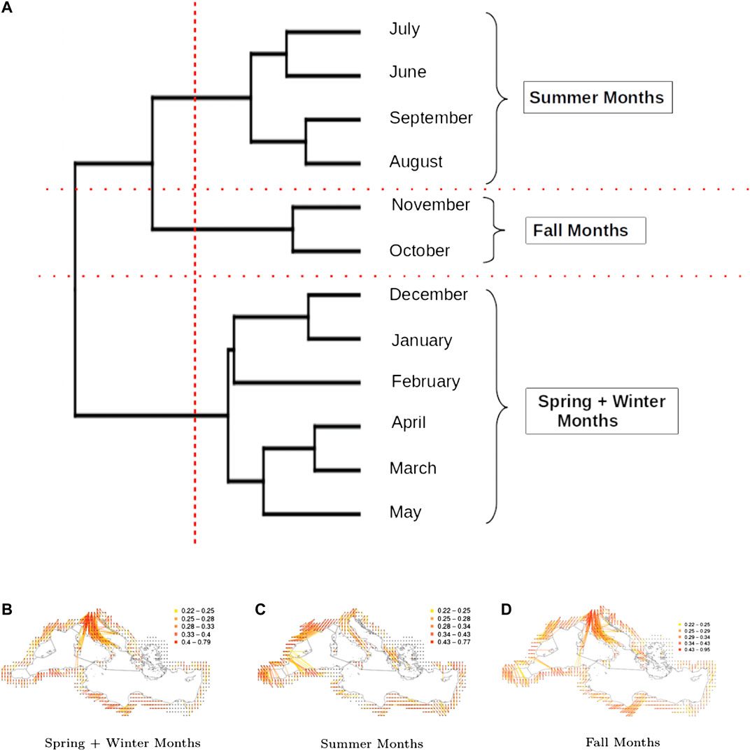
FIGURE 5. Clustering according to the indices calculated over the Mediterranean spatio-temporal network: (A): Dendrogram of the months obtained from a hierarchical cluster analysis of the Mediterranean spatio-temporal network based on the monthly dissimilarities of the indices presented in Table 1. (B), (C), and (D): Networks corresponding to the three identified clusters.

FIGURE 6

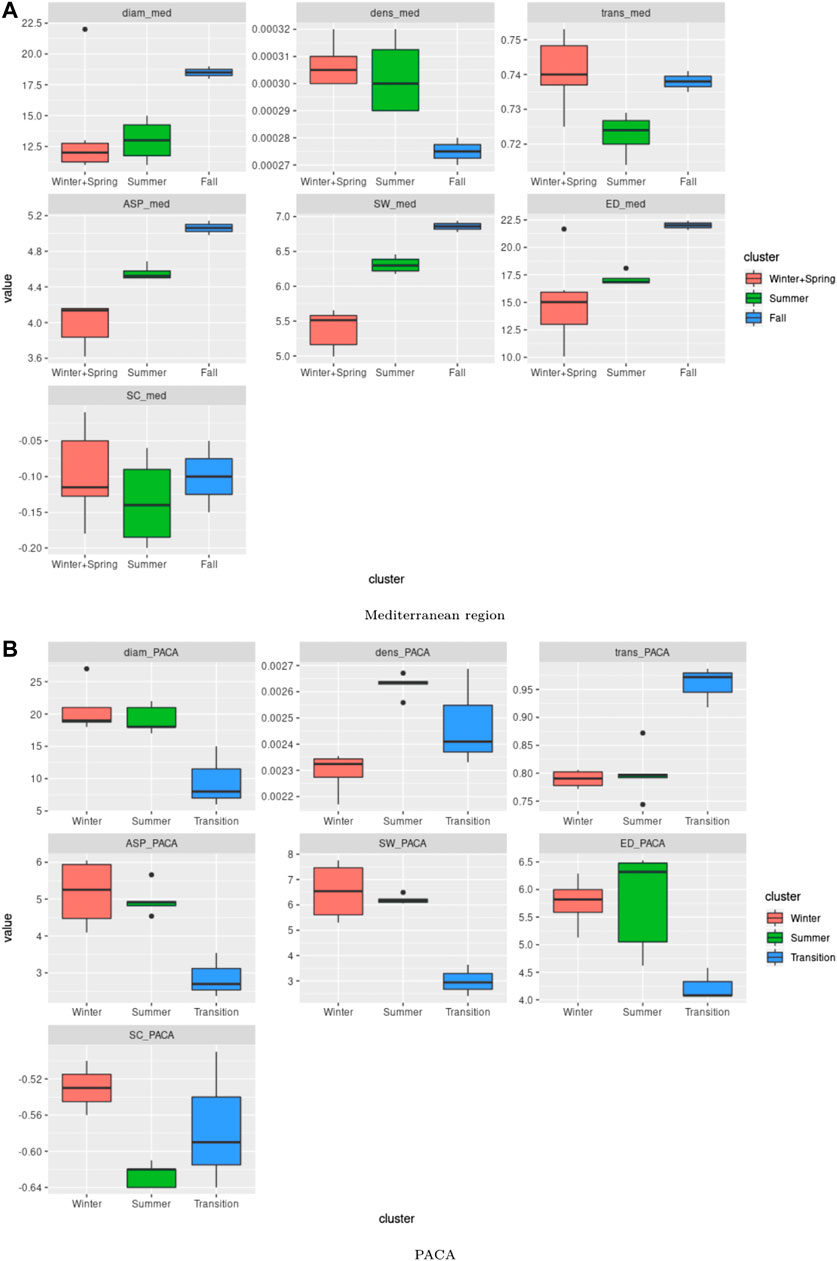
FIGURE 6. Boxplot for the computed indices over the Mediterranean and PACA regions: Boxplot for the different indices (Diameter, density, transitivity, average shortest path, small worldness, effective distance, strength correlation) obtained from (A) the two clusters identified for the Mediterranean region (see Figure 5) and (B) the three clusters for PACA (see Figure 7).

For the PACA region, the dendogram in Figure 7A allows us to identify three distinct clusters: winter (December, January, February, March), summer (May, June, July, August and September), and a set of transition months (April, October and November) separating the two above-mentionned seasons. Amongst the three clusters, the transition months stand out both in terms of network indices values (Figure 6B) and in terms of obtained spatial network (Figures 7B–D). In fact, it is characterized by the lowest diameter, average shortest path, small-worldness index and a strongly negative strength correlation, while it has the highest transitivity index and a rather high density. Compared to the two other clusters of networks, we observe that the networks of the transition months are more efficient in facilitating the flow between nodes and this can have interesting consequences when considering the possibility of airborne pathogen dispersion.

FIGURE 7

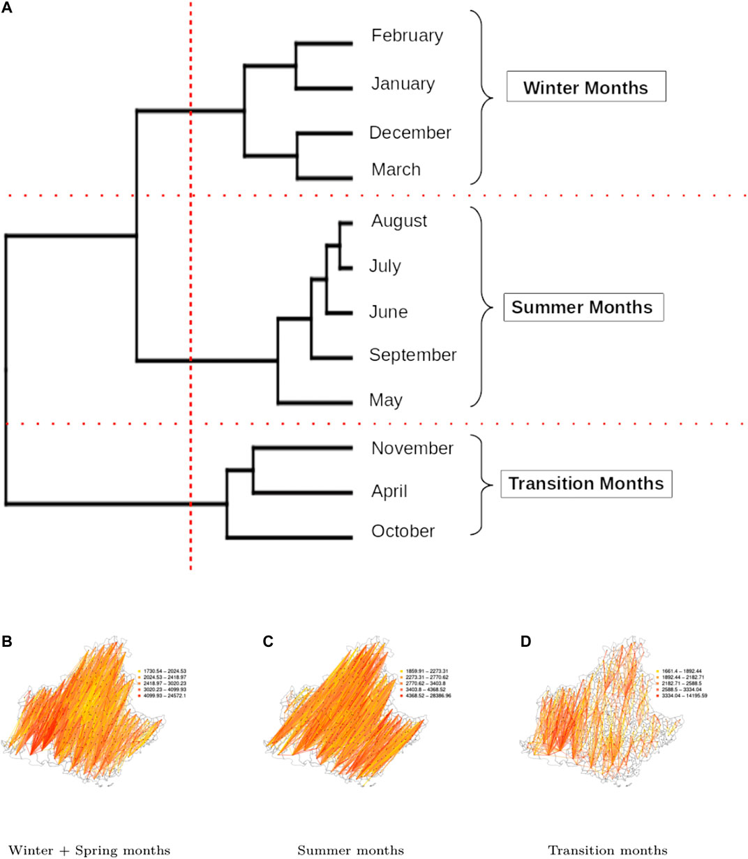
FIGURE 7. Clustering according to the indices calculated over the PACA spatio-temporal network: (A): Dendrogram of the months obtained from a hierarchical cluster analysis of the PACA spatio-temporal network based on the monthly dissimilarities of the indices presented in Table 2. (B), (C), and (D): Networks corresponding to the three identified clusters.

5 Discussion

We presented a framework for estimating and characterizing spatial and spatio-temporal networks generated by trajectory data. The development of this framework was motivated by the study of networks resulting from the movement of air masses sampled over long time periods and large spatial scales. Thus, in the application, we investigated the tropospheric connectivities across the Mediterranean basin and the French region PACA, and their variations through years and months. Our approach could be applied to diverse phenomena, from which trajectories can be observed. For instance, one could estimate networks generated by the movement of animals on the landscape scale based on animal trajectories observed with GPS devices [36]. This would allow the characterization of connectivity between different landscape components. Trajectories of human movement, transportation of specific goods (such as plant material) or trajectories of knowledge in social communities (that cannot be exhaustively observed) could also be used to estimate networks in other applied settings.

In Section 2.3, we proposed diverse measures of connectivity with different underlying (physical or biological) interpretations. Thus, the analyst can adapt the connectivity measure to the mechanistic processes he investigates, while we only considered the contact-based connectivity in our applications. Comparisons of contact-based, length-based and duration-based connectivities, not shown in this manuscript, led to little variations for the two case studies considered in this article. However, the use of covariates such as local rainfall and air-mass altitude for defining connectivities, as proposed in Section 2.3, is expected to impact the inferred networks and deserves to be explored. This perspective would be particularly relevant in the context of aerobiology: e.g., the airborne transport of organic particles, such as bacteria and fungal spores, that can be influenced by rainfall favoring the deposition of these particles [37].

In statistics, we are not only interested in point estimation, but also in the assessment of estimation uncertainties. In this paper, we however, focused on connectivity estimation, even if quantifying the estimation variance could have been useful for more rigorously investigating temporal variation in connectivities. Formally, the connectivity measures that we defined are integrals. Hence, results on integral numerical approximations (e.g., midpoint, trapezoidal or Monte Carlo integration) can be exploited to assess errors or variances of the connectivity estimates [38–40]. However, for this assessment, one should ideally consider dependencies between connectivity estimates for different pairs of nodes, which is not trivial. Further in-depth methodological developments are required to tackle this issue.

To more finely estimate connectivity, and its uncertainty, one could also take into account, if relevant, the uncertainty about the trajectories themselves. For example, when observed trajectories are smoothed versions of actual trajectories (as it is likely the case for air-mass trajectories calculated with HYSPLIT) or when the trajectories are partially observed and rather erratic, (i) a probabilistic model grounded on, for instance, a stochastic differential equation, could be used to reconstruct probable trajectories and (ii) the connectivity would be estimated from these reconstructed trajectories. Obviously, step (ii) should incorporate the uncertainty about the trajectory reconstruction impacted by an eventual preliminary step consisting in estimating the parameters of the above-mentioned probabilistic model.

Concerning the application treated in this article, we observed distinct seasonal (intra-annual) patterns in the temporal variation of the networks covering the Mediterranean coastline and PACA, whereas no evidence of inter-annual variation has been observed. In the case of the Mediterranean coastline, the networks corresponding to the three clusters shown in Figures 5B–D exhibit clearly distinct spatial patterns and, by looking at the variability of network indices in Figure 6A, we can observe that during winter the flow of air is more efficient in connecting distant parts of the region. In the case of PACA, we identified a third cluster that corresponds to transition months separating the spring-winter and summer seasons. Interestingly, these transition months show the highest connectivity. In the context of aerobiology, and more specifically regarding the diffusion of airborne plant pathogens, it is particularly important to identify the seasons where the spread of pathogen is more probable and to be able to represent the spatial connectivity during these periods.

In the long-term context of our applied research projects connected to aerobiology, the construction and exploration of networks generated by air-mass movements are a way to unravel epidemiological dynamics (and the resulting genetic patterns) of microbial pathogens disseminated at long distance via air movements in the troposphere (see [8]; for a proof of concept). Indeed, even if the pathogen is not explicitly taken into account by the framework proposed in this article, the description of connectivities that it offers provides us a proxy of airborne pathogen movements over long temporal terms and large spatial scales. This proxy is a mean to understand pathogen transportation and to anticipate its long distance dissemination. Specifically, network indices such as those calculated in this article can be associated with particular epidemiological properties such as the probability of long-distance transport of pathogens [41–43]. For instance, for plant pathogens, recent studies [44–46] showed that airborne populations of bacteria and fungi are rather constant across the years, while higher diversity can be observed in different seasons. This statement resonates with our analyses where we observed clear seasonal signals in the estimated monthly spatiotemporal networks in Section 4.3 whereas the yearly signals were less obvious.

Finally, the networks estimated using our approach could be a basis for developing epidemiological models (explicitly handling the pathogen) incorporating long-distance dissemination conditional on recurrent air-mass movements. Such models could be exploited to set up surveillance strategies for early warning and epidemic anticipation in order to help reduce the impacts of airborne pathogens on human health, agricultural production and ecosystem functioning [11].

Data Availability Statement

The datasets generated and analysed during the current study are available from the corresponding author on reasonable request.

Author Contributions

MC, DM, CEM, RS, SS contributed equally to this work. SS, RS and MC developed the theory; MC, DM, CEM and SS performed the applications. MC, DM and SS wrote the manuscript, RS and CEM reviewed it. All authors read and approved the final manuscript.

Funding

This research was funded by the SPREE project from the French National Research Agency (Grant No. ANR–17–CE32–0004–01) and the PHYTOSENTINEL project (Grant No. IB–2019–SPE).

Conflict of Interest

The authors declare that the research was conducted in the absence of any commercial or financial relationships that could be construed as a potential conflict of interest.

Acknowledgments

The authors thank Loïc Houde for his technical assistance in the calculation of trajectories with HYSPLIT. This article has been released as a pre-print at arxiv, [47].

Supplementary Material

The Supplementary Material for this article can be found online at: https://www.frontiersin.org/articles/10.3389/fams.2020.602621/full#supplementary-material.

References

1. Mahura, AG, Korsholm, US, Baklanov, AA, and Rasmussen, A. Elevated birch pollen episodes in Denmark: contributions from remote sources. Aerobiologia (2007). 23:171. doi:10.1007/s10453-007-9061-3

CrossRef Full Text | Google Scholar

2. Šauliene, I, and Veriankaite, L. Application of backward air mass trajectory analysis in evaluating airborne pollen dispersion. J Environ Eng Landsc Manag (2006). 14:113–120.

Google Scholar

3. Bogawski, P, Borycka, K, Grewling, Ł, and Kasprzyk, I. Detecting distant sources of airborne pollen for Poland: Integrating back-trajectory and dispersion modelling with a satellite-based phenology. Sci Total Environ (2019). 689:109–125. doi:10.1016/j.scitotenv.2019.06.348

PubMed Abstract | CrossRef Full Text | Google Scholar

4. Khaniabadi, YO, Daryanoosh, SM, Amrane, A, Polosa, R, Hopke, PK, Goudarzi, G, et al. Impact of Middle Eastern Dust storms on human health. Atmos Pollut Res (2017). 8:606–613. doi:10.1016/j.apr.2016.11.005

CrossRef Full Text | Google Scholar

5. Aciego, S, Riebe, C, Hart, S, Blakowski, M, Carey, C, Aarons, S, et al. Dust outpaces bedrock in nutrient supply to montane forest ecosystems. Nat Commun (2017). 8:14800. doi:10.1038/ncomms14800

PubMed Abstract | CrossRef Full Text | Google Scholar

6. Moroz, BE, Beck, HL, Bouville, A, and Simon, SL. Predictions of dispersion and deposition of fallout from nuclear testing using the NOAA-HYSPLIT meteorological model. Health Phys (2010). 99:252–269. doi:10.1097/hp.0b013e3181b43697

PubMed Abstract | CrossRef Full Text | Google Scholar

7. Rolph, G, Ngan, F, and Draxler, R. Modeling the fallout from stabilized nuclear clouds using the HYSPLIT atmospheric dispersion model. J Environ Radioact (2014). 136:41–55. doi:10.1016/j.jenvrad.2014.05.006

PubMed Abstract | CrossRef Full Text | Google Scholar

8. Leyronas, C, Morris, CE, Choufany, M, and Soubeyrand, S. Assessing the aerial interconnectivity of distant reservoirs of sclerotinia sclerotiorum. Front Microbiol (2018). 9:2257. doi:10.3389/fmicb.2018.02257

PubMed Abstract | CrossRef Full Text | Google Scholar

9. Wang, H, Yang, X, and Ma, Z. Long-distance spore transport of wheat stripe rust pathogen from Sichuan, Yunnan, and Guizhou in southwestern China. Plant Disease (2010). 94:873–880. doi:10.1094/pdis-94-7-0873

PubMed Abstract | CrossRef Full Text | Google Scholar

10. Aylor, DE. The role of intermittent wind in the dispersal of fungal pathogens. Annu Rev Phytopathol (1990). 28:73–92. doi:10.1146/annurev.py.28.090190.000445

CrossRef Full Text | Google Scholar

11. Mundt, CC, Sackett, KE, Wallace, LD, Cowger, C, and Dudley, JP. Aerial dispersal and multiple-scale spread of epidemic disease. EcoHealth (2009). 6:546–552. doi:10.1007/s10393-009-0251-z

PubMed Abstract | CrossRef Full Text | Google Scholar

12. Sadyś, M, Skjøth, CA, and Kennedy, R. Back-trajectories show export of airborne fungal spores (Ganoderma sp.) from forests to agricultural and urban areas in England. Atmos Environ (2014). 84:88–99. doi:10.1016/j.atmosenv.2013.11.015

CrossRef Full Text | Google Scholar

13. Hiraoka, S, Miyahara, M, Fujii, K, Machiyama, A, and Iwasaki, W. Seasonal analysis of microbial communities in precipitation in the greater Tokyo area Japan. Front Microbiol (2017). 8:1506. doi:10.3389/fmicb.2017.01506

PubMed Abstract | CrossRef Full Text | Google Scholar

14. Liu, T, Marlier, ME, DeFries, RS, Westervelt, DM, Xia, KR, Fiore, AM, et al. Seasonal impact of regional outdoor biomass burning on air pollution in three Indian cities: Delhi, Bengaluru, and Pune. Atmos Environ (2018b). 172:83–92. doi:10.1016/j.atmosenv.2017.10.024

CrossRef Full Text | Google Scholar

15. Liu, B, Ma, Y, Gong, W, Zhang, M, and Yang, J. Study of continuous air pollution in winter over Wuhan based on ground-based and satellite observations. Atmos Pollut Res (2018a). 9:156–165. doi:10.1016/j.apr.2017.08.004

CrossRef Full Text | Google Scholar

16. Talbi, A, Kerchich, Y, Kerbachi, R, and Boughedaoui, M. Assessment of annual air pollution levels with PM1, PM2.5, PM10 and associated heavy metals in Algiers, Algeria. Environ Pollut (2018). 232:252–263. doi:10.1016/j.envpol.2017.09.041

PubMed Abstract | CrossRef Full Text | Google Scholar

17. Chen, Y, and Luo, Y. Analysis of paths and sources of moisture for the South China rainfall during the presummer rainy season of 1979–2014. J Meteorol Res (2018). 32:744–757. doi:10.1007/s13351-018-8069-7

CrossRef Full Text | Google Scholar

18. Armon, M, Dente, E, Smith, JA, Enzel, Y, and Morin, E. Synoptic-scale control over modern rainfall and flood patterns in the levant drylands with implications for past climates. J Hydrometeorol (2018). 19:1077–1096. doi:10.1175/jhm-d-18-0013.1

CrossRef Full Text | Google Scholar

19. Rabinowitz, JL, Lupo, AR, Market, PS, and Guinan, PE. An investigation of atmospheric rivers impacting heavy rainfall events in the North-Central Mississippi River Valley. Int J Climatol (2019). 39:4091–4106. doi:10.1002/joc.6061

CrossRef Full Text | Google Scholar

20. Stein, A, Draxler, RR, Rolph, GD, Stunder, BJ, Cohen, M, and Ngan, F. NOAA’s HYSPLIT atmospheric transport and dispersion modeling system. Bull Amer Meteor Soc (2015). 96:2059–2077. doi:10.1175/bams-d-14-00110.1

CrossRef Full Text | Google Scholar

21. Margosian, ML, Garrett, KA, Hutchinson, JS, and With, KA. Connectivity of the American agricultural landscape: assessing the national risk of crop pest and disease spread. BioScience (2009). 59:141–151. doi:10.1525/bio.2009.59.2.7

CrossRef Full Text | Google Scholar

22. Newman, ME. The structure and function of complex networks. SIAM Rev (2003). 45:167–256. doi:10.1137/s003614450342480

CrossRef Full Text | Google Scholar

23. Strogatz, SH. Exploring complex networks. Nature (2001). 410:268. doi:10.1038/35065725

PubMed Abstract | CrossRef Full Text | Google Scholar

24. West, DB, et al. Introduction to graph theory. 2nd ed. Upper Saddle River, NJ: Prentice Hall (1996).

25. Barrat, A, Barthelemy, M, Pastor-Satorras, R, and Vespignani, A. The architecture of complex weighted networks. PNAS (2004). 101:3747–3752. doi:10.1073/pnas.0400087101

PubMed Abstract | CrossRef Full Text | Google Scholar

26. Barthélemy, M. Spatial Networks. New York, United States: Springer (2014).

27. Holme, P, and Saramäki, J. Temporal networks. Phys Rep (2012). 519:97–125. doi:10.1016/j.physrep.2012.03.001

CrossRef Full Text | Google Scholar

28. Hondula, DM, Sitka, L, Davis, RE, Knight, DB, Gawtry, SD, Deaton, ML, et al. A back-trajectory and air mass climatology for the Northern Shenandoah Valley, USA. Int J Climatol (2010). 30:569–581. doi:10.1002/joc.1896

CrossRef Full Text | Google Scholar

29. Pérez, IA, Artuso, F, Mahmud, M, Kulshrestha, U, Sánchez, ML, and García, M. Applications of air mass trajectories. Adv Meteorol (2015). 2015:20. doi:10.1155/2015/284213

CrossRef Full Text | Google Scholar

30. Morris, CE, Sands, DC, Vinatzer, BA, Glaux, C, Guilbaud, C, Buffiere, A, et al. The life history of the plant pathogen Pseudomonas syringae is linked to the water cycle. ISME J (2008). 2:321. doi:10.1038/ismej.2007.113

PubMed Abstract | CrossRef Full Text | Google Scholar

31. Liu, G, Wong, L, and Chua, HN. Complex discovery from weighted ppi networks. Bioinformatics (2009). 25:1891–1897. doi:10.1093/bioinformatics/btp311

PubMed Abstract | CrossRef Full Text | Google Scholar

32. Pautasso, M, Xu, X, Jeger, MJ, Harwood, TD, Moslonka-Lefebvre, M, and Pellis, L. Disease spread in small-size directed trade networks: the role of hierarchical categories. J Appl Ecol (2010). 47:1300–1309. doi:10.1111/j.1365-2664.2010.01884.x

CrossRef Full Text | Google Scholar

33. Li, W, Lin, Y, and Liu, Y. The structure of weighted small-world networks. Physica A (2007). 376:708–718. doi:10.1016/j.physa.2006.10.015

CrossRef Full Text | Google Scholar

34. Colon-Perez, LM, Couret, M, Triplett, W, Price, CC, and Mareci, TH. Small worldness in dense and weighted connectomes. Front Phys (2016). 4:14. doi:10.3389/fphy.2016.00014

PubMed Abstract | CrossRef Full Text | Google Scholar

35. Ferreira, L, and Hitchcock, DB. A comparison of hierarchical methods for clustering functional data. Commun Stat Simul Comput (2009). 38:1925–1949. doi:10.1080/03610910903168603

CrossRef Full Text | Google Scholar

36. Bastille-Rousseau, G, Douglas-Hamilton, I, Blake, S, Northrup, JM, and Wittemyer, G. Applying network theory to animal movements to identify properties of landscape space use. Ecol Appl (2018). 28:854–864. doi:10.1002/eap.1697

PubMed Abstract | CrossRef Full Text | Google Scholar

37. Morris, CE, Soubeyrand, S, Bigg, EK, Creamean, JM, and Sands, DC. Mapping rainfall feedback to reveal the potential sensitivity of precipitation to biological aerosols. Bull Amer Meteor Soc (2017). 98:1109–1118. doi:10.1175/bams-d-15-00293.1

CrossRef Full Text | Google Scholar

38. Davis, PJ, and Rabinowitz, P. Methods of numerical integration. 2nd ed. Chelmsford, United States: Courier Corporation (2007).

39. Caflisch, RE. Monte carlo and quasi-monte carlo methods. Acta Numer (1998). 7:1–49. doi:10.1017/s0962492900002804

CrossRef Full Text | Google Scholar

40. Geweke, J. Monte carlo simulation and numerical integration. Handbook Comput Econ (1996). 1:731–800. doi:10.1016/s1574-0021(96)01017-9

CrossRef Full Text | Google Scholar

41. Moslonka-Lefebvre, M, Finley, A, Dorigatti, I, Dehnen-Schmutz, K, Harwood, T, Jeger, MJ, et al. Networks in plant epidemiology: from genes to landscapes, countries, and continents. Phytopathology (2011). 101:392–403. doi:10.1094/phyto-07-10-0192

PubMed Abstract | CrossRef Full Text | Google Scholar

42. Jeger, MJ, Pautasso, M, Holdenrieder, O, and Shaw, MW. Modelling disease spread and control in networks: implications for plant sciences. New Phytol (2007). 174:279–297. doi:10.1111/j.1469-8137.2007.02028.x

PubMed Abstract | CrossRef Full Text | Google Scholar

43. Pautasso, M, and Jeger, MJ. Network epidemiology and plant trade networks. AoB Plants (2014). 6. doi:10.1093/aobpla/plu007

PubMed Abstract | CrossRef Full Text | Google Scholar

44. Nicolaisen, M, West, JS, Sapkota, R, Canning, GG, Schoen, C, and Justesen, AF. Fungal communities including plant pathogens in near surface air are similar across Northwestern Europe. Front Microbiol (2017). 8:1729. doi:10.3389/fmicb.2017.01729

PubMed Abstract | CrossRef Full Text | Google Scholar

45. Bowers, RM, Clements, N, Emerson, JB, Wiedinmyer, C, Hannigan, MP, and Fierer, N. Seasonal variability in bacterial and fungal diversity of the near-surface atmosphere. Environ Sci Technol (2013). 47:12097–12106. doi:10.1021/es402970s

PubMed Abstract | CrossRef Full Text | Google Scholar

46. Aho, K, Weber, C, Christner, B, Vinatzer, B, Morris, C, Joyce, R, et al. Spatiotemporal patterns of microbial composition and diversity in precipitation. Ecol Monogr (2019). 90:e01394. doi:10.1002/ecm.1394

CrossRef Full Text | Google Scholar

47. Choufany, M, Martinetti, D, Senoussi, R, Morris, CE, and Soubeyrand, S. Spatiotemporal large-scale networks shaped by air mass movements (2019). [arXiv preprint arXiv:1911.07007].

Google Scholar