Statistical Analysis of Multi-Relational Network Recovery

In this paper, we develop asymptotic theories for a class of latent variable models for large-scale multi-relational networks. In particular, we establish consistency results and asymptotic error bounds for the (penalized) maximum likelihood estimators when the size of the network tends to infinity. The basic technique is to develop a non-asymptotic error bound for the maximum likelihood estimators through large deviations analysis of random fields. We also show that these estimators are nearly optimal in terms of minimax risk.

1. Introduction

A multi-relational network (MRN) describes multiple relations among a set of entities simultaneously. Our work on MRNs is mainly motivated by its applications to knowledge bases that are repositories of information. Examples of knowledge bases include WordNet [1], Unified Medical Language System [2], and Google Knowledge Graph (https://developers.google.com/knowledge-graph). They have been used as the information source in many natural language processing tasks, such as word-sense disambiguation and machine translation [3–5]. A knowledge base often includes knowledge on a large number of real-world objects or concepts. When a knowledge base is characterized by MRN, the objects and concepts correspond to nodes, and knowledge types are relations. Figure 1 provides an excerpt from an MRN in which “Earth,” “Sun,” and “solar system” are three nodes. The knowledge about the orbiting patterns of celestial objects forms a relation “orbit,” and the knowledge on classification of the objects forms another relation “belong to” in the MRN.

FIGURE 1

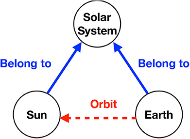
Figure 1. An example of the MRN representation of a knowledge base.

An important task of network analysis is to recover the unobserved network based on data. In this paper, we consider a latent variable model for MRNs. The presence of an edge from node i to node j of relation type k is a Bernoulli random variable Y_ijk with success probability M_ijk. Each node is associated with a vector, θ, called the embedding of the node. The probability M_ijk is modeled as a function f of the embeddings, θ_i and θ_j, and a relation-specific parameter vector w_k. This is a natural generalization of the latent space model for single-relational networks [6]. Recently, it has been successfully applied to knowledge base analysis [7–14]. Various forms of f are proposed, such as distance models [7], bilinear models [12–14], and neural networks [15]. Computational algorithms are proposed to improve link prediction for knowledge bases [16, 17]. The statistical properties of the embedding-based MRN models have not been rigorously studied. It remains unknown whether and to what extent the underlying distribution of MRN can be recovered, especially when there are a large number of nodes and relations.

The results in this paper fill in the void by studying the error bounds and asymptotic behaviors of the estimators for M_ijk's for a general class of models. This is a challenging problem due to the following facts. Traditional statistical inference of latent variable models often requires a (proper or improper) prior distribution for θ_i. In such settings, one works with the marginalized likelihood with θ_i integrated out. For the analysis of MRN, the sample size and the latent dimensions are often so large that the above-mentioned inference approaches are computationally infeasible. For instance, a small-scale MRN could have a sample size as large as a few million, and the dimension of the embeddings is as large as several hundred. Therefore, in practice, the prior distribution is often dropped, and the latent variables θ_i's are considered as additional parameters and estimated via maximizing the likelihood or penalized likelihood functions. The parameter space is thus substantially enlarged due to the addition of θ_i's whose dimension is proportionate to the number of entities. As a result, in the asymptotic analysis, we face a double-asymptotic regime of both the sample size and the parameter dimension.

In this paper, we develop results for the (penalized) maximum likelihood estimator of such models and show that under regularity conditions the estimator is consistent. In particular, we overcome the difficulty induced by the double-asymptotic regime via non-asymptotic bounds for the error probabilities. Then, we show that the distribution of MRN can be consistently estimated in terms of average Kullback-Leibler (KL) divergence even when the latent dimension increases slowly as the sample size tends to infinity. A probability error bound is also provided together with the upper bound for the risk (expected KL divergence). We further study the lower bound and show the near-optimality of the estimator in terms of minimax risk. Besides the average KL divergence, similar results can be established for other criteria, such as link prediction accuracy.

The outline of the remaining sections is as follows. In section 2, we provide the model specification and formulate the problem. Our main results are presented in section 3. Finite sample performance is examined in section 4 through simulated and real data examples. Concluding remarks are included in section 5.

2. Problem Setup

2.1. Notation

Let | · | be the cardinality of a set and × be the Cartesian product. Set {1, …, N} is denoted by [N]. The sign function sgn(x) is defined to be 1 for x ≥ 0 and 0 otherwise. The logistic function is denoted by σ(x) = e^x/(1 + e^x). Let 1_A be the indicator function on event A. We use U[a, b] to denote the uniform distribution on [a, b] and Ber(p) to denote the Bernoulli distribution with probability p. The KL divergence between Ber(p) and Ber(q) is written as $D(p\left|\right|q)=plog\frac{p}{q}+(1-p)log\frac{1-p}{1-q}$. We use || · || to denote the Euclidean norm for vectors and the Frobenius norm for matrices.

For two real positive sequences {a_n} and {b_n}, we write a_n = O(b_n) if lim sup_n→∞ a_n/b_n < ∞. Similarly, we write a_n = Ω(b_n) if lim sup_n→∞ b_n/a_n < ∞ and a_n = o(b_n) if $\underset{n\to \infty }{lim}{\mathit{a}}_n/b_n=0$. We denote a_n ≲ b_n if lim sup_n→∞ a_n/b_n ≤ 1. When {a_n} and {b_n} are negative sequences, a_n ≲ b_n means liminf_n→∞ a_n/b_n ≥ 1. In some places, we use b_n ≳ a_n as an interchangeable notation of a_n ≲ b_n. Finally, if $\underset{n\to \infty }{lim}{\mathit{a}}_n/b_n=1$, we write a_n ~ b_n.

2.2. Model

Consider an MRN with N entities and K relations. Given i, j ∈ [N] and k ∈ [K], the triple λ = (i, j, k) corresponds to the edge from entity i to entity j of relation k. Let Λ = [N] × [N] × [K] denote the set of all edges. We assume in this paper that an edge can be either present or absent in a network and use Y_λ ∈ {0, 1} to indicate the presence of edge λ. In some scenarios, the status of an edge may have more than two types. Our analysis can be generalized to accommodate these cases.

We associate each entity i with a vector θ_i of dimension d_E and each relation k with a vector w_k of dimension d_R. Let ${E}\subseteq {ℝ}^{d_E}$ be a compact domain where the embeddings θ₁, …, θ_N live. We call ${R}$ the entity space. Similarly, we define a compact relation space ${R}\subseteq {ℝ}^{d_R}$ for the relation-specific parameters w₁, …, w_K. Let x = (θ₁, …, θ_N, w₁, …, w_K) be a vector in the product space Θ = ${E}$^N × ${R}$^K. The parameters associated with edge λ = (i, j, k) is then x_λ = (θ_i, θ_j, w_k). We assume that given x, elements in {Y_λ ∣ λ ∈ Λ} are independent with each other and that the log odds of Y_λ = 1 is

$\begin{array}{ll}log\frac{P(Y_{\lambda }=1|x)}{P(Y_{\lambda }=0|x)}=\varphi (x_{\lambda }),\text{for }\lambda \in \Lambda .& (1)\end{array}$

Here ϕ is defined on ${E}$² × ${R}$, and ϕ(x_λ) is often called the score of edge λ.

We will use Y to represent the N × N × K tensor formed by {Y_λ ∣ λ ∈ Λ} and M(x) to represent the corresponding probability tensor {P(Y_λ = 1 ∣ x) ∣ λ ∈ Λ}. Our model is given by

$\begin{array}{ll}{Y}_{\lambda }~\text{Ber}\left(M_{\lambda }\left(x^{*}\right)\right),& (2)\end{array}$

$\begin{array}{ll}{M}_{\lambda }(x)=\sigma (\varphi (x_{\lambda })),\lambda \in \Lambda ,& (3)\end{array}$

where x^* stands for the true value of x and Y_λ's are independent. In the above model, the probability of the presence of an edge is entirely determined by the embeddings of the corresponding entities and the relation-specific parameters. This imposes a low-dimensional latent structure on the probability tensor M^* = M(x^*).

We specify our model using a generic function ϕ. It includes various existing models as special cases. Below are two examples of ϕ.

1. Distance model [7].

$\begin{array}{ll}\varphi ({\theta }_i,{\theta }_j,w_k)=b_k-||{\theta }_i+a_k-{\theta }_j{||}^2,& (4)\end{array}$

where ${\theta }_i,{\theta }_j,{\mathit{a}}_k\in {ℝ}^d$, b_k ∈ ℝ and w_k = (a_k, b_k). In the distance model, relation k from node i to node j is more likely to exist if θ_i shifted by a_k is closer to θ_j under the Euclidean norm.

2. Bilinear model [9].

$\begin{array}{ll}\varphi ({\theta }_i,{\theta }_j,w_k)={\theta }_i^{T}diag(w_k){\theta }_j,& (5)\end{array}$

where ${\theta }_i,{\theta }_j,{\mathit{w}}_k\in {ℝ}^d$ and diag(w_k) is a diagonal matrix with w_k as the diagonal elements. Model (5) is a special case of the more general model $\varphi ({\theta }_i,{\theta }_j,{\mathit{w}}_k)={\theta }_i^T{\mathit{w}}_k{\theta }_j$, where $W_k\in {ℝ}^{d\times d}$ is a matrix parameterized by ${\mathit{w}}_k\in {ℝ}^{d_R}$. Trouillon et al. [12], Nickel et al. [13], and Liu et al. [14] explored different ways of constructing w_k.

Very often, only a small portion of the network is observed [18]. We assume that each edge in the MRN is observed independently with probability γ and that the observation of an edge is independent of Y. Let ${S}$ ⊂ Λ be the set of observed edges. Then the elements in ${S}$ are independent draws from Λ. For convenience, we use n to represent the expected number of observed edges, namely, n = E[|${S}$|] = γ|Λ| = γN²K. Our goal is to recover the underlying probability tensor M^* based on the observed edges {Y_λ ∣ λ ∈ ${S}$}.

REMARK 1. Ideally, if there exists x^* such that $Y_{\lambda }=\mathrm{\text{sgn}}(M_{\lambda }({\mathit{x}}^{*})-\frac{1}{2})$ for all λ ∈ Λ, then Y can be recovered with no error under x^*. This is, however, a rare case in practice, especially for large-scale MRN. A relaxed assumption is that Y can be recovered with some low dimensional x^* and noise {ϵ_λ} such that

$\begin{array}{ll}{Y}_{\lambda }=\text{sgn}\left(M_{\lambda }(x^{*})+{ϵ}_{\lambda }-\frac{1}{2}\right),{ϵ}_{\lambda }\stackrel{i.i.d}{~}U\left[-\frac{1}{2},\frac{1}{2}\right],\forall \lambda \in \Lambda .& (6)\end{array}$

By introducing the noise term, we formulate the deterministic MRN as a random graph. The model described in (2) is an equivalent but simpler form of (6).

2.3. Estimation

According to (2), the log-likelihood function of our model is

$\begin{array}{ll}l(x;Y_{{S}})={\displaystyle \sum _{\lambda \in {S}}}{Y}_{\lambda }log{M}_{\lambda }(x)+(1-Y_{\lambda })log(1-M_{\lambda }(x)).& (7)\end{array}$

We omit the terms $\sum _{\lambda \in {S}}log\gamma +\sum _{\lambda \notin {S}}log(1-\gamma )$ in (7) since γ is not the parameter of interest. To obtain an estimator of M^*, we take the following steps.

1. Obtain the maximum likelihood estimator (MLE) of x^*,

$\begin{array}{ll}\widehat{x}={\displaystyle \underset{x\in \Theta }{argmax}}l(x;Y_{{S}}).& (8)\end{array}$

2. Use the plug-in estimator

$\begin{array}{ll}\widehat{M}=M(\widehat{x})& (9)\end{array}$

as an estimator of M^*.

In (8), the estimator $\widehat{\mathit{x}}$ is a maximizer over the compact parameter space Θ = ${E}$^N × ${R}$^K. The dimension of Θ is

$m=N{d}_E+K{d}_R,$

which grows linearly in the number of entities N and the number of relations K.

2.4. Evaluation Criteria

We consider the following criteria to measure the error of the above-mentioned estimator. They will be used in both the main results and numerical studies.

1. Average KL divergence of the predictive distribution from the true distribution

$\begin{array}{ll}L(\widehat{M},M^{*})=\frac{1}{|\Lambda |}{\displaystyle \sum _{\lambda \in \Lambda }}D(M_{\lambda }^{*}||{\widehat{M}}_{\lambda }).& (10)\end{array}$

2. Mean squared error of the predicted scores

$\begin{array}{ll}MS{E}_{\varphi }=\frac{1}{|\Lambda |}{\displaystyle \sum _{\lambda \in \Lambda }}{(\varphi ({\widehat{x}}_{\lambda })-\varphi (x_{\lambda }^{*}))}^2.& (11)\end{array}$

3. Link prediction error

$\begin{array}{ll}\widehat{err}=\frac{1}{|\Lambda |}{\displaystyle \sum _{\lambda \in \Lambda }}{1}_{{Ŷ}_{\lambda }\ne Y_{\lambda }^{*}},& (12)\end{array}$

where ${Ŷ}_{\lambda }=\mathrm{\text{sgn }}\left({\widehat{M}}_{\lambda }-\frac{1}{2}\right)$ and $Y_{\lambda }^{*}=\mathrm{\text{sgn }}\left(M_{\lambda }^{*}-\frac{1}{2}\right)$.

REMARK 2. The latent attributes of entities and relations are often not identifiable, so the MLE $\widehat{\mathit{x}}$ is not unique. For instance, in (4), the values of ϕ and M(x) remain the same if we replace θ_i and a_k, respectively by Γθ_i + t and Γa_k, where t is an arbitrary vector in ${ℝ}^{d_E}$ and Γ is an orthonormal matrix. Therefore, we consider the mean squared error of scores, which are identifiable.

3. Main Results

We first provide results of the MLE in terms of KL divergence between the estimated and the true model. Specifically, we investigate the tail probability $P(L(\widehat{M},M^{*})>t)$ and the expected loss $E[L(\widehat{M},M^{*})]$. In section 3.1, we discuss upper bounds for the two quantities. The lower bounds are provided in section 3.2. In section 3.3, we extend the results to penalized maximum likelihood estimators (pMLE) and other loss functions. All proofs are included in the Supplementary Materials.

3.1. Upper Bounds

We first present an upper bound for the tail probability $P(L(\widehat{M},M^{*})>t)$ in Lemma 1. The result depends on the tensor size, the number of observed edges, the functional form of ϕ, and the geometry of parameter space Θ. The lemma explicitly quantifies the impact of these element on the error probability. It is key to the subsequent analyses. Lemma 2 gives a non-asymptotic upper bound for the expected loss (risk). We then establish the consistency of $\widehat{M}$ and the asymptotic error bounds in Theorem 1.

We will make the following assumptions throughout this section.

ASSUMPTION 1. x^* ∈ Θ = ${E}$^N × ${R}$^K, where ${E}$ and ${R}$ are Euclidean balls of radius U.

ASSUMPTION 2. The function ϕ is Lipschitz continuous under the Euclidean norm,

$\begin{array}{ll}|\varphi (u)-\varphi (v)|\le \alpha ||u-v||,\forall u,v\in {{E}}^2\times {R},& (13)\end{array}$

where α is a Lipschitz constant.

Assumption 1 is imposed for technical convenience. The results can be easily extended to general compact parameter spaces. Let $C=\underset{u\in {{E}}^2\times {R}}{sup}\left|\varphi (u)\right|$. Without loss of generality, we assume that C ≥ 2.

LEMMA 1. Consider $\widehat{M}$ defined in (9) and the average KL divergence L in (10). Under Assumptions 1 and 2, for every t > 0, β > 0 and 0 < s < nt,

$\begin{array}{r}{\displaystyle P\left(L\left(\widehat{M},M^{*}\right)\ge t\right)\le exp\left\{-\frac{nt-s}{C}h\left(\frac{1}{2}-\frac{s}{2nt}\right)\right\}}\\ {\displaystyle {\left(1+\frac{2\sqrt{3}\alpha Un\left(1+\beta \right)}{s}\right)}^m+exp\left\{-n\beta h\left(\beta \right)\right\},}& (14)\end{array}$

where m = Nd_E + Kd_R is the dimension of Θ, n = γN²K is the expected number of observations, and $h(u)=(1+\frac{1}{u})log(1+u)-1$.

In the proof of Lemma 1, we use Bennett's inequality to develop a uniform bound that does not depend on the true parameters. It is sufficient for the current analysis. If the readers need sharper bounds, they can read through the proof and replace the Bennett's bound by the usual large deviation rate function which provides a sharp exponential bound that depends on the true parameters. We don't pursue this direction in this paper.

Lemma 2 below gives an upper bound of risk $E[L(\widehat{M},M^{*})]$, which follows from Lemma 1.

LEMMA 2. Consider $\widehat{M}$ defined in (9) and loss function L in (10). Let C₁ = 18C, $C_2=8\sqrt{3}\alpha U$ and C₃ = 2 max {C₁, C₂}. If Assumptions 1 and 2 hold and $\frac{n}{m}\ge C_2+e$, then

$\begin{array}{r}E\left[L(\widehat{M},M^{*})\right]\le C_3\frac{m}{n}log\frac{n}{m}+\frac{C_1}{n}exp\left\{-mlog\frac{n}{m}\right\}\\ +\frac{3}{n}exp\left\{-\frac{1}{3}\left(n+C_{3}mlog\frac{n}{m}\right)\right\}.& (15)\end{array}$

We are interested in the asymptotic behavior of the tail probability in two scenarios: (i) t is a fixed constant and (ii) t decays to zero as the number of entities N tends to infinity. The following theorem gives an asymptotic upper bound for the tail probability and the risk.

THEOREM 1. Consider $\widehat{M}$ defined in (9) and the loss function L in (10). Let the number of entities N → ∞ and C, K, U, d_E, d_R, α, and γ be fixed constants. If Assumptions 1 and 2 hold, we have the following asymptotic inequalities.

When t is a fixed constant,

$\begin{array}{ll}logP(L(\widehat{M},M^{*})\ge t)\lesssim -\frac{t}{5C}n.& (16)\end{array}$

When $t=10C\frac{m}{n}log\frac{n}{m}$,

$\begin{array}{ll}logP(L(\widehat{M},M^{*})\ge t)\lesssim -mlog\frac{n}{m}.& (17)\end{array}$

Furthermore,

$\begin{array}{ll}E[L(\widehat{M},M^{*})]\lesssim 10C\frac{m}{n}log\frac{n}{m}.& (18)\end{array}$

The consistency of $\widehat{M}$ is implied by (16) and the rate of convergence is $|logP(L(\widehat{M},M^{*})\ge t)|=\Omega (N^2)$ if t is a fixed constant. The rate decreases to Ω(N log N) for the choice of t producing (17). It is also implied by (17) that $L(\widehat{M},M^{*})=O(\frac{1}{N}logN)$ with high probability. We show in the next section that this upper bound is reasonably sharp.

The condition that K, U, d_E, d_R, and α are fixed constants can be relaxed. For instance, we can let U, d_E, d_R, and α go to infinity slowly at the rate O(log N) and K at the rate O(N). We can let γ go to zero provided that $\frac{m}{n}log\frac{n}{m}=o(1)$.

3.2. Lower Bounds

We show in Theorem 2 that the order of the minimax risk is $\Omega (\frac{m}{n})$, which implies the near optimality of $\widehat{M}$ in (9) and the upper bound $O(\frac{m}{n}log\frac{n}{m})$ in Theorem 1. To begin with, we introduce the following definition and assumption.

DEFINITION 1. For u = (θ, θ′, w) ∈ ${E}$² × ${R}$, the r-neighborhood of u is

$\begin{array}{r}{{N}}_r(u)=\{(\eta ,{\eta }^{\prime },\zeta )\in {{E}}^2\times {R}\mid ||\eta -\theta ||\le r,||{\eta }^{\prime }-{\theta }^{\prime }||\le r,||\zeta \\ -w||\le r\}.\end{array}$

Similarly, for $\mathit{x}=({\mathit{\theta }}_1,\dots ,{\mathit{\theta }}_N,{\mathit{w}}_1,\dots ,{\mathit{w}}_K)\in {{E}}^N\times {{R}}^K$, the r-neighborhood of x is

$\begin{array}{r}{{N}}_r(x)=\{({\eta }_1,\dots ,{\eta }_N,{\zeta }_1,\dots ,{\zeta }_K)\in {{E}}^N\times {{R}}^K\mid ||{\eta }_i-{\theta }_i||\le r,||\\ {\zeta }_k-w_k||\le r,\forall i\in \left[N\right],k\in \left[K\right]\}.\end{array}$

ASSUMPTION 3. There exists $u_0\in {{E}}^2\times {R}$ and r, κ > 0 such that ${{N}}_r(u_0)\subset {{E}}^2\times {R}$ and

$\begin{array}{ll}|\sigma (\varphi (u))-\sigma (\varphi (v))|\ge \kappa ||u-v||,\forall u,v\in {{N}}_r(u_0).& (19)\end{array}$

THEOREM 2. Let $b={sup}_{u\in {{N}}_r(u_0)}\sigma (\varphi (u))$. Under Assumptions 2 and 3, if $r^2\ge \frac{(m/16-1)b(1-b)}{12{\alpha }^{2}n}$, then for any estimator $\widehat{M}$, there exists x^* ∈ Θ such that

$\begin{array}{ll}{\displaystyle P\left(L\left(\widehat{M},M^{*}\right)>\tilde{C}\frac{m/16-1}{n}\right)\ge \frac{1}{2},}& (20)\end{array}$

where $\tilde{C}=\frac{{\kappa }^{2}b(1-b)}{108{\alpha }^2}$. Consequently, the minimax risk

$\begin{array}{ll}{\displaystyle \underset{\widehat{M}}{min}}{\displaystyle \underset{M^{*}}{max}}E[L(\widehat{M},M^{*})]\ge \tilde{C}\frac{m/16-1}{2n}.& (21)\end{array}$

3.3. Extensions

3.3.1. Reguralization

In this section, we extend our asymptotic results in Theorem 1 to regularized estimators. In practice, regularization is often considered to prevent overfitting. We consider a regularization similar to elastic net [19]

$\begin{array}{ll}{l}_{\rho }(x;Y_{{S}})=l(x;Y_{{S}})-{\rho }_1||x{||}_1-{\rho }_2||x{||}^2,& (22)\end{array}$

where || · ||₁ stands for L₁ norm and ρ₁, ρ₂ ≥ 0 are regularization parameters. The pMLE is

$\begin{array}{ll}\widehat{x}=argma{x}_{x\in \Theta }{l}_{\rho }(x;Y_{{S}}).& (23)\end{array}$

Note that the MLE in (8) is a special case of the pMLE above with ρ₁ = ρ₂ = 0. Since $\widehat{\mathit{x}}$ is shrunk toward 0, without loss of generality, we assume that ${E}$ and ${R}$ are centered at 0. We generalize Theorem 1 to pMLE in the following theorem.

THEOREM 3. Consider the estimator $\widehat{M}$ given by (23) and (9) and the loss function L in (10). Let the number of entities N → ∞ and C, K, U, d_E, d_R, α, γ be absolute constants. If Assumptions 1 and 2 hold and ρ₁ + ρ₂ = o(log N), then asymptotic inequalities (16), (17), and (18) in Theorem 1 hold.

3.3.2. Other Loss Functions

We present some results for the mean squared error loss MSE_ϕ defined in (11) and the link prediction error $\widehat{err}$ defined in (12). Corollaries 1 and 2 give upper and lower bounds for MSE_ϕ, and Corollary 3 gives an upper bound for $\widehat{err}$ under an additional assumption.

COROLLARY 1. Under the setting of Theorem 3 with the loss function replaced by MSE_ϕ, we have the following asymptotic results.

If t is a fixed constant,

$\begin{array}{ll}logP(MS{E}_{\varphi }\ge t)\lesssim -\frac{5\sigma (C)(1-\sigma (C))t}{2C}n.& (24)\end{array}$

If $t=\frac{20C}{\sigma (C)(1-\sigma (C))}\frac{m}{n}log\frac{n}{m}$,

$\begin{array}{ll}logP(MS{E}_{\varphi }\ge t)\lesssim -mlog\frac{n}{m}.& (25)\end{array}$

Furthermore,

$\begin{array}{ll}E\left[MS{E}_{\varphi }\right]\lesssim \frac{20C}{\sigma (C)(1-\sigma (C))}\frac{m}{n}log\frac{n}{m}.& (26)\end{array}$

COROLLARY 2. Under the setting of Theorem 2 with the loss function replaced by MSE_ϕ, we have

$\begin{array}{ll}{\displaystyle P\left(MS{E}_{\varphi }>\tilde{C}\frac{m/16-1}{8n}\right)\ge \frac{1}{2},}& (27)\end{array}$

and

$\begin{array}{ll}{\displaystyle \underset{\widehat{M}}{min}}{\displaystyle \underset{M^{*}}{max}}E\left[MS{E}_{\varphi }\right]\ge \tilde{C}\frac{m/16-1}{16n}.& (28)\end{array}$

ASSUMPTION 4. There exists ε > 0 such that $\left|M_{\lambda }^{*}-\frac{1}{2}\right|\ge \epsilon$ for every λ ∈ Λ.

COROLLARY 3. Under the setting of Theorem 3 with the loss function replaced by $\widehat{err}$ and Assumption 4 added, we have the following asymptotic results.

If t is a fixed constant,

$\begin{array}{ll}logP(\widehat{err}\ge t)\lesssim -\frac{2{\epsilon }^{2}t}{5C}n.& (29)\end{array}$

If $t=\frac{5C}{{\epsilon }^2}\frac{m}{n}log\frac{n}{m}$,

$\begin{array}{ll}logP(\widehat{err}\ge t)\lesssim -mlog\frac{n}{m}.& (30)\end{array}$

Furthermore,

$\begin{array}{ll}E\left[\widehat{err}\right]\lesssim \frac{5C}{{\epsilon }^2}\frac{m}{n}log\frac{n}{m}.& (31)\end{array}$

3.3.3. Sparse Representations

We are interested in sparse entity embeddings and relation parameters. Let || · ||₀ be the number of non-zero elements of a vector and τ be a pre-specified sparsity level of x (i.e., the proportion of non-zero elements). Let m_τ = mτ be the upper bound of non-zero parameters, that is, $\left|\right|{\mathit{x}}^{*}|{|}_0\le m_{\tau }$. Consider the following estimator

$\begin{array}{ll}\widehat{x}={\displaystyle \underset{x\in \Theta }{argmax}}l(x;Y_{{S}})\text{subject to\hspace{1em}}||x{||}_0\le m_{\tau }.& (32)\end{array}$

The estimator defined above maximizes the L₀-penalized log-likelihood.

THEOREM 4. Consider $\widehat{M}$ defined in (32) and (9) and the loss function L in (10). Let the number of entities N → ∞ and τ, C, K, U, d_E, d_R, α be absolute constants. Under Assumptions 1 and 2, the following asymptotic inequalities hold.

If t is a fixed constant,

$\begin{array}{ll}logP(L(\widehat{M},M^{*})\ge t)\lesssim -\frac{t}{5C}n.& (33)\end{array}$

If $t=10C\frac{m_{\tau }}{n}log\frac{n}{m_{\tau }}$,

$\begin{array}{ll}logP(L(\widehat{M},M^{*})\ge t)\lesssim -m_{\tau }log\frac{n}{m_{\tau }}.& (34)\end{array}$

Furthermore,

$\begin{array}{ll}E[L(\widehat{M},M^{*})]\lesssim 10C\frac{m_{\tau }}{n}log\frac{n}{m_{\tau }}.& (35)\end{array}$

We omit the results for other loss functions as well as the lower bounds since they can be analogously obtained.

4. Numerical Examples

In this section, we demonstrate the finite sample performance of $\widehat{M}$ through simulated and real data examples. Throughout the numerical experiments, AdaGrad algorithm [20] is used to compute $\widehat{\mathit{x}}$ in (8) or (23). It is a first-order optimization method that combines stochastic gradient descent (SGD) [21] with adaptive step sizes for finding the local optima. Since the objective function in (8) is non-convex, a global maximizer is not guaranteed. Our objective function usually has many global maximizers, but, empirically, we found the algorithm works well on MRN recovery and the recovery performance is insensitive to the choice of the starting point of SGD. Computationally, SGD is also more appealing to handle large-scale MRNs than those more expensive global optimization methods.

4.1. Simulated Examples

In the simulated examples, we fix K = 20, d = 20 and consider various choices of N ranging from 100 to 10,000 to investigate the estimation performance as N grows. The function ϕ we consider is a combination of the distance model (4) and the bilinear model (5),

$\begin{array}{ll}\varphi ({\theta }_i,{\theta }_j,w_k)={({\theta }_i+a_k-{\theta }_j)}^{T}diag(b_k)({\theta }_i+a_k-{\theta }_j),& (36)\end{array}$

where ${\mathit{\theta }}_i,{\mathit{\theta }}_j,{\mathit{a}}_k,{\mathit{b}}_k\in {ℝ}^d$ and w_k = (a_k, b_k). We independently generate the elements of ${\mathit{\theta }}_i^{*}$, ${\mathit{a}}_k^{*}$, and ${\mathit{b}}_k^{*}$ from normal distributions N(0, 1), N(0, 1), and N(0, 0.25), respectively, where N(μ, σ²) denotes the normal distribution with mean μ and variance σ². To guarantee that the parameters are from a compact set, the normal distributions are truncated to the interval [−20, 20]. Given the latent attributes, each Y_ijk is generated from the Bernoulli distribution with success probability $M_{ijk}^{*}=\sigma (\varphi ({\mathit{\theta }}_i^{*},{\mathit{\theta }}_j^{*},{\mathit{w}}_k^{*}))$. The observation probability γ takes value from {0.005, 0.01, 0.02}. For each combination of γ and N, 100 independent datasets are generated. For each dataset, we compute $\widehat{\mathit{x}}$ and $\widehat{M}$ in (8) and (9) with AdaGrad algorithm and then calculate $L(\widehat{M},M^{*})$ defined in (10) as well as the link prediction error $\widehat{err}$ defined in (12). The two types of losses are averaged over the 100 datasets for each combination of N and γ to approximate the theoretical risks $E[L(\widehat{M},M^{*})]$ and $E[\widehat{err}]$. These quantities are plotted against N in log scale in Figure 2. As the figure shows, in general, both risks decrease as N increases. When N is small, n/m is not large enough to satisfy the condition n/m ≥ C₂ + e in Lemma 2 and the expected KL risk increases at the beginning. After N gets sufficiently large, the trend agrees with our asymptotic analysis.

FIGURE 2

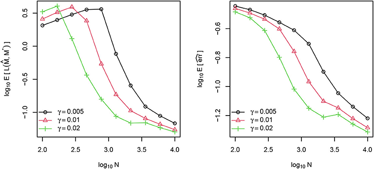
Figure 2. Average Kullback-Leibler divergence (left) and average link prediction error (right) of $\widehat{M}$ for different choices of N and γ.

4.2. Real Data Example: Knowledge Base Completion

WordNet [1] is a large lexical knowledge base for English. It has been used in word sense disambiguation, text classification, question answering, and many other tasks in natural language processing [3, 5]. The basic components of WordNet are groups of words. Each group, called a synset, describes a distinct concept. In WordNet, synsets are linked by conceptual-semantic and lexical relations, such as super-subordinate relation and antonym. We model WordNet as an MRN with the synsets as entities and the links between synsets as relations.

Following Bordes et al. [7], we use a subset of WordNet for analysis. The dataset contains 40,943 synsets and 18 types of relations. A triple (i, j, k) is called valid if relation k from entity i to entity j exists, i.e., Y_ijk = 1. All the other triples are called invalid triples. Among more than 3.0 × 10¹⁰ possible triples in WordNet, only 151,442 triples are valid. We assume that 141,442 valid triples and the same proportion of invalid triples are observed. The goal of our analysis is to recover the unobserved part of the knowledge base. We adopt the ranking procedure, which is commonly used in knowledge graph embedding literature, to evaluate link predictions. Given a valid triple λ = (i, j, k), we rank estimated scores for all the invalid triples inside ${\Lambda }_{·jk}=\left\{(i^{\prime },j,k)\mid i^{\prime }\in [N]\right\}$ in descending order and call the rank of $\varphi ({\widehat{\mathit{x}}}_{\lambda })$ as the head rank of λ, denoted by H_λ. Similarly, we can define the tail rank T_λ and the relation rank R_λ by ranking $\varphi ({\widehat{\mathit{x}}}_{\lambda })$ among the estimated scores of invalid triples in Λ_ij· and Λ_i·k, respectively. For a set V of valid triples, the prediction performance can be evaluated by rank-based criteria, mean rank (MR), mean reciprocal rank (MRR), and hits at q (Hits@q), which are defined as

${\text{MR}}_{\text{E}}=\frac{1}{2\left|V\right|}{\displaystyle \sum _{\lambda \in V}}{H}_{\lambda }+T_{\lambda },{\text{MR}}_{\text{R}}=\frac{1}{\left|V\right|}{\displaystyle \sum _{\lambda \in V}}{R}_{\lambda },$

${\text{MRR}}_{\text{E}}=\frac{1}{2\left|V\right|}{\displaystyle \sum _{\lambda \in V}}\frac{1}{H_{\lambda }}+\frac{1}{T_{\lambda }},{\text{MRR}}_{\text{R}}=\frac{1}{\left|V\right|}{\displaystyle \sum _{\lambda \in V}}\frac{1}{R_{\lambda }},$

and

${\text{Hits}}_{\text{E}}@q=\frac{1}{2\left|V\right|}{\displaystyle \sum _{\lambda \in V}}{1}_{\left\{H_{\lambda }\le q\right\}}+1_{\left\{T_{\lambda }\le q\right\}},$

${\text{Hits}}_{\text{R}}@q=\frac{1}{\left|V\right|}{\displaystyle \sum _{\lambda \in V}}{1}_{\left\{R_{\lambda }\le q\right\}}.$

The subscripts E and R represent the criteria for predicting entities and relations, respectively. Models with higher MRRs, Hits@q's or lower MRs are more preferable. In addition, MRR is more robust to outliers than MR.

The three models described in (4), (5), and (36) are considered in our data analysis and we refer to them as Model 1, 2, and 3, respectively. For each model, the latent dimension d takes value from {50, 100, 150, 200, 250}. Due to the high dimensionality of the parameter space, L₂ penalized MLE is used to obtain the estimated latent attributes $\widehat{\mathit{x}}$, with tuning parameters ρ₁ = 0 and ρ₂ chosen from {0, 10⁻², 10⁻³, 10⁻⁴, 10⁻⁵} in (22). Since information criteria based dimension and tuning parameter selection is computationally intensive for dataset of this scale, we set aside 5,000 of the unobserved valid triples as a validation set and select the d and ρ₂ that produce the smallest MRR_E on this validation set. The model with the selected d and ρ₂ is then evaluated on the test set consisting of the rest 5,000 unobserved valid triples.

The computed evaluation criteria on the test set are listed in Table 1. The table also includes the selected d and ρ₂ for each of the three score models. Models 2 and 3 generate similar performance. The MRRs for the two models are very close to 1, and the Hits@q's are higher than 90%, suggesting that the two models can identify the valid triples very well. Although Model 1 is inferior to the other two models in terms of most of the criteria, it outperforms them in MR_E. The results imply that Model 2 and Model 3 could perform extremely bad for a few triples.

TABLE 1

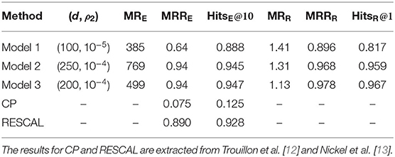
Table 1. Results for WordNet data analysis.

In addition to Models 1–3, we also display the performance of the Canonical Polyadic (CP) decomposition [22] and a tensor factorization approach, RESCAL [23]. Their MRR_E and Hits_E@10 results on the WordNet dataset are extracted from Trouillon et al. [12] and Nickel et al. [13], respectively. Both methods, especially CP, are outperformed by Model 3.

5. Concluding Remarks

In this article, we focused on the recovery of large-scale MRNs with a small portion of observations. We studied a generalized latent space model where entities and relations are associated with latent attribute vectors and conducted statistical analysis on the error of recovery. MLEs and pMLEs over a compact space are considered to estimate the latent attributes and the edge probabilities. We established non-asymptotic upper bounds for estimation error in terms of tail probability and risk, based on which we then studied the asymptotic properties when the size of MRN and latent dimension go to infinity simultaneously. A matching lower bound up to a log factor is also provided.

We kept ϕ generic for theoretical development. The choice of ϕ is usually problem-specific in practice. How to develop a data-driven method for selecting an appropriate ϕ is an interesting problem to investigate in future works.

Besides the latent space models, sparsity [24] or clustering assumptions [25] have been used to impose low-dimensional structures in single-relational networks. An MRN can be seen as a combination of several heterogeneous single-relational networks. The distribution of edges may vary dramatically across relations. Therefore, it is challenging to impose appropriate sparsity or cluster structures on MRNs. More empirical and theoretical studies are needed to quantify the impact of heterogeneous relations and to incorporate the information for recovering MRNs.

Data Availability Statement

The datasets generated for this study are available on request to the corresponding author.

Author Contributions

ZW provided the theoretical proofs. ZW and XT conducted the simulation and real data analysis. All authors contributed to manuscript writing and revision.

Funding

This work was supported by National Science Foundation grants SES-1826540 and IIS-1633360.

Conflict of Interest

The authors declare that the research was conducted in the absence of any commercial or financial relationships that could be construed as a potential conflict of interest.

Supplementary Material

The Supplementary Material for this article can be found online at: https://www.frontiersin.org/articles/10.3389/fams.2020.540225/full#supplementary-material

References

1. Miller GA. WordNet: a lexical database for English. Commun ACM. (1995) 38:39–41. doi: 10.1145/219717.219748

CrossRef Full Text | Google Scholar

2. McCray AT. An upper-level ontology for the biomedical domain. Compar Funct Genomics. (2003) 4:80–4. doi: 10.1002/cfg.255

PubMed Abstract | CrossRef Full Text | Google Scholar

3. Gabrilovich E, Markovitch S. Wikipedia-based semantic interpretation for natural language processing. J Artif Intell Res. (2009) 34:443–98. doi: 10.1613/jair.2669

CrossRef Full Text | Google Scholar

4. Scott S, Matwin S. Feature engineering for text classification. In: ICML Vol. 99 Bled (1999). p. 379–88.

5. Ferrucci D, Brown E, Chu-Carroll J, Fan J, Gondek D, Kalyanpur AA, et al. Building Watson: an overview of the DeepQA project. AI Mag. (2010) 31:59–79. doi: 10.1609/aimag.v31i3.2303

CrossRef Full Text | Google Scholar

6. Hoff PD, Raftery AE, Handcock MS. Latent space approaches to social network analysis. J Am Stat Assoc. (2002) 97:1090–8. doi: 10.1198/016214502388618906

CrossRef Full Text | Google Scholar

7. Bordes A, Usunier N, Garcia-Duran A, Weston J, Yakhnenko O. Translating embeddings for modeling multi-relational data. In: Burges CJC, Bottou L, Welling M, Ghahramani Z, Weinberger KQ, editors. Advances in Neural Information Processing Systems 26. Curran Associates, Inc. (2013). p. 2787–95. Available online at: http://papers.nips.cc/paper/5071-translating-embeddings-for-modeling-multi-relational-data.pdf

Google Scholar

8. Wang Z, Zhang J, Feng J, Chen Z. Knowledge graph embedding by translating on hyperplanes. In: AAAI. Québec City, QC (2014). p. 1112–9.

Google Scholar

9. Yang B, Yih SWt, He X, Gao J, Deng L. Embedding entities and relations for learning and inference in knowledge bases. In: Proceedings of the International Conference on Learning Representations. San Diego, CA (2015).

Google Scholar

10. Lin Y, Liu Z, Sun M, Liu Y, Zhu X. Learning entity and relation embeddings for knowledge graph completion. In: AAAI. Austin, TX (2015). p. 2181–7.

Google Scholar

11. Garcia-Duran A, Bordes A, Usunier N, Grandvalet Y. Combining two and three-way embedding models for link prediction in knowledge bases. J Artif Intell Res. (2016) 55:715–42. doi: 10.1613/jair.5013

CrossRef Full Text | Google Scholar

12. Trouillon T, Welbl J, Riedel S, Gaussier É, Bouchard G. Complex embeddings for simple link prediction. In: International Conference on Machine Learning. (2016). p. 2071–80.

Google Scholar

13. Nickel M, Rosasco L, Poggio TA. Holographic embeddings of knowledge graphs. In: AAAI. Phoenix, AZ (2016). p. 1955–61.

Google Scholar

14. Liu H, Wu Y, Yang Y. Analogical inference for multi-relational embeddings. In: Proceedings of the 34th International Conference on Machine Learning. Vol. 70. Sydney, NSW (2017). p. 2168–78.

Google Scholar

15. Socher R, Chen D, Manning CD, Ng A. Reasoning with neural tensor networks for knowledge base completion. In: Burges CJC, Bottou L, Welling M, Ghahramani Z, Weinberger KQ, editors. Advances in Neural Information Processing Systems. Lake Tahoe, NV: Curran Associates, Inc. (2013) p. 926–34.

Google Scholar

16. Kotnis B, Nastase V. Analysis of the impact of negative sampling on link prediction in knowledge graphs. arXiv. (2017) 170806816.

Google Scholar

17. Kanojia V, Maeda H, Togashi R, Fujita S. Enhancing knowledge graph embedding with probabilistic negative sampling. In: Proceedings of the 26th International Conference on World Wide Web Companion. Perth, WA (2017) p. 801–2. doi: 10.1145/3041021.3054238

CrossRef Full Text | Google Scholar

18. Min B, Grishman R, Wan L, Wang C, Gondek D. Distant supervision for relation extraction with an incomplete knowledge base. In: HLT-NAACL. Atlanta, GA (2013). p. 777–82.

Google Scholar

19. Zou H, Hastie T. Regularization and variable selection via the elastic net. J R Stat Soc B. (2005) 67:301–20. doi: 10.1111/j.1467-9868.2005.00503.x

CrossRef Full Text | Google Scholar

20. Duchi J, Hazan E, Singer Y. Adaptive subgradient methods for online learning and stochastic optimization. J Mach Learn Res. (2011) 12:2121–59. doi: 10.5555/1953048.2021068

CrossRef Full Text | Google Scholar

21. Robbins H, Monro S. A stochastic approximation method. Ann Math Stat. (1951) 22:400–7. doi: 10.1214/aoms/1177729586

CrossRef Full Text | Google Scholar

22. Hitchcock FL. The expression of a tensor or a polyadic as a sum of products. J Math Phys. (1927) 6:164–89. doi: 10.1002/sapm192761164

CrossRef Full Text | Google Scholar

23. Nickel M, Tresp V, Kriegel HP. A three-way model for collective learning on multi-relational data. In: Proceedings of the 28th International Conference on International Conference on Machine Learning. ICML'11. Madison, WI: Omnipress (2011). p. 809–16.

Google Scholar

24. Tran N, Abramenko O, Jung A. On the sample complexity of graphical model selection from non-stationary samples. IEEE Trans Signal Process. (2020) 68:17–32. doi: 10.1109/TSP.2019.2956687

CrossRef Full Text | Google Scholar

25. Jung A, Hero AO III, Mara AC, Jahromi S, Heimowitz A, Eldar YC, et al. Semi-supervised learning in network-structured data via total variation minimization. IEEE Trans Signal Process. (2019) 67:6256–69. doi: 10.1109/TSP.2019.2953593

CrossRef Full Text | Google Scholar