- 1Department of Mathematics, North Carolina State University, Raleigh, NC, United States
- 2Department of Physics, University of Oslo, Oslo, Norway
- 3Centre for Integrative Neuroplasticity, University of Oslo, Oslo, Norway
- 4Faculty of Science and Technology, Norwegian University of Life Sciences, Oslo, Norway
- 5Simula Metropolitan Center for Digital Engineering, Oslo, Norway
The local field potential (LFP) is the low frequency part of the extracellular electrical potential in the brain and reflects synaptic activity onto thousands of neurons around each recording contact. Nowadays, LFPs can be measured at several hundred locations simultaneously. The measured LFP is in general a superposition of contributions from many underlying neural populations which makes interpretation of LFP measurements in terms of the underlying neural activity challenging. Classical statistical analyses of LFPs rely on matrix decomposition-based methods, such as PCA (Principal Component Analysis) and ICA (Independent Component Analysis), which require additional constraints on spatial and/or temporal patterns of populations. In this work, we instead explore the multi-fold data structure of LFP recordings, e.g., multiple trials, multi-channel time series, arrange the signals as a higher-order tensor (i.e., multiway array), and study how a specific tensor decomposition approach, namely canonical polyadic (CP) decomposition, can be used to reveal the underlying neural populations. Essential for interpretation, the CP model provides uniqueness without imposing constraints on patterns of underlying populations. Here, we first define a neural network model and based on its dynamics, compute LFPs. We run multiple trials with this network, and LFPs are then analysed simultaneously using the CP model. More specifically, we design feed-forward population rate neuron models to match the structure of state-of-the-art, large-scale LFP simulations, but downscale them to allow easy inspection and interpretation. We demonstrate that our feed-forward model matches the mathematical structure assumed in the CP model, and CP successfully reveals temporal and spatial patterns as well as variations over trials of underlying populations when compared with the ground truth from the model. We also discuss the use of diagnostic approaches for CP to guide the analysis when there is no ground truth information. In comparison with classical methods, we discuss the advantages of using tensor decompositions for analyzing LFP recordings as well as their limitations.
1. Introduction
Most of what we know about the inner workings of the living brain has been learned from extracellular electrical recordings, that is, recordings of electrical potentials by sharp electrodes placed in the extracellular space between nerve cells. The high-frequency part of the signals, above a few hundred hertz, measures action potentials of neurons in the vicinity of the electrode contacts. The low-frequency part, the local field potential (LFP), is more difficult to interpret. While it is thought to mainly reflect processing of synaptic inputs by the neuronal dendrites by populations of pyramidal neurons, a simple rule-of-thumb interpretation in terms of the underlying neural activity like we have for spikes, is lacking [1, 2].
A traditional way to record LFPs in layered structures, such as hippocamapus or cortex is to record potentials with a linear multielectrode with many recording contacts crossing these laminarly organized brain structures. The resulting data typically have a two-way (matrix) structure (channels, time), and a standard analysis method has been to estimate the current-source density (CSD) [3]. The CSD measures the net volume density of electrical currents entering (sources) or leaving (sinks) the extracellular space. Several methods are available for CSD estimation, the standard CSD analysis assumes the neural activity to be constant in the horizontal directions in layered cortical or hippocampal structures [4], or other more recent methods like the iCSD [5] or the kCSD methods [6] which make different assumptions.
While the CSD is a more localized measure of neural activity than the LFP, it does not directly inform which neurons are active. An alternative is thus to try to decompose the measured LFPs into contributions from individual populations of neurons, for example, using matrix decomposition techniques like principal component analysis (PCA) [7] or independent component analysis (ICA) [8–10]. Here, data matrices are decomposed into outer products of pairs of vectors, and the vectors are interpreted as LFP contributions from individual neural populations. The decomposition of a matrix into outer products of vectors is not unique, and the methods involve additional assumptions like orthogonality (PCA) or statistical independence (ICA) of LFP contributions from the various populations. These mathematical assumptions cannot a priori be expected to be obeyed by neuronal populations in real brains. An alternative is to impose more physiological constraints in the decomposition [11]. An example is laminar population analysis (LPA) [12, 13] which, however, requires simultaneous recordings of action potentials and further physiological assumptions.
We here consider a new approach to LFP decomposition by considering three-way data (trial, channel, time) arranged as third-order tensors and performing a decomposition into outer products of triplets of vectors using an approach called CANDECOMP/PARAFAC (CP) [14, 15]. Unlike for the case with two-way data, this three-way decomposition is unique under mild conditions [16], and no strong assumptions, such as orthogonality or statistical independence on the components are needed. The underlying assumption in the CP model is that signals from each trial are a linear mixture of contributions from neural populations, and temporal and spatial signatures of neural populations stay the same across trials while each population's contribution to trials is scaled differently. Through the CP model, we assume that the LFP is multi-linear, thus linear in every argument (in our case tri-linear) since it assumes linearity in each mode. When matrix-based approaches, such as PCA and ICA are used on these signals from multiple trials by flattening the third-order LFP recording tensor, that structure cannot be maintained; therefore, additional assumptions, such as orthogonality are needed to ensure uniqueness.
Tensor decompositions are extensions of matrix decompositions, such as PCA to higher-order tensors (also referred to as multi-way arrays) and have proved useful in terms of finding underlying patterns in complex data sets in many domains including social network analysis, chemometrics, and signal processing [17–19]. As a result of its inherent uniqueness properties, among the tensor decomposition methods, the CP model has been quite popular since it can easily be interpreted. The CP model has also been successfully used in various neuroscience applications, e.g., the analysis of electroencephalography (EEG) signals [20], event related potential (ERP) estimation under the name topographic component analysis [21, 22], and more recently, capturing spatial, spectral, and temporal signatures of epileptic seizures [23, 24] and dynamics of learning [25].
In this study, we use the CP model to study LFP signals with the goal of disentangling individual neuronal populations. To the best of our knowledge, the CP model has not been used previously to analyze LFP recordings. In order to assess the performance of the CP model, we first create benchmarking data by simulating multi-channel LFP recordings across multiple trials based on a model of neuron populations. These simulated signals are arranged as a third-order tensor with modes: trials, channels, and time. Our numerical experiments demonstrate that the CP model can successfully reveal the underlying neuron populations by capturing their temporal and spatial signatures while more traditional ICA-based and PCA-based approaches fail to separate the populations. We also discuss advantages and limitations of the CP model in the presence of noise and different models of neuron populations.
2. Methods
In the methods section we first describe the forward model used to compute the model-based benchmarking data. This forward modeling consists of two parts: (i) a population firing-rate model simulating neural dynamics in a multi-population feed-forward network model, and (ii) the computation of the local field potential (LFP) stemming from these neural dynamics. Second, we describe the tensor decomposition approach used in the inverse modeling to reveal the individual neuronal populations.
2.1. Forward Modeling of Benchmarking Data
2.1.1. Rate Model for Neuron Populations
A neuron is a cell that processes and transmits information. It receives inputs called action potentials via synapses from pre-synaptic neurons. This input will change the internal state of the neuron (e.g., its membrane potential), and the neuron may itself generate action potentials that is forwarded to other post-synaptic neurons. One option for modeling dynamics of neural networks is to explicitly model the train of action potentials of all neurons in the network. For large neural networks this not only becomes numerically cumbersome, the results also become difficult to interpret.
Firing-rate models thus offer an attractive alternative: if the number of neurons grows, further simplifications can be used. Given a subset of all neurons which have similar properties, receive very similar input, and project to similar groups of neurons, we can call them a population. Instead of taking every action potential into account, the population activity can be described by their instantaneous firing rate, that is, the average number of action potentials fired in a time window across the population. This presents a huge simplification since the relative timing of all action potentials are neglected, but gives a description of larger population dynamics. In many cases the temporal evolution of the firing rate can be modeled by means of ordinary differential equations (ODE). For an extensive discussion of rate models, see, e.g., Ermentrout and Terman [26] and Gerstner et al. [27]. A population rate model for I neuron populations can be described by
where is the vector of instantaneous firing rates of I populations (thus restricted to non-negativity), the vector contains the time constants for each population, W ∈ ℝI × I is the coupling matrix describing the synaptic strength between populations, μ(t) is the instantaneous external stimulus received by each population and is the column-wise response function of each population to input (both from other neuron population as from external sources). The response function can in principle take any form and in general adds a non-linearity to the system. For simplicity we assume if not stated otherwise that is the identity function making the rate model fully linear.
The neural network is mainly characterized by the connection matrix W. If several populations affect each other only in a sequential way, we call these populations a feed-forward network. If several populations drive each other in a loop, we call those recurrent. If two neural populations are completely independent, meaning that they do not affect each other directly or indirectly via intermediate populations or do not share a common input, we can regard them as separate networks. One can further distinguish between excitatory and inhibitory neuron populations. Excitatory populations increase firing rate of post-synaptic populations, while inhibitory populations inhibit the firing of post-synaptic populations. Thus, Wi, j > 0 for all j if population i is excitatory and likewise Wi, j < 0 for i being an inhibitory population.
By assuming initial conditions r(0) and external stimuli μ(t), we fully define the ODE problem, which is solved using the ode45 package from MatLab [28]. We discretize dimensionless time between 0 and 1 in 1,000 steps and solve Equation (1) in this range. In this paper, we use a boxcar function
as stimulus with ci as the stimulus magnitude for each population i and and as the respective on and off-set for each population. Solving the rate model takes few seconds on a standard laptop and can thus be performed easily multiple times for different values of W and stimuli μ(t) to explore the model. Our choice of a linear model is a simplification which allows easier analysis, but has limitations, as, for example, it allows for (unphysical) negative firing rates.
2.1.2. Computation of LFP Signals
The local field potential (LFP) is the low-frequency part of extracellular potential, and in vivo it is generated from the superposition of the extracellular potential generated by many neurons [1]. The LFP Φ is a three-dimensional physical scalar field which can be continuously measured in time at any position, thus Φ(x, t). The LFP is measured by electrodes recording the signal at one or, more typically, many discrete locations, typically called channels. Thus, the recording becomes a vector of time series. In this discrete case, each LFP recording can thus be written as a matrix where the rows are the different channels and, the columns are the different discrete time points.
In this study, we mimic a situation where the LFP is recorded by a linear multielectrode at many positions through the depth of cortex. In this set-up, the recorded LFP will typically contain contributions from multiple populations of neurons with their somas (cell bodies) positioned at different depths (see, e.g., [12]). The multi-electrode probe records from multiple depth locations at the same time, and the spatial dependence x thus reduces to the scalar depth x, which simplifies further discussion. We do not aim to simulate any specific cortical system and instead keep things general. Therefore, we regard our model as a toy-model, which still incorporate key features of real LFPs. A method to efficiently compute LFPs is the so-called kernel method [29, 30].
The kernel method consists of several steps: (I) Biophysical, multi-compartment neuron models are used to generate a large number of neurons which then represent a set neuron populations. (II) All neurons in a single pre-synaptic population i are forced to emit an action potential at the same point in time. This mimics a δ-shaped firing rate. (III) The resulting LFP generated by each post-synaptic population j is stored separately for multiple locations, simulating a virtual probe with multiple channels. This provides a kernel Hij, the expected LFP if population i fires and projects to population j. (IV) Steps II and III are repeated for each pre-synaptic population i, providing a full set of kernels Hij. If W is constant, one can define the population kernel as the sum over all post-synaptic kernels . However, it is advantageous to maintain all Hi, j so that the contribution of individual populations to the total LFP can easily be computed.
The kernels Hi(x, t) thus depend on space x and time t, in the discrete case they can be represented as a matrix as well with dimensions channels and time. The LFP contribution of the ith population Φi(x, t) is computed by a temporal convolution of the corresponding kernel Hi(x, t) with the respective population firing rate ri(t):
Since the electrical potential is additive, the total LFP is given by summation over all populations
where * denotes the convolution operation in time and ri(t) is the firing rate of population i. In the discrete case, the result of the convolution is thus a matrix with the dimensions channel and time. This method has been developed as a part of the HybridLFPy software (see [29]). The kernels used in this work have been derived for a cat cortex model [31].
For each kernel Hi, there exists a rank-one approximation which allows to write the kernel as the outer product of a temporal ki and a spatial function ci:
where kT denotes the transposed vector. Since the projection of the neural population to the various channel locations is determined by their static morphology and the propagation of the electrical signal through neurons is fast, there is little delay at different locations. Therefore, the rank-one approximation is very accurate (variance explained above 95% for all studied cortical kernels, see Appendix). Due to this factorization of the kernel into spatial and temporal parts, the resulting LFP can also be factorized in a spatial and temporal part since the firing rate is only convolved with the kernel in the temporal dimension:
where * denotes the convolution operator. If we discretize, spatial and temporal factors of the kernel become vectors: ci(x) → ci, ki(t) → ki, and the kernel itself turns into a matrix Hi(x, t) → Hi. Since the population firing rate r(t) is also solved numerically, the continuous solution turns into a vector ri(t) → ri. Thus, the LFP (Equation 6) can be written as a matrix Φ ∈ ℝM × N:
with M as the number of channels and N as the number of time points. By repeating the simulation of Φ multiple (L) times, e.g., for different connection matrices W mimicking changes of the network over time, and stack the resulting LFPs, we get a three-way tensor with modes: trials, channels, and time.
2.2. CANDECOMP/PARAFAC (CP) Tensor Model Used in Inverse Modeling
The CP model, also known as the canonical polyadic decomposition [32], is one of the most popular tensor decomposition approaches. Here, we use the CP model to analyze the three-way LFP tensor with modes: trials, channels, and time, and reveal temporal and spatial signatures of underlying neuron populations. For a third-order tensor (three-way array) , an R-component CP model approximates the tensor as the sum of R rank-one third-order tensors, as follows:
where ∘ denotes the vector outer product following the notation in Kolda and Bader [17], correspond to factor matrices in trials, channels, and time mode, respectively. Note that the outer product of three vectors is a third-order rank-one tensor, i.e., . The CP model is unique under mild conditions up to permutation and scaling [16, 17]; in other words, the same rank-one components, i.e., sr∘cr∘tr, for r = 1, …, R, are revealed by the model at the solution but the order of rank-one components is arbitrary and within each rank-one component, factor vectors have a scaling ambiguity, e.g., 2sr ∘ 1/2cr ∘ tr. By normalizing columns of the factor matrices and introducing an additional scalar, λr, for each rank-one component, we can rewrite Equation (8) as follows:
with , , and as unit-norm factor vectors.
The CP model is considered to be one way of extending Singular Value Decomposition (SVD) to higher-order data sets. As a result of its uniqueness properties, the CP model has the benefit of revealing underlying patterns without imposing strict and potentially unrealistic constraints, such as orthogonality or statistical independence as in the case of matrix decomposition-based approaches, such as PCA and ICA. When an R-component CP model is used to analyze an LFP tensor, it extracts R rank-one components.
Our motivation for using the CP model to analyze LFP tensors is as follows: If the population rate model is fully linear ( in Equation 1 is a linear function), then the solutions of equation (Equation 1) are only linearly dependent of the connection matrix W and/or the external stimulus μ(t). If trials with variations of W and/or μ(t) are performed, the resulting firing rates will thus only depend linearly on W and μ(t). Furthermore, if we also assume that kernels are rank-one matrices, fulfilling Equation (5), a tensor consisting of multiple trials of multi-electrode LFP recordings will have an underlying CP structure (see Equations 7 and 8).
We claim that these extracted tensor components correspond to spatial and temporal signatures of neuron populations, i.e., cr and tr correspond to spatial and temporal signatures of the rth population (see Equation 7), due to the fact that the LFP of each population can be written as a bi-linear form and given the uniqueness of CP. Each component in the CP thus corresponds to a neural population.
Given the number of components R, in order to fit a CP model to a third-order tensor , we solve the following optimization problem:
where ‖·‖F denotes the Frobenius norm for tensors, i.e., . There are various algorithmic approaches for solving this problem, such as alternating least squares (ALS) and all-at-once optimization methods. In this paper, we use a gradient-based all-at-once approach based on CP-OPT [33], that solves the problem for all factor matrices, S, C, T, simultaneously.
2.2.1. Diagnostics Tools
Determining the number of CP components (R) is a difficult problem. For the exact case, where there is an equality in Equation (8), R corresponds to the tensor rank and determining the rank of a tensor is NP-hard [17, 34]. In practice, this challenging problem has been mitigated using various diagnostic tools, such as core consistency diagnostic [35], split-half and residual analysis [36]. In this paper, we use the core consistency values and model fit to determine the number of components while modeling an LFP tensor using a CP model.
Core Consistency indicates whether an R-component CP model is an appropriate model for the data, and is defined as follows [35]:
where (of size R × R × R) is the estimated core array for a Tucker model [37] given the factor matrices of the R-component CP model, and (of size R × R × R) is a super-diagonal core array for the CP model with non-zero entries only on the super-diagonal. Tucker is a more flexible tensor model; therefore, its core can be a full core array. If the R-component CP model is a valid model, then off super-diagonal elements of will be close to zero giving high core consistency values close to 100%. Low core consistency values indicate potentially an invalid CP model.
Model Fit is used to understand how much of the data is explained by the model. Given a tensor and its CP approximation , the fit can be defined as follows:
When the number of components extracted from the data increases, the fit also increases. However, the increase in additional complexity due to additional components should often be justified by an increase in model fit. In other words, we need to assess if we gain a significant increase in fit by extracting more components from the data.
To find the optimal number of components R, we examine model fit and core consistency values across different number of components. While heuristic in nature, these diagnostics are able to be employed effectively in this study.
3. Numerical Experiments
As an example, we assume the simple model of four neuron populations which are sequentially connected (see Figure 1). Population 1 receives the same stimulus in every trial l while the other populations only receive indirect input via projections from other populations (). We further assume that the network is purely excitatory (0 ≤ Wij). We model multiple trials by assuming that due to plasticity, W21, W32, and W43 will change between trials. This mimics the situation where a subject is exposed to the same stimulus at different times and the neural network adapts and changes its connectivity due to learning. This plasticity is not part of our model, but externally enforced. We will show that the changes in weights across trials can be recovered using the CP model and thus will allow to study the learning process.

Figure 1. Sketch of a four-population feed-forward neural model defined via connection matrix in Equation (11) .
This network has the following sparse connectivity matrix:
To indicate different trials, we use superscripts, e.g., Wl is the connection matrix for the lth trial. We define the experimental population strength as the strength of the rth population in the lth trial. For the four population feed-forward model, we thus have the relation
Since the convolution with the temporal factor of the kernel kr (see Equation 7) is also a linear operation and the channel factor cr does not change between trials, we expect that when multi-trial multi-electrode LFP signals from this model are analyzed using an R-component CP model, the analysis will reveal the following:
• The trial population strength matrix (s1, s2, …, sR)
• The channel factor matrix (c1, c2, …, cR)
• The temporal factor matrix (r1*k1, r2*k2, …, rR*kR)
Note that it is only possible to recover (1) the experimental population strength (see Equation 12), not the connection matrix entries W, and (2) the time-convolved temporal components (rr*kr = tr) instead of the raw time traces rr. In the following, we will refer to the time-convolved components simply as the time components. To perform numerical simulations, we impose learning by a controlled change of W. Over a set of L = 30 trials, we modulate W21 with a sinusoidal and an offset, such that over the trials, it performs a quarter period (. W32 increases linearly () and W43 decreases linearly (. We arbitrary set τ = (0.1, 0.3, 0.3, 0.2))T and stimulate with a boxcar (Equation 2) between 0 and 0.2 (tstart = 0, tend = 0.2). Here, we simulate multi-electrode LFP recordins across multiple trials based on a simple population rate model, and arrange the data as an LFP tensor with modes: trials, channels, and time. We then analyze the LFP tensor using an R-component CP model to disentangle R populations by estimating their spatial signatures (cr), temporal signatures (tr) and relative contributions to trials (sr), for r = 1, ..., R.
In order to demonstrate the performance of the CP model in terms of analyzing LFP tensors, we have constructed the following tensors (all in the form of 30 trials × 16 channels × 1,000 time points):
(i) A noise-free data set using full kernels: An LFP data set simulated by using the full kernels (Equation 4). No noise was added to the simulation.
(ii) A noise-free simulation using rank-one approximation of kernels: An LFP data set was simulated using the rank-one approximation of the kernels for each population (Equation 5). Let be the SVD of kernel of rank R for population i. Its rank-one approximation is . The rank-one approximation of each selected kernel explains over 95% of the kernel matrix. No noise was added to the simulation.
(iii) Noisy LFP with rank-one approximation of kernels: LFP data set was simulated using the rank-one approximation of kernels and then added noise as follows: Let denote the LFP tensor that is constructed using the rank-one kernel approximations. The noisy LFP tensor with noise level α is given by where is a tensor with entries randomly drawn from the standard normal distribution.
Constructed LFP tensors are then analyzed using CP with different number of components. We have also compared the performance of the CP model with ICA and PCA.
3.1. Implementation Details
For fitting the CP model, cp_opt from the Tensor Toolbox [38] using the non-linear conjugate gradient (NCG) algorithm, as implemented in the Poblano Toolbox [39] is used. Multiple initializations are used to fit each R-component CP model, and the solution with the best function value is reported. For computing core consistency values, we use the corcond function from the Nway Toolbox [40].
For ICA, we use two different algorithms: (i) FastICA [41] exploiting non-Gaussianity of the underlying sources, and (ii) the ERBM (entropy-rate bound minimization) [42] algorithm that takes into account both higher-order statistics and sample dependence to find the underlying sources. For ICA algorithms, again multiple initializations are used with R components and among all the runs, we report the one that matches the true factors best.
3.2. Performance Evaluation
In order to assess the performance of the CP model, we quantify the similarity between CP factors and true signatures of neuron populations in trials, channels, and time modes. We use the Factor Match Score (FMS) as the similarity measure defined as follows [33, 43]:
where for r = 1, ..., R denote the estimated components by the CP model while sr, cr, tr for r = 1, ..., R denote the true components, i.e., simulated trials, channels, and time mode factors.
3.3. Results
Using numerical experiments, we demonstrate that the CP model can successfully extract components revealing each population. The model succeeds in revealing the populations from the noise-free tensor constructed using full kernels and also from the noise-free tensor constructed using rank-one approximation of kernels. In the presence of noise, each population can still be unraveled while their signatures are distorted by the noise. For the first type of tensor constructed using full kernels, the 4-component CP model can successfully capture the true factors as shown in Figure 2. Note that even though the tensor is constructed with full kernels, the true components in channels and time modes are assumed to be the leading singular vectors of each kernel matrix under the assumption that kernels have a rank-one structure with noise. Under this assumption, when true components and CP components are compared quantitatively, the FMS is 0.9965 indicating the accurate recovery of true patterns using the CP model. Here, the optimal number of components is equivalent to the number of populations that contribute to the data; therefore R = 4. We have also analyzed the data using CP with different number of components. Figure 3 shows how core consistency and model fit change with R. Since we expect high core consistency values for valid CP models, we increase the number of components until we see a drop in core consistency. Both R = 4 and R = 5 potentially look valid models; however, the model fit is already 100% for R = 4 and becomes flat after R = 4 indicating that the 4-component CP model is the right choice. Thus, we are able to identify the correct number of neural populations based on the diagnostic tools used for determining the number of CP components.
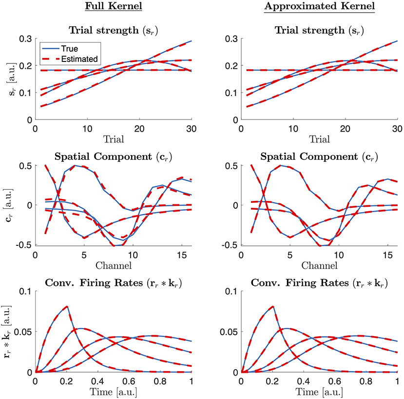
Figure 2. True (simulated) components (blue solid line) vs. the factor vectors extracted by a 4-component CP model (red dashed) in trials, channels, and time modes from a tensor constructed via full kernels (left column) and rank one approximated kernels (right column). Note also that what is extracted by the CP model is which is then compared with rr*kr from the benchmarking data.
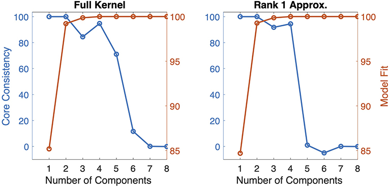
Figure 3. Core consistency and model fit for CP models with R = 1, 2, …, 8 components for tensors constructed with full kernels and the rank-one approximations of kernels.
In the second case, where a tensor is constructed via the best rank-one approximation of each kernel, the 4-component CP model can again unravel the four populations and their corresponding signatures in trials, channels, and time modes as shown in Figure 2. Core consistency and model fit values shown in Figure 3 for different number of components and, in this case, indicate that R = 4 is the true number of components since the core consistency significantly drops after R = 4. Again, the true number of components could be identified using diagnostic tools.
When noise is added to the tensor constructed using rank-one approximated kernels, the CP model (with R = 4 components) can still reveal the true signatures of the populations; however, as we increase the noise level, we observe that factors become distorted as shown in Figure 4. Table 1 shows that FMS values are still high for different levels of noise, and the model fit decreases as a result of the noise, as expected. Core consistency values, however, are much lower and therefore indicate noisy components.
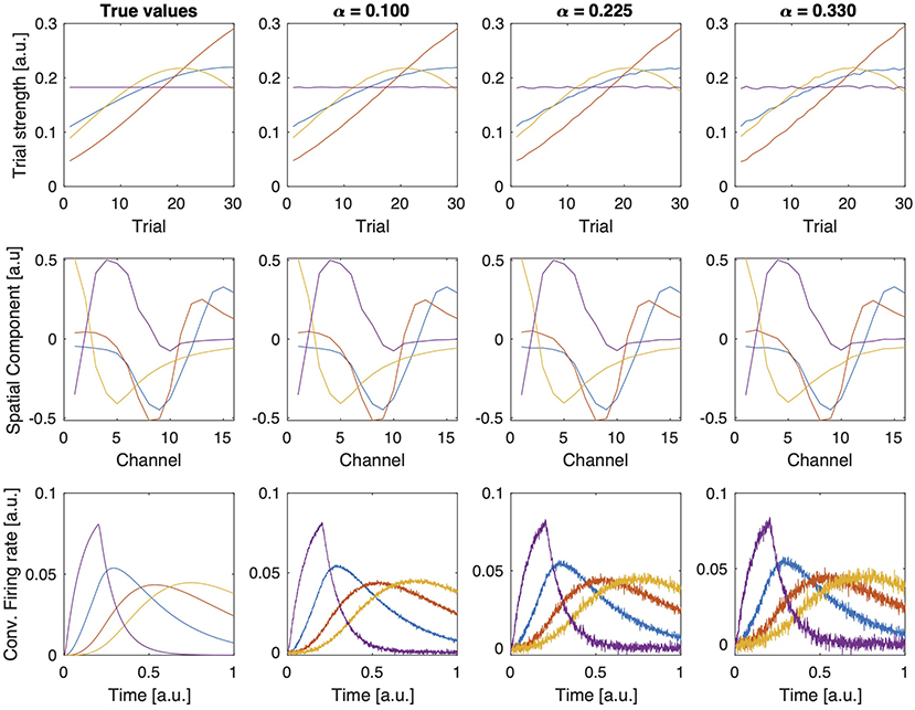
Figure 4. Factor vectors in each mode of a 4-component CP model of tensors with different noise levels (α).
3.4. Comparisons With ICA and PCA
Since ICA and PCA are more traditional approaches to analyze multi-channel electro-physiology data, we compare the performance of CP with both in terms of how well they recover the true temporal components. For ICA and PCA, we unfold the third-order LFP tensor in the time mode and arrange the data as a trials-channels by time matrix. In our comparisons, we use two different ICA algorithms: The FastICA algorithm [44] and the ERBM algorithm [42]. We study the noise-free case, analyze the LFP tensor using the correct number of underlying populations with CP, ICA (R = 4), and PCA, and compare the estimated sources in the time dimension in Figure 5. FastICA only finds two independent components, even if the correct larger number is given. The two reconstructed components do not mimic the actual firing rate components. The ERBM algorithm was able to reconstruct two components which are similar to the ground truth, but the other two components do not match the ground truth. The unfolded noise-free tensor is of rank four, and when all four components were taken into account, PCA was able to recover the first component to some extent, but failed in the other components. The CP model, on the other hand, was able to recover all four components with high accuracy. This is a clear example that illustrates the advantage of using CP over classical matrix methods. Furthermore, the CP model also allows to estimate the components in trials and channels modes, whereas matrix-based methods like ICA or PCA require an unfolding of the tensor, therefore, failing to estimate components in all modes simultaneously.
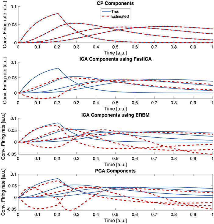
Figure 5. Comparing CP, FastICA, ERBM, and PCA estimates of temporal components. Data was generated without additional noise and the correct number of components was provided to the algorithms.
3.4.1. Further Interpretation
We have shown that CP is able to blindly recover the location of each population (cr), but can only recover the population firing rate convolved with the temporal part of the corresponding kernel (rr*kr). There is no method available which blindly can deconvolve the kernel and firing rate. The potential kernel kr can be constrained by values found in experimental studies. Performing standard deconvolution algorithms [45] can then be used to further estimate the actual population firing rate. Another limitation of the blind CP approach is that it can only recover the trial population strength sr, but not the underlying connectivity matrix W due to the relation in Equation (12). If one assumes a feed-forward network, a relation as described in Equation (12) can be assumed, but the order of components is arbitrary by CP. Inspection of the firing rate components (see for example Figure 4) can reveal a causal connection (purple → blue → red → yellow) and identify the order of components. Then, the elements of W can be recovered by the simple iteration . Also, if two neuron populations have identical synaptic projection patterns, their LFP kernels will be also identical, making it impossible to distinguish them. Therefore, clearly identifying the spatial location of population LFPs relies on the assumption that their projection patterns are different.
3.5. Application to a Non-linear Model
As stated in section 2.2, the assumption that a tensor consisting of multiple trials of multi-electrode LFP recordings will have an underlying CP structure relies on the assumption that (Equation 1) is linear. However, in general will be non-linear. To study the effects of introducing non-linearity, we use a hyperbolic tangent function as suggested by beim Graben and Kurths [46] instead of the identity function. To study the gradual increase of non-linearity, our function is set to be in the form of
with a = 0.5 so that the inflection is within the range of inputs, and to ensure that . In this form, the parameter β can be thought to represent the strength of the non-linearity of the system. For small values of β, is approximately the identity function. As the value of β increases becomes more non-linear. Effects of the parameter β on the convolved firing rates can be seen in Figure 6. Results of CP decomposition of the LFP tensor generated with increasing non-linearity (β) can be seen in Figure 7 with associated factor match scores. Factor match scores are computed assuming that the mean of the firing rates of each population across trials is the ground truth. We observe FMS of 0.9995, 0.9964, and 0.7497 for β = 0.001, 1, and 5, respectively. Note that with a weak non-linearity, CP is able to recover components that are close to the mean of the trials, thus the non-linearity can be regarded as a small perturbation. In this case CP is stable and can produce reasonable results. If the non-linearity becomes too strong, CP will, as expected, eventually fail, as shown in Figure 7. Thus, CP will provide a linear approximation of the data.
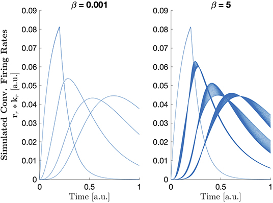
Figure 6. Normalized convolved firing rates from all trials with and β = 0.001 (left) and β = 5 (right).
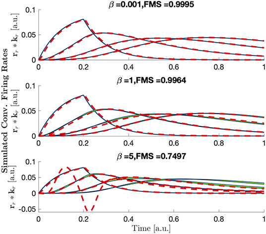
Figure 7. The mean ± 3 standard deviations of each population's convolved firing rate across trials (blue) with area between the two curves shaded in green and CP reconstruction plotted as dashed red lines for increasing amounts of non-linearity. Larger green regions represent larger shape changes in the normalized firing rates.
Also note that CP without non-negativity constraints reveal temporal components with negative values. In the Appendix (Figure A3), we also show the temporal factors obtained using a CP model with non-negativity constraints in the time and trial mode, for the different strength of non-linearity. We observe that for small non-linearities, where CP gives reasonable (and already non-negative) components, non-negativity constraint has almost no effect. In cases of strong non-linearity where CP fails, the constraint results in very different results.
4. Discussion
4.1. Summary of Findings
In this paper we have applied the CP tensor decomposition approach to disentangle different neural populations in LFP recordings from multiple trials. The idea behind the CP model is that signals from each trial are a mixture of signals from several neural populations with specific temporal and spatial patterns. While these population-specific patterns stay the same across trials, contributions of the populations are scaled differently from one trial to another. By jointly analyzing signals from multiple trials, the CP model can uniquely reveal the underlying neural populations and capture population-specific temporal and spatial signatures without imposing ad hoc constraints on those patterns like what is required for using PCA and ICA. Physiologically, we have made several assumptions. We first assume that if a neural population receives the same input but with different magnitude in multiple trials, than its firing will also be the same, but with a different magnitude proportional to the input magnitude, thus we assume linear response of the population. Second, we assume that the location, and thus the recording channels a certain population projects to, is constant over time and also does not change between trials. Last, we assume that our input dominates the network activity and background processes ongoing in the network can be regarded as noise.
We used a linear feed-forward firing-rate toy model with four populations in this study. The LFP was computed by means of a kernel method, which allowed simple and fast generation of LFP given the population activity of neurons in the model. By repeating the model with different synaptic weights and the same stimulus, we generated a multi-trial, multi-channel time series tensor of LFP recordings. For this toy-model, we found that CP works very well and is able to recover the temporal, spatial and trials modes of the model as shown in Figure 2. This decomposition is unique, which allows interpretation of those components as the neural populations. We also found that the method is robust against noise. Even if the noise is reflected in the components, the components still cover the main feature of the model as shown in Figure 4. We were able to uncover the true number of components using the core consistency diagnostic (see Figure 3). For applications with experimental recordings where the number of components is not known, the core consistency diagnostic is often an effective way to estimate the correct number of components.
4.2. Comparison With Classical Matrix Factorization Methods
Different ICA methods and PCA were not able to fully recover the true components corresponding to individual populations. ICA relies on the strong assumption of statistical independence of components, even if that is relaxed in the ERBM approach. In a biological network, this assumption is unlikely to be met since it is expected to process and integrate information, thus correlated patterns are expected. We suspect that ICA methods failed because of highly correlated component vectors in the time mode. PCA tried to minimize the correlation between components, which is unlikely to be met in a neural network. On the other hand, CP does not rely on the assumption of independence and is, therefore, able to recover the components successfully. Also, ICA and PCA methods work on signals arranged as matrices, which requires unfolding the tensor. Unfolding destroys the multi-linear structure the CP model benefits from, and ICA/PCA cannot make use of that structure.
4.3. Extensions of CP Model for Different Models of Neuronal Populations Activity
In our toy feed-forward model, the data had a low-rank CP structure and a CP decomposition was able to fully recover it. We also studied the result of introducing non-linear neural response and showed that, for a small amount of non-linearity, CP is able to identify populations. However, for larger non-linearities we see the failure of the CP method as the data violates the CP assumptions to a larger extent. In a more realistic model, we can introduce recurrent connections, multiple simultaneous inputs and non-linear response of neural populations. In such cases, in particular for the second case, using a CP model would lead to uniqueness issues due to linearly dependent components. For instance, this can occur when two different stimuli are injected in the network, thus each stimulus in each neural population would correspond to a single component, but all components related to the same neural population would have the same channel factor. Generalizations of the CP model, e.g., the Tucker model [17], are flexible enough to cover this. While not unique by construction, additional constraints, such as non-negativity, sparsity or the structure of the Tucker core can allow for uniqueness.
When CP is applied to experimental LFP recordings like in Verleger et al. [22], it is unlikely that a low-rank approximation will fully explain the recording due to multiple external sources, contributions from other brain regions, noise effects and non-linearity of the system. However, even if CP is not capable to model the entire data using a low-rank approximation, CP will still pick up low-rank parts, such as a feed-forward structure and thus make it possible to understand sub-structures of the network.
4.4. Measurements Other Than LFP Signal
Other multi-electrode recordings like EEG, electrocorticography (ECoG) or magnetoencephalography (MEG) are very similar to LFP in the sense that they also consist of contributions of multiple sources. Due to the linearity of electromagnetism, these contributions are also additive. Recent work [47] allows to simulate not only LFP but also other electrophysiological signals in the same framework. Thus, the kernel method can also be applied to these other observables. If the kernels have a good rank-one approximation, this work would also apply to EEG, ECoG, or MEG. Since all those observables are linked by the same underlying population activity, it is also possible to combine several observables in a fusion framework jointly analyzing multiple tensors [48].
Data Availability Statement
The simulation and analysis scripts for this study can be found here https://github.com/CINPLA/MultiLinearPopulationAnalysis-MLPA. We put the final code here.
Author Contributions
EA and AS conceived and conceptualized the project. JG, EA, and AS wrote and executed all the codes for simulating and analysing the data. JG, EA, GE, and AS wrote the paper. All authors contributed to the article and approved the submitted version.
Funding
JG has been funded by the National Science Foundation under the award NSF/DMS(RTG) #1246991. GE, EA, and AS have been funded by the Research Council of Norway (NFR) through the following projects: GE [project# 250128 (COBRA)], EA [project# 300489 (IKTPLUSS)], and AS [project# 250128 (COBRA) and 300504 (IKTPLUSS)].
Conflict of Interest
The authors declare that the research was conducted in the absence of any commercial or financial relationships that could be construed as a potential conflict of interest.
Acknowledgments
We would like to thank Espen Hagen for providing the kernels for this study.
References
1. Einevoll GT, Kayser C, Logothetis NK, Panzeri S. Modelling and analysis of local field potentials for studying the function of cortical circuits. Nat Rev Neurosci. (2013) 14:770–85. doi: 10.1038/nrn3599
2. Pesaran B, Vinck M, Einevoll GT, Sirota A, Fries P, Siegel M, et al. Investigating large-scale brain dynamics using field potential recordings: analysis and interpretation. Nat Neurosci. (2018) 21:903–19. doi: 10.1038/s41593-018-0171-8
3. Pettersen KH, Lindén H, Dale AM, Einevoll GT. Extracellular spikes and CSD. In: Brette R, Destexhe A, editors. Handbook of Neural Activity Measurement. Cambridge: Cambridge University Press (2012). p. 92–135. doi: 10.1017/CBO9780511979958.004
4. Nicholson C, Freeman JA. Theory of current source-density analysis and determination of conductivity tensor for anuran cerebellum. J Neurophysiol. (1975) 38:356–68. doi: 10.1152/jn.1975.38.2.356
5. Pettersen KH, Devor A, Ulbert I, Dale AM, Einevoll GT. Current-source density estimation based on inversion of electrostatic forward solution: effects of finite extent of neuronal activity and conductivity discontinuities. J Neurosci Methods. (2006) 154:116–33. doi: 10.1016/j.jneumeth.2005.12.005
6. Helena. Kernel current source density method. Neural Comput. (2012) 24:541–75. doi: 10.1162/NECO_a_00236
7. Barth DS, Di S. Laminary excitability cycles in neocortex. J Neurophysiol. (1991) 65:891–8. doi: 10.1152/jn.1991.65.4.891
8. Leski S, Kublik E, Swiejkowski Da, Wróbel A, Wójcik DK. Extracting functional components of neural dynamics with independent component analysis and inverse current source density. J Comput Neurosci. (2010) 29:459–73. doi: 10.1007/s10827-009-0203-1
9. Makarov VA, Makarova J, Herreras O. Disentanglement of local field potential sources by independent component analysis. J Comput Neurosci. (2010) 29:445–57. doi: 10.1007/s10827-009-0206-y
10. Głçbska H, Potworowski J, Łçski S, Wójcik DK. Independent components of neural activity carry information on individual populations. PLoS ONE. (2014) 9:e105071. doi: 10.1371/journal.pone.0105071
11. Gratiy SL, Devor A, Einevoll GT, Dale AM. On the estimation of population-specific synaptic currents from laminar multielectrode recordings. Front Neuroinform. (2011) 5:32. doi: 10.3389/fninf.2011.00032
12. Einevoll GT, Pettersen KH, Devor A, Ulbert I, Halgren E, Dale AM. Laminar population analysis: estimating firing rates and evoked synaptic activity from multielectrode recordings in rat barrel cortex. J Neurophysiol. (2007) 97:2174–90. doi: 10.1152/jn.00845.2006
13. Glabska HT, Norheim E, Devor A, Dale AM, Einevoll GT, Wojcik DK. Generalized laminar population analysis (gLPA) for interpretation of multielectrode data from cortex. Front Neuroinform. (2016) 10:1. doi: 10.3389/fninf.2016.00001
14. Harshman RA. Foundations of the PARAFAC procedure: models and conditions for an explanatory multi-modal factor analysis. UCLA Work Pap Phonet. (1970) 16:1–84.
15. Carroll JD, Chang JJ. Analysis of individual differences in multidimensional scaling via an N-way generalization of “Eckart-Young” decomposition. Psychometrika. (1970) 35:283–319. doi: 10.1007/BF02310791
16. Kruskal JB. Three-way arrays: rank and uniqueness of trilinear decompositions, with application to arithmetic complexity and statistics. Linear Algebra Appl. (1977) 18:95–138. doi: 10.1016/0024-3795(77)90069-6
17. Kolda TG, Bader BW. Tensor decompositions and applications. SIAM Rev. (2009) 51:455–500. doi: 10.1137/07070111X
18. Acar E, Yener B. Unsupervised multiway data analysis: a literature survey. IEEE Trans Knowl Data Eng. (2009) 21:6–20. doi: 10.1109/TKDE.2008.112
19. Papalexakis EE, Faloutsos C, Sidiropoulos ND. Tensors for data mining and data fusion: models, applications, and scalable algorithms. ACM Trans Intell Syst Technol. (2016) 8:Article 16. doi: 10.1145/2915921
20. Cole HW, Ray JW. EEG correlates of emotional tasks related to attentional demands. Int J Psychophysiol. (1985) 3:33–41. doi: 10.1016/0167-8760(85)90017-0
21. Möcks J. Topographic components model for event-related potentials and some biophysical considerations. IEEE Trans Biomed Eng. (1988) 35:482–4. doi: 10.1109/10.2119
22. Verleger R, Paulick C, Möcks J, Smith JL, Keller K. Parafac and go/no-go: disentangling CNV return from the P3 complex by trilinear component analysis. Int J Psychophysiol. (2013) 87:289–300. doi: 10.1016/j.ijpsycho.2012.08.003
23. Acar E, Bingol CA, Bingol H, Bro R, Yener B. Multiway analysis of epilepsy tensors. Bioinformatics. (2007) 23:i10–8. doi: 10.1093/bioinformatics/btm210
24. De Vos M, Vergult A, De Lathauwer L, De Clercq W, Van Huffel S, Dupont P, et al. Canonical decomposition of ictal scalp EEG reliably detects the seizure onset zone. Neuroimage. (2007) 37:844–54. doi: 10.1016/j.neuroimage.2007.04.041
25. Williams AH, Kim TH, Wang F, Vyas S, Ryu SI, Shenoy KV, et al. Unsupervised discovery of demixed, low-dimensional neural dynamics across multiple timescales through tensor component analysis. Neuron. (2018) 98:1099–115. doi: 10.1016/j.neuron.2018.05.015
26. Ermentrout GB, Terman DH. Mathematical Foundations of Neuroscience. Vol. 35.Springer Science & Business Media (2010).
27. Gerstner W, Kistler WM, Naud R, Paninski L. Neuronal Dynamics: From Single Neurons to Networks and Models of Cognition. Cambridge: Cambridge University Press (2014). doi: 10.1017/CBO9781107447615
29. Hagen E, Dahmen D, Stavrinou ML, Lindén H, Tetzlaff T, van Albada SJ, et al. Hybrid scheme for modeling local field potentials from point-neuron networks. Cereb Cortex. (2016) 16:P67. doi: 10.1186/1471-2202-16-S1-P67
30. Skaar JEW, Stasik AJ, Hagen E, Ness TV, Einevoll GT. Estimation of neural network model parameters from local field potentials (LFPs). PLoS Comput Biol. (2020) 16:e1007725. doi: 10.1371/journal.pcbi.1007725
31. Potjans T, Diesmann M. The cell-type specific cortical microcircuit: relating structure and activity in a full-scale spiking network model. Cereb Cortex. (2012) 24:785–806. doi: 10.1093/cercor/bhs358
32. Hitchcock FL. The expression of a tensor or a polyadic as a sum of products. J Math Phys. (1927) 6:164–89. doi: 10.1002/sapm192761164
33. Acar E, Dunlavy DM, Kolda TG. A scalable optimization approach for fitting canonical tensor decompositions. J Chemometr. (2011) 25:67–86. doi: 10.1002/cem.1335
34. Håstad J. Tensor rank is NP-complete. J Algorithms. (1990) 11:644–54. doi: 10.1016/0196-6774(90)90014-6
35. Bro R, Kiers HAL. A new efficient method for determining the number of components in PARAFAC models. J Chemometr. (2003) 17:274–86. doi: 10.1002/cem.801
36. Bro R. PARAFAC. Tutorial and applications. Chemometr Intell Lab Syst. (1997) 38:149–71. doi: 10.1016/S0169-7439(97)00032-4
37. Tucker LR. Some mathematical notes on three-mode factor analysis. Psychometrika. (1966) 31:279–311. doi: 10.1007/BF02289464
38. Bader BW, Kolda TG. MATLAB Tensor Toolbox Version 3.1. (2019). Available online at: https://www.tensortoolbox.org
39. Dunlavy DM, Kolda TG, Acar E. Poblano v1.0: A Matlab Toolbox for Gradient-Based Optimization. Albuquerque, NM; Livermore, CA: Sandia National Laboratories (2010).
40. Andersson CA, Bro R. The N-way toolbox for MATLAB. Chemometr Intell Lab Syst. (2000) 52:1–4. doi: 10.1016/S0169-7439(00)00071-X
41. Hyvärinen A. Fast and robust fixed-point algorithms for independent component analysis. IEEE Trans Neural Netw. (1999) 10:626–34. doi: 10.1109/72.761722
42. Li XL, Adali T. Blind spatiotemporal separation of second and/or higher-order correlated sources by entropy rate minimization. In: ICASSP'2010: Proceedings of IEEE International Conference on Acoustics, Speech, Signal Processing. Dallas, TX (2010). p. 1934–7. doi: 10.1109/ICASSP.2010.5495311
43. Tomasi G, Bro R. A comparison of algorithms for fitting the PARAFAC model. Comput Stat Data Anal. (2006) 50:1700–34. doi: 10.1016/j.csda.2004.11.013
44. Hyvärinen A, Oja E. Independent component analysis: algorithms and applications. Neural Netw. (2000) 13:411–30. doi: 10.1016/S0893-6080(00)00026-5
45. Virtanen P, Gommers R, Oliphant TE, Haberland M, Reddy T, Cournapeau D, et al. SciPy 1.0: fundamental algorithms for scientific computing in Python. Nat Methods. (2020) 17:261–72. doi: 10.1038/s41592-019-0686-2
46. beim Graben P, Kurths J. Simulating global properties of electroencephalograms with minimal random neural networks. Neurocomputing. (2008) 71:999–1007. doi: 10.1016/j.neucom.2007.02.007
47. Hagen E, Næss S, Ness TV, Einevoll GT. Multimodal modeling of neural network activity: computing LFP, ECoG, EEG, and MEG signals with LFPy 2.0. Front Neuroinform. (2018) 12:92. doi: 10.3389/fninf.2018.00092
48. Acar E, Schenker C, Levin-Schwartz Y, Calhoun VD, Adali T. Unraveling diagnostic biomarkers of schizophrenia through structure-revealing fusion of multi-modal neuroimaging data. Front Neurosci. (2019) 13:416. doi: 10.3389/fnins.2019.00416
Appendix
Kernels for LFP Approximation
The kernels used in this work were computed as described in Hagen et al. [29] for a cat cortex model [31]. We selected a random sequence of only excititory kernels where we made sure that the first kernel projects from talamic input. We used the following kernels: thalamus → layer 4, layer 4 → layer 6, layer 6 → layer 5, and layer 5 → layer 2/3. Kernels were computed with ±20ms around the δ input. Due to causality, no response is expected before the pulse. Figure A1 shows the selected kernels as well as their rank one approximation. As it can be seen, a rank one approximation approximates the original kernel well.
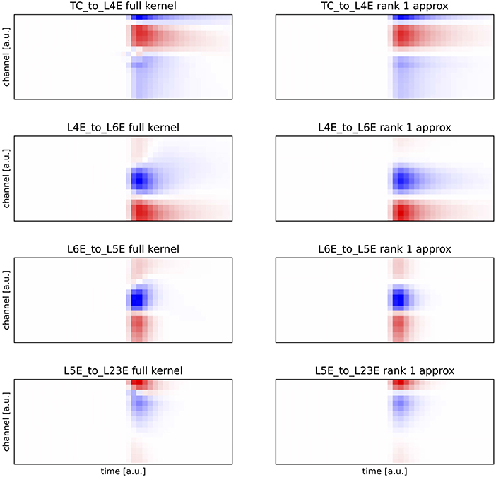
FIGURE A1. Comparison of the full kernels (left side) and their rank 1 approximation (right side). Plots have equal scale.
This is shown more systematically in Figure A2. This plot shows the variance explained for all kernels that have been computed for the cat cortex model [31], that is all combinations from the four layers, both excititory and inhibitory [(4+4)2 kernels] as well as talamic connections to this layers (8). More than 90% of those kernels can be approximated with more than 90% variance explained by a rank 1 approximation.
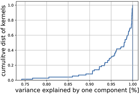
FIGURE A2. The plot shows the variance explained by a rank 1 approximation for all kernels that have been computed form the cat cortex model [31].
Non-linear Case: Analysis Using CP With Non-negativity Constraints
Figure A3 demonstrates the temporal components captured by the CP model with non-negativity constraints. Here, LFP tensors are generated using different strength of non-linearity (β), and analyzed using CP models with non-negativity constraints in the time and trial mode.
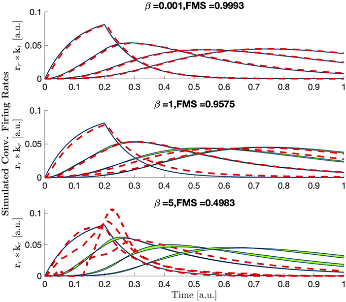
FIGURE A3. Same as Figure 7, but with bounded CP to positive values in the firing rate and trial components. Note that for small non-linearities, the temporal components are almost identical for constrained and unconstrained CP, while for strong non-linearities, where CP fails, the components are very different.
Keywords: tensor decompositions, neuroscience, local field potential (LFP), population rate model, CANDECOMP/PARAFAC, independent component analysis (ICA), principal component analysis (PCA)
Citation: Geddes J, Einevoll GT, Acar E and Stasik AJ (2020) Multi-Linear Population Analysis (MLPA) of LFP Data Using Tensor Decompositions. Front. Appl. Math. Stat. 6:41. doi: 10.3389/fams.2020.00041
Received: 22 June 2020; Accepted: 31 July 2020;
Published: 08 September 2020.
Edited by:
Axel Hutt, Inria Nancy - Grand-Est Research Centre, FranceReviewed by:
Meysam Hashemi, INSERM U1106 Institut de Neurosciences des Systèmes, FrancePeter beim Graben, Brandenburg University of Technology Cottbus-Senftenberg, Germany
Copyright © 2020 Geddes, Einevoll, Acar and Stasik. This is an open-access article distributed under the terms of the Creative Commons Attribution License (CC BY). The use, distribution or reproduction in other forums is permitted, provided the original author(s) and the copyright owner(s) are credited and that the original publication in this journal is cited, in accordance with accepted academic practice. No use, distribution or reproduction is permitted which does not comply with these terms.
*Correspondence: Alexander J. Stasik, YS5qLnN0YXNpa0BmeXMudWlvLm5v
 Justen Geddes
 Gaute T. Einevoll
 Evrim Acar
 Alexander J. Stasik