Non-local Observations and Information Transfer in Data Assimilation

Non-local observations are observations that cannot be allocated one specific spatial location. Examples are observations that are spatial averages of linear or non-linear functions of system variables. In conventional data assimilation, such as (ensemble) Kalman Filters and variational methods information transfer between observations and model variables is governed by covariance matrices that are either preset or determined from the dynamical evolution of the system. In many science fields the covariance structures have limited spatial extent, and this paper discusses what happens when this spatial extent is smaller then the support of the observation operator that maps state space to observations space. It is shown that information is carried beyond the physical information in the prior covariance structures by the non-local observational constraints, building an information bridge (or information channel) that has not been studied before: the posterior covariance can have non-zero covariance structures where the prior has a covariance of zero. It is shown that in standard data-assimilation techniques that enforce a covariance structure and limit information transfer to that structure the order in which local and non-local observations are assimilated can have a large influence on the analysis. Local observations should be assimilated first. This relates directly to localization used in Ensemble Kalman Filters and Smoothers, but also to variational methods with a prescribed covariance structure where observations are assimilated in batches. This suggests that the emphasis on covariance modeling should shift away from the prior covariance and toward the modeling of the covariances between model and observation space. Furthermore, it is shown that local observations with non-locally correlated observation errors behave in the same way as uncorrelated observations that are non-local. Several theoretical results are illustrated with simple numerical examples. The significance of the information bridge provided by non-local observations is highlighted further through discussions of temporally non-local observations, and new ideas on targeted observations.

1. Introduction

The most general form of data assimilation is given by Bayes Theorem that describes how the probability density function (pdf) of the state of the system x is updated when observations y become available:

$\begin{array}{ll}p(\text{x}|\text{y})=\frac{p(\text{y}|\text{x})}{p(\text{y})}p(\text{x})& (1)\end{array}$

in which p(x) is the prior pdf of the state, and p(y|x) the likelihood of the observation given that the state is equal to x. This likelihood is determined by the measurement process. For instance, when the measurement error is additive we can write

$\begin{array}{ll}\text{y}=H(\text{x})+ϵ& (2)\end{array}$

This equation maps the given state vector x into observation space via the observation operator H(..). Since y is given also this equation determines ϵ, and since the pdf of the observation errors is known we know what the likelihood looks like. It is emphasized that Bayes Theorem is a point-wise equation for every possible state vector x.

A non-local observation is typically defined as an observation that cannot be attributed to one model grid point. The consequence is that model state space and observation space should be treated differently. However, Bayes Theorem is still valid, and general enough to tells us how to assimilate these non-local observations.

This is different in practical data-assimilation methods for high-dimensional systems that are governed by local dynamics. Examples are Ensemble Kalman Filters, in which a small number, typically O(10 − 100), of ensemble members is used to mimic a Kalman Filter. Because of the small ensemble size the sample covariance matrix is noisy, and a technique called localization is used to set long-range correlations to zero, as they physically should be, see [1, 2].

Non-local observations can have a support that is larger than the localization area. With support is meant that part of state space that is needed to specify the model equivalent of an observation. When H is linear it is that part of state space that is not mapped to zero. A larger support is not necessarily a problem as long as non-local observations are allowed to influence those model variables with whom they have strong correlations, see e.g., [3]. Assimilating non-local observations as local ones, e.g., by using the grid points where they have most influence, can lead to degradation of the data-assimilation result, as Liu et al. [4] show and hence it is important to retain their full non-local structure.

There has been an extensive search for efficient covariance localization methods that allow for non-local observations, including using off-line climatological ensembles, groups of ensembles, and augmented ensembles in which the ensemble members are localized by construction, see e.g., [5–9].

All of these methods try to find the best possible localization function based on the prior. The main focus of this paper is not on developing better covariance estimates, but rather on the influence on the data-assimilation results of non-local observations in which the support of the observation operator is larger than the dependency (or, for linear relations, correlation) length scale in the prior. This can be due to a mis-specification of the prior localization area, or due to a real prior covariance influence area that is smaller than the support of the observation operator. Since the prior is expected to contain the physical dependencies in the system, this means that a non-local observation needs information from model variables that are physically independent. As will be shown after assimilation new dependencies between the variables involved in the observation operator are generated, on top of the physical dependencies already present. Hence, the non-local observations generate information bridges that are not present in the prior. These bridges can appear both in space and in time.

As an example of the influence of non-local observations on practical data-assimilation systems, since non-local observations generate information bridges, so build new covariance structures, the order in which observations are assimilated becomes important in serial assimilation when covariance length scales are imposed, as in standard localization techniques and in variational methods. This is also true for local observations, but the effect in the non-local case is much larger.

In this paper we will discuss the implications of these information bridges, and strategies of how to assimilate non-local observations. Furthermore, the connection is made to correlated observation errors where the correlations are non-local in the sense defined above. Finally, we discuss ways how we can exploit the appearance of these information bridges to improve data-assimilation systems.

2. The Assimilation of Non-local Observations

In the following we will first demonstrate the treatment of non-local observations in the most general way, via Bayes Theorem, and how non-local observations generate information bridges in the posterior. Then we show that the order in which local and non-local observations are assimilated does not matter, when we solve the full data-assimilation problem, so building the bridges first or later is not relevant. This conclusions does not hold necessarily when approximations to the full data-assimilation problem are introduced, as we will see in later sections.

2.1. Non-local Observations in Bayes Theorem

Let us first study how these information bridges are formed via a simple example. Assume two parts of the state space are independent under the prior, so p(x₁, x₂) = p(x₁)p(x₂), and we have an observation that combines the two, e.g., y = H(x₁, x₂, ϵ), where the observation operator H(..) can be a non-linear function of its arguments. Bayes Theorem shows:

$\begin{array}{ll}p({\text{x}}_1,{\text{x}}_2|y)=\frac{p(y|{\text{x}}_1,{\text{ x}}_2)}{p(y)}p({\text{x}}_1,{\text{x}}_2)=\frac{p(y|{\text{x}}_1,{\text{ x}}_2)}{p(y)}p({\text{x}}_1)p({\text{x}}_2)& (3)\end{array}$

Since y depends on both x₁ and x₂ the likelihood cannot be separated in a function of x₁ only times a function of x₂ only. This means that we also cannot separate the posterior pdf in this way, and hence x₁ and x₂ have become dependent under the posterior. Since Bayes Theorem is the basis of all data-assimilation schemes, the same is true for (Ensemble) Kalman Filters/Smoothers, variational methods, or e.g., Particle Filters.

As an example, Figure 1 shows the joint prior pdf of two independent variables. The pdf is constructed from p(x₁, x₂) = p(x₁)p(x₂) in which p(x₁) is bimodal and p(x₂) a unimodal Gaussian. The likelihood is given in Figure 2, related to an observation y = x₁ + x₂ + ϵ in which ϵ is Gaussian distributed with zero mean. Their product is the posterior given in Figure 3. It is clearly visible that the two variables are highly dependent under the posterior, purely due to the non-local observation.

FIGURE 1

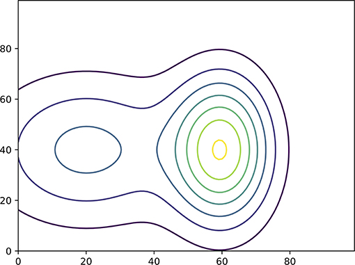
Figure 1. The prior pdf of two independent variables.

FIGURE 2

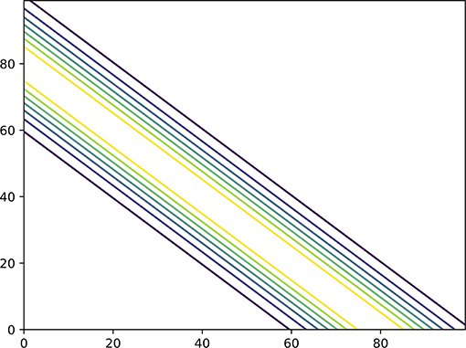
Figure 2. The likelihood as function of the state, corresponding to an observation that is the sum of the two variables. Note that the likelihood is ambiguous on which values of x₁ and x₂ are most likely as the observation only gives the value of a linear combination of them.

FIGURE 3

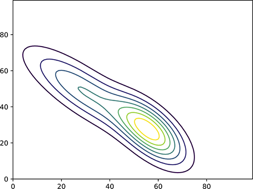
Figure 3. The posterior pdf. Note that the two variables are highly correlated due to the non-local observation.

We now analyse the following simple system in more detail to understand what the influence of non-local spatial observations in linear and linearized data-assimilation methods is. The state is two-dimensional $\text{x}={(x_1,x_2)}^T$, with diagonal prior covariance matrix B with diagonal elements (b₁₁, b₂₂) and a non-local observation operator H = (1 1). A scalar non-local observation y = Hx_true + ϵ_true with measurement error variance r is taken. The subscript true reminds us that the observation is from the true system, while x denotes the state of our model of the real world (this can easily be generalized to different parts x₁ and x₂ of a larger state vector and more, or more complicated, non-local observations y. The two-dimensional system is chosen here for ease of presentation).

The Kalman filter update equation for this system reads:

$\begin{array}{ll}{\text{x}}^a={\text{x}}^b+\text{B}{\text{H}}^T{(\text{H}\text{B}{\text{H}}^T+r)}^{-1}(y-x_1^b-x_2^b)& (4)\end{array}$

with posterior covariance matrix:

$\begin{array}{ll}\text{P}=\left(\begin{array}{cc}{p}_{11}& p_{12}\\ p_{21}& p_{22}\end{array}\right)=\left(\begin{array}{cc}{b}_{11}-b_{11}{b}_{11}/d& -b_{11}{b}_{22}/d\\ -b_{11}{b}_{22}/d& b_{22}-b_{22}{b}_{22}/d\end{array}\right)& (5)\end{array}$

in which d = b₁₁ + b₂₂ + r.

This simple example illustrates the two points from the general case above. Firstly, even if the prior variables are uncorrelated they are correlated in the posterior because of the non-local observation operator mixes the uncorrelated variables of the prior. A second point is that the update of each variable is dependent on the value of the other, even when the two variables are uncorrelated in the prior. Hence the non-local observation acts as an information bridge between uncorrelated variables, both in terms of mean and covariance.

This conclusion remains valid for variational methods like 3DVar as 3DVar implicitly applies the Kalman Filter equations in an iterative manner.

2.2. Order of Observations

The results from the previous section might suggest that the order in which local and non-local observations are assimilated is important: if a non-local observation is assimilated first the next local observation can influence all variables involved in the non-local observation operator. On the other hand, when the local observation is assimilated first this advantage seems to be lost. However, this is not the case, the order in which we assimilate observations is irrelevant in the full Bayesian setting (this is different when localization is used, as explained in section 4).

The easiest way to see this is via Bayes Theorem. Suppose we have two observations, a non-local observation y_nl and a local observation y_l of only x₂. We assume their measurement errors are independent. Bayes Theorem tells us:

$\begin{array}{ll}p(\text{x}|y_l,y_{nl})=\frac{p(y_l,{\mathrm{ y}}_{nl}|\text{x})}{p(y_l,{\mathrm{ y}}_{nl})}p(\text{x})=\frac{p(y_l|x_2)}{p(y_l)}\frac{p(y_{nl}|\text{x})}{p(y_{nl})}p(\text{x})& (6)\end{array}$

If we assimilate y_l first we get:

$\begin{array}{ll}p(\text{x}|y_l,y_{nl})=\frac{p(y_{nl}|\text{x})}{p(y_{nl})}p(\text{x}|y_l)& (7)\end{array}$

and vice versa:

$\begin{array}{ll}p(\text{x}|y_l,y_{nl})=\frac{p(y_l|x_2)}{p(y_l)}p(\text{x}|y_{nl})& (8)\end{array}$

but the result is the same as the order in a multiplication doesn't matter (this is true in theory, in practice differences may arise due to round-off errors). Since the Kalman Filter/Smoother is a special case of this when all pdf's are Gaussian it is true also for the Kalman Filter/Smoother, and for variational methods. As we will see in a later section, care has to be taken when observations are assimilated sequentially and localization is enforced.

To complete the intuition for the Kalman Filter, if the local observation y_l is assimilated first the mean and covariance of variable x₂ are updated, but x₁ remains unchanged. Hence when the non-local observation is assimilated both the mean and covariance of x₂ have changed, and these changed values are used when assimilating the non-local observation, so that x₁ does feel the influence of the local observation via the updated x₂ and its updated variance. Typically the updated x₂ will be such that x₁ + x₂ is closer to y_nl, and its prior covariance before assimilating y_nl will be smaller. The result is that x₁ will be updated stronger than in the case when x₂ has not seen y_l first, as proven in the next section.

3. Kalman Filter/Smoother With Temporally Non-local Observations

The above discussed spatially non-local observations. However, we can easily extend this to temporally non-local observations as we show here in a simple example that illustrates the point. We can easily generalize the results below to the vector case.

We study a one-dimensional system with states xⁿ at time n and an observation y = x^m + xⁿ + ϵ. This problem can be solved by considering a Kalman Smoother, exploring the cross covariance of the states at time n and m, and is explored in standard textbooks. The interesting case is when this prior cross covariance between time n and m is zero, or negligible (for many systems this would mean that m >> n).

Similarly to the spatially non-local case we define the state vector x = (x^m, xⁿ)^T. The prior covariance of this vector depends on the model that governs the evolution of the state in absence of observations. As mentioned, we will study the case that the cross covariance between these two times is zero in the prior, so the prior covariance for this state vector x is given by

$\begin{array}{ll}\text{B}=\left(\begin{array}{cc}{b}_{mm}& 0\\ 0& b_{nn}\end{array}\right)& (9)\end{array}$

The Kalman Filter update equation reads for this case:

$\begin{array}{l}{\text{x}}^a={\text{x}}^b+B{H}^T{\left(HB{H}^T+r\right)}^{-1}(y-H{x}^b)\\ ={\text{x}}^b+B{H}^T{\left(HB{H}^T+r\right)}^{-1}(y-(x^m+x^n))& (10)\end{array}$

with posterior covariance matrix:

$\begin{array}{ll}\text{P}=\left(\begin{array}{cc}{b}_{mm}-b_{mm}{b}_{mm}/d& -b_{mm}{b}_{nn}/d\\ -b_{mm}{b}_{nn}/d& b_{nn}-b_{nn}{b}_{nn}/d\end{array}\right)& (11)\end{array}$

with d = b_mm + b_nn + r.

The similarity with the spatial non-local observations is striking, and indeed the cases are completely identical, with time taking the place of space. The same conclusions as for the spatial case hold: even when states at different times are completely uncorrelated in time under the prior they can be correlated under the posterior when the observation is related to a function of the state vectors at both times, providing an information bridge between the two times.

4. Consequences for Sequential Updating Schemes With Fixed Covariance Length Scales

The results above show that when non-local observations are assimilated they significantly change the prior covariance length and/or time-scales during the data-assimilation process. This has direct consequences for methods that assimilate observations sequentially and at the same time enforce covariance structures with certain length scales. An example is a Local Ensemble Kalman Filter, in which spurious correlations are suppressed either by Schur-multiplying the prior ensemble covariance with a local correlation matrix or Schur-multiplying the inverse of the observation error covariance matrix with a distance function. This procedure effectively sets covariances equal to zero above a certain distance between grid points. This localization in combination with sequential observation updating has to be done with care, as shown below. Another example is a 3D or 4DVar in which observations are assimilated in batches.

Assimilation of non-local observations that span length scales larger than the localization correlation length scale can potentially lead to suboptimal updates if the observations are assimilated in the wrong order. This is illustrated below, first theoretically and then with a simple example.

4.1. The Influence of Localization

Let us assume we have two variables x₁ and x₂ that lie outside each others localization area. A localization area is defined here as the area in which observations are allowed to influence the grid point in consideration. Two observations are made, a non-local observation y₁ = x₁ + x₂ + ϵ₁ and a local observation y₂ = x₂ + ϵ₂. We study the result of the data-assimilation process on variable x₁ where we change the order of assimilation.

When we assimilate the non-local observation y₁ first, we find the update:

$\begin{array}{ll}{\widehat{x}}_1=x_1+\frac{b_{11}}{b_{11}+b_{22}+r_1}(y_1-(x_1+x_2))& (12)\end{array}$

$\begin{array}{ll}{\widehat{b}}_{11}=b_{11}-\frac{b_{11}^2}{b_{11}+b_{22}+r_1}& (13)\end{array}$

As shown in the previous sections, this assimilation generates a cross covariance between x₁ and x₂ as

$\begin{array}{ll}{\widehat{b}}_{12}=-\frac{b_{11}{b}_{22}}{b_{11}+b_{22}+r_1}& (14)\end{array}$

When we now assimilate observation y₂ the fixed covariance length scale, from localization or otherwise, we will remove the cross covariance ${\widehat{b}}_{12}$ before y₂ is assimilated, and hence x₁ is not updated further, so $x_1^a={\widehat{x}}_1$ and $b_{11}^a={\widehat{b}}_{11}$ and $b_{12}^a=0$.

The story is different when we first assimilate y₂ and then y₁. In this case we find that x₁ is not updated by y₂, but x₂ and its variance are. Let's denote these updated variables by ${\widehat{x}}_2$ and ${\widehat{b}}_{22}$. We then find for the update of x₁ by the non-local observation y₁:

$\begin{array}{ll}{x}_1^a=x_1+\frac{b_{11}}{b_{11}+{\widehat{b}}_{22}+r_1}(y_1-(x_1+{\widehat{x}}_2))& (15)\end{array}$

$\begin{array}{ll}{b}_{11}^a=b_{11}-\frac{b_{11}^2}{b_{11}+{\widehat{b}}_{22}+r_1}& (16)\end{array}$

$\begin{array}{ll}{b}_{12}^a=-\frac{b_{11}{\widehat{b}}_{22}}{b_{11}+{\widehat{b}}_{22}+r_1}& (17)\end{array}$

We can now substitute the ˆ values in these expressions. We start with the posterior variance $b_{11}^a$. We find, after some algebra:

$\begin{array}{ll}{b}_{11}^a=b_{11}-\frac{b_{11}^2}{b_{11}+b_{22}+r_1}(1+d)& (18)\end{array}$

in which $d=b_{22}^2/\left[(b_{22}+r_2)(b_{11}+b_{22}+r_1)-b_{22}^2\right]$. The first and second terms in the expression above appear when we would assimilate y₁ first, and the third term proportional to d is an extra reduction of the variance of x₁ due to the fact that we first assimilated y₂. That reduction is absent when we first assimilate y₁ and then assimilate y₂ due to the localization procedure as shown above.

This third term can be as large as the second term. We can quantify this with the following example, in which we assume the prior variances of x₁ and x₂ are the same, hence b₂₂ = b₁₁ = b. In that case d becomes $\widehat{d}$ defined by:

$\begin{array}{ll}\widehat{d}=\frac{1}{(2+r_1/b)(1+r_2/b)-1}& (19)\end{array}$

This is the extra reduction due to assimilating y₁ after y₂, relative to the reduction due to assimilating y₁ alone. In Figure 4 the size of this term is shown as function of r₁/b and r₂/b. As expected the size increases when the observation errors are smaller than the prior variances.

FIGURE 4

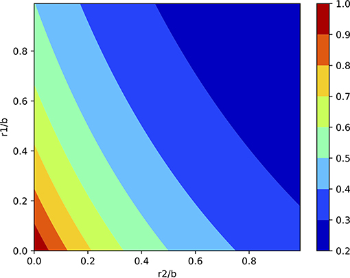
Figure 4. Extra reduction of the posterior variance when the non-local observation is assimilated after the local observations compared to assimilating the observations the other way around (the factor $\widehat{d}$ in Equation 19). This is purely due to the fixed covariance length scales used in the prior.

Let us now look at the posterior mean, for which we find:

$\begin{array}{l}{x}_1^a=x_1+\frac{b_{11}}{b_{11}+b_{22}+r_1}(y_1-(x_1+x_2))\\ -\frac{b_{11}}{b_{11}+b_{22}+r_1}\frac{b_{22}}{b_{22}+r_2}(y_2-x_2)\\ +\frac{d{b}_{11}}{b_{11}+b_{22}+r_1}((y_1-(x_1+x_2))\\ -\frac{b_{22}}{b_{22}+r_2}(y_2-x_2))& (20)\end{array}$

The first line is the contribution purely from the non-local observation. It appears when we first assimilate the non-local observation and then the local observation, and is equal to Equation (12). However, first assimilating y₂ and then the non-local observation y₁ leads to the appearance of two extra terms. The term related to y₂ − x₂ is a direct contribution of the innovation of the local observation at x₂ (as can be seen from ${\widehat{x}}_2=x_2+b_{22}/(b_{22}+r)(y_2-x_2)$), and can be traced back to the fact that x₂ has changed due to assimilation of y₂ first. The other term is related to the change in the variance of x₂ due to the assimilation of y₂.

To understand the importance of these two extra terms we again assume b₁₁ = b₂₂ = b, to find:

$\begin{array}{l}{x}_1^a=x_1+\frac{1}{2+r_1/b}[(y_1-(x_1+x_2))-\frac{1}{1+r_2/b}(y_2-x_2)\\ +d\left((y_1-(x_1+x_2))-\frac{1}{1+r_2/b}(y_2-x_2)\right)]& (21)\end{array}$

where d = 1/[(2 + r₁/b)(1 + r₂/b) − 1]. Of course, the value of $x_1^a$ depends on the actual values for the observations and the prior means. To obtain an order of magnitude estimate we assume that the innovation y₁ − (x₁ + x₂) is of order $\sqrt{2b+r_1}$. and similarly $y_2-x_2\approx \sqrt{b+r_2}$. Since the signs of the different contributions depend on the actual signs of y₁ − (x₁ + x₂) and y₂ − x₂ we proceed as follows. We rewrite the expression for $x_1^a$ as:

$\begin{array}{l}{x}_1^a=x_1+\frac{1}{2+r_1/b}[(y_1-(x_1+x_2))(1+d)\\ -\frac{1}{1+r_2/b}(y_2-x_2)(1+d)]& (22)\end{array}$

Hence the ratio of the first extra term d(y₁ − (x₁ + x₂)) to the contribution only from y₁ is proportional to d, and is given in Figure 4. The ratio of the rest to the contribution only from y₁ is given in Figure 5. Note that we used the approximations for y₂ − x₂ and y₁ − (x₁ + x₂) above, which means that this ratio becomes

$\begin{array}{ll}\frac{1+d}{\sqrt{(1+r_2/b)(2+r_1/b)}}& (23)\end{array}$

The sign of this contribution is unclear, as mentioned above, so we have to either add to or subtract this figure from Figure 4.

FIGURE 5

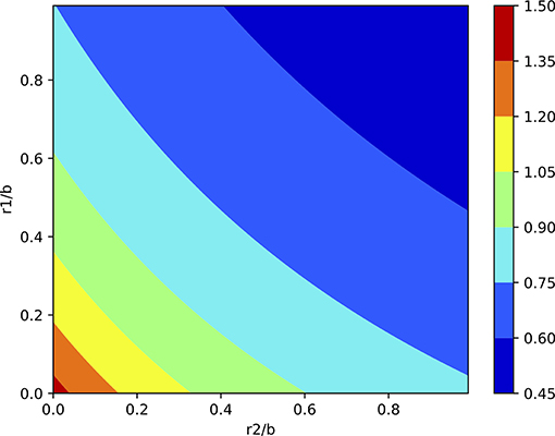
Figure 5. Second contribution of assimilation local observation y₂ first, as given as the ratio in Equation (23). This figure should be added to or subtracted from Figure 4.

The importance of Figures 4, 5 is that they show that when the observation errors are small compared to the prior variance the update could be more than 100% too small when localization is used if one first assimilates the non-local observation y₁, followed by assimilating y₂. Hence non-local observations should be assimilated after local observations.

When the update is not sequential, but instead local and non-local observations are assimilated in one go, we obtain the same result we would obtain by first assimilating the local observation and then the non-local observation. The reason is simple: assimilating the non-local observation means that all grid points in the domain of the non-local observation are allowed to see all other gridpoints in that domain, and hence information from local observations is shared too.

It is emphasized again that the above conclusions are not restricted to Ensemble Kalman Filters and Smoothers. Any scheme that assimilates observations sequentially, or in batches, should ensure that non-local observations in which the support of the observation operator is larger than the correlation length scales used in the covariance models should be assimilated after the local observations.

4.2. An Assimilation Example

To illustrate the effect explained in the previous section the following numerical experiment is conducted. We run a 40-dimensional model, the Lorenz 1996 model, with an evolution equation for each state component given by:

$\begin{array}{ll}\frac{d{x}_i}{dt}=(x_{i+1}-x_{i-2})x_{i-1}-x_i+F+{\beta }_i& (24)\end{array}$

The forcing F = 8 is a standard value ensuring chaotic dynamics. The system is periodic. We use a Runge-Kutta 4 scheme with time step Δt = 0.01. The β_i are random variables denoting model errors, white in time and β_i ~ N(0, Q) in space, in which Q^1/2 is a tridiagonal matrix with 0.1 on the diagonal and 0.025 on the subdiagonals.

The model is spun up from a random state in which each $x_i~N(0,10^{-4})$, is independent from the other state components. The spin up time is 10,000 time steps. Then a true model evolution is generated for 10,000 time steps, starting at time zero. Observations are created from this true run every Δt_obs time steps, with observation errors drawn from N(0, R) in which R is diagonal. Both Δt_obs and R are varied in the experiments below. Local observations are taken from positions [5, 10, 15, 20, 25, 30, 35] and a non-local observation is taken as Hx = x₀ + x₅.

An LETKF is used with a Gaspari-Cohn localization function on R⁻¹ with cut-off radius of 5 gridpoints, which means that observation error variances are multiplied by a factor >10 after 3 grid points, so they have little influence compared to observations close to the updated grid point. This localization is kept constant to illustrate the effects; it might be tuned in real situations. The ensemble consist of 10 members, initialized from the true state at time zero with random perturbations drawn from N(0, I). When assimilating the non-local observation the localization is only applied outside the domain of the non-local observation.

We run two sets of experiments, one set in which all the local observations are assimilated first at an analysis time, followed by assimilating the non-local observation, and one in which the non-local observation is assimilated first, followed by all other observations. We looked at the difference of these two assimilation runs for different values of the observation period Δt_obs and different values of the observation error variances in R. All observation error values for local and non-local observations are the same.

Figure 6 shows the posterior RMSE averaged over all assimilation times of the state component x₀ as function of the chosen observation error standard deviation. The different lines correspond to the different observation periods, ranging from 10, via 20 to 50 time steps, in colors black, blue, and red, respectively. The solid lines denote the results when the non-local observation is assimilated last, and the dashed lines show results when the non-local observation is assimilated first. All results are averaged over 10 model runs, and the resulting uncertainty is of the order of 0.1. Increasing the average to 100 model runs did not differ the numbers within these error bounds.

FIGURE 6

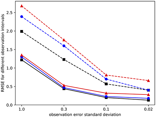
Figure 6. RMSE of state component x₀ which is part of a non-local observation, as function of observation error. The black (squares), blue (dots), and red (triangles) lines denote observation periods of 10, 20, and 50 time steps. The solid lines are for cases in which the non-local observation is assimilated last, dashed lines when non-local observation is assimilated first. Note the logarithmic horizontal scale. The figure shows that assimilating the non-local observation after local observations is beneficial.

As can be seen from the figure, assimilating the non-local observation last leads to a systematically lower RMSE for all observation periods and for all observation error sizes. These results confirm the theory in the previous section.

We also performed several experiments in which the observation error in the non-local observation was higher or lower than that in the local observations for the experiment with Δt_obs = 20 time steps. As an example of the results, increasing the non-local observation error from 0.1 to 0.3 increased the RMSE in x₀ from 0.23 to 0.24 when the non-local observation is assimilated last, but from 0.70 to 0.81 when it is assimilated first. This shows that the impact of a larger non-local observation error is less when the non-local observation is assimilated last because of the benefit of the more accurate state x₅. When the non-local observation is assimilated first this update of x₅ is not noticed by the data-assimilation system.

In another example we decreased the observation error of the non-local observation from 0.3 to 0.1. In this case the RMSE of x₀ remained at 0.47 when the non-local observation is assimilated last, and decreased from 1.60 to 1.50 when it is assimilated first. As expected, the influence is much smaller in the former case as the state at x₅ is now less accurate. Hence, also these experiments demonstrate that the theory developed above is useful.

Finally, the results are independent of the dimension of the system; a 1,000-dimensional Lorenz 1996 model yields results that are very similar and with differences smaller than the uncertainty estimate of 0.1. This is because the analysis is local, and the non-local observation spans just part of the state space.

5. Correlated Observation Errors

Although observations errors are typically assumed to be uncorrelated in data-assimilation systems, they in fact are often correlated, and the correlation length scales can even be longer than the correlation length scales in the prior. Correlated observation errors can either arise from the measurement instrument, e.g., via correlated electrical noise in satellite observations, but also from the mismatch between what the observations and the model represent. The latter are called representation errors and typically arise when the observations have smaller length scales than the model can resolve. See e.g., full explanations of representation errors in Hodyss and Nichols [10] and Van Leeuwen [11], and a recent review by Janjić et al. [12].

The latter, representation errors, typically do not lead to non-local correlation structures in the model domain as the origin of these errors is sub grid scale. The discussion here focusses on correlation between observation errors of observations that are farther apart than the localization radius or than the imposed correlation length scales in variational methods. As we will see, there is a strong connection to non-local observations.

5.1. A Simple Example

Let us look at a simple example of two grid points that are farther apart than the imposed localization radius, or than physical correlation length scales. Both are observed, and the observation errors of these two observations are correlated. The observation operator H = I, the identity matrix. The covariance matrices read:

$\begin{array}{ll}\text{B}=\left(\begin{array}{cc}{b}_{11}& 0\\ 0& b_{22}\end{array}\right)\text{ and }\text{R}=\left(\begin{array}{cc}{r}_{11}& r_{12}\\ r_{21}& r_{22}\end{array}\right)& (25)\end{array}$

The inverse in the Kalman gain is a full matrix:

$\begin{array}{ll}{\left(\text{H}\text{B}{\text{H}}^T+\text{R}\right)}^{-1}=\frac{1}{D}\left(\begin{array}{cc}{b}_{22}+r_{22}& -r_{12}\\ -r_{21}& b_{11}+r_{11}\end{array}\right)& (26)\end{array}$

in which D is the absolute value of the determinant, given by D = (b₁₁ + r₁₁)(b₂₂ + r₂₂) − r₁₂r₂₁. The factor BH^T is diagonal, as H is the identity matrix. Because of the non-zero off-diagonal elements in the resulting Kalman gain the state component x₁ is updated as:

$\begin{array}{ll}{x}_1^a=x_1^b+\frac{1}{D}{b}_{11}(b_{22}+r_{22})(y_1-x_1)-\frac{1}{D}{b}_{11}{r}_{12}(y_2-x_2)& (27)\end{array}$

To make sense of this equation we rewrite it, after some algebra, as:

$\begin{array}{ll}{x}_1^a=x_1^b+\frac{b_{11}}{b_{11}+r_{11}}\left[(y_1-x_1)+\frac{{\rho }_1{\rho }_2(y_1-x_1)-{\rho }_2(y_2-x_2)}{1-{\rho }_1{\rho }_2}\right]& (28)\end{array}$

in which

$\begin{array}{ll}{\rho }_1=\frac{r_{12}}{b_{11}+r_{11}}\text{ and }{\rho }_2=\frac{r_{12}}{b_{22}+r_{22}}& (29)\end{array}$

This equation shows us several interesting phenomena. The first term in the brackets denotes the update of x₁ when we would only use observation y₁. The other term has to do with using observation y₂ while its errors are correlated with that of y₁. Interestingly, the update by y₁ gets enhanced by a term with factor ρ₁ρ₂/(1 − ρ₁ρ₂), which is positive. This update is also changed by y₂, with a sign depending on r₁₂ and y₂ − x₂. To understand where these terms come from we can rewrite the expression above further as:

$\begin{array}{ll}{x}_1^a=x_1^b+\frac{b_{11}}{b_{11}+r_{11}}\left[\frac{1}{1-{\rho }_1{\rho }_2}(y_1-x_1)-\frac{{\rho }_2}{1-{\rho }_1{\rho }_2}(y_2-x_2)\right]& (30)\end{array}$

We now see that the influence of the correlated observation errors is to change the denominator of the factor that multiplies the innovation y₁ − x₁. That denominator becomes smaller because of the cross correlations, so the innovation will lead to a larger update.

The influence of the second innovation is not that straightforward. Let's take the situation that the errors in the two observations are positively correlated, so ρ₂ > 0. Now assume that y₁ − x₁ is positive. Then, as expected, the K₁₁ element of the gain is positive, so the update to x₁ is positive. Indeed, we want to move the state closer to the observation y₁. On the other hand, we know that x₁ is an unbiased estimate of the truth, so this does suggest that the realization of the observation error of y₁ is positive. Let's also assume that y₂ − x₂ is positive. As also x₂ is assumed unbiased this suggests that the observation error in y₂ is positive too. The filter knows that these two errors are correlated via the specification of R. Because both innovations indicate that the actual observation error is positive it will incorporate the contribution from y₂ − x₂ with a negative sign to avoid a too large positive update of x₁. If, on the other hand, y₂ − x₂ would have been negative the filter has no indication that the actual observation error positive or negative, so y₂ − x₂ would be allowed to add positively to x₁. However, note that innovation will act negatively on the update of x₂. The Kalman Filter is a clever device, designed to ensure an unbiased posterior for both x₁ and x₂.

A similar story holds for x₂ as the problem is symmetric. This shows that neglecting long-range correlations in observation errors can lead to suboptimal results with analysis errors that are too large. Similar results have been found for locally correlated observations, e.g., [13, 14], and recent discussions on the interplay between HBH^T and R in Miyoshi et al. [15] and Evensen and Eikrem [16].

5.2. The Connection to Non-local Observations

An interesting connection can be made with recent ideas to transform observations such that their errors are uncorrelated. The interest for such a transform stems from the fact that many data-assimilation algorithm implementations either assume uncorrelated observation errors or run much more efficiently when these errors are uncorrelated. Let us assume such a transformation is performed on our two observations. There are infinitely many transformations that do this, and let us assume here that the eigenvectors of R are used.

Decomposing R gives R = UΣU^T in which the columns of U contain the eigenvectors and Σ is a diagonal matrix with on the diagonal the eigenvalues

$\begin{array}{ll}{\lambda }_{1,2}=\frac{1}{2}\left(Tr(\text{R})\pm \sqrt{Tr{(\text{R})}^2-4det\text{R}}\right)& (31)\end{array}$

If we transform the observation vector as $\widehat{\text{y}}={\text{U}}^T\text{y}$ this new vector has covariance matrix Σ, and hence the errors in the components of $\widehat{\text{y}}$ are uncorrelated. The interesting observation is now that the components of $\widehat{\text{y}}$ are non-local observations with uncorrelated errors. Hence, our analysis of the influence of non-local observations applies directly to this case.

As a simple example, assume r₁₁ = r₂₂ = r and r₁₂ = r₂₁ = ρr (this could be worked out for the general case, but the expressions become complicated and serve no specific purpose for this paper). In that case λ_1,2 = r(1 ± ρ) and the eigenvectors are ${(1,1)}^T/\sqrt{2}$ and ${(1,-1)}^T/\sqrt{2}$. This leads to transformed observations ${\widehat{y}}_1=(x_1+x_2)/\sqrt{2}$ and ${\widehat{y}}_2=(x_1-x_2)/\sqrt{2}$.

Using the Kalman Filter update equation for variable x₁ we find:

$\begin{array}{l}{x}_1^a=x_1+\frac{1}{\sqrt{2}D}[b_{11}(b_{22}+{\lambda }_2)\left({\widehat{y}}_1-\frac{1}{\sqrt{2}}(x_1+x_2)\right)\\ +b_{11}(b_{22}+{\lambda }_1)\left({\widehat{y}}_2-\frac{1}{\sqrt{2}}(x_1-x_2)\right)]& (32)\end{array}$

in which $D=\left[\left(b_{11}+b_{22}+2{\lambda }_1\right)\left(b_{11}+b_{22}+2{\lambda }_2\right)-{\left(b_{11}+b_{22}\right)}^2\right]/4$ which turns out to be the same D as found for the correlated observation errors. This is not surprising as with y also H and R have been transformed, and hence HBH^T + R has transformed in the same way. This means we can always extract a similar factor from the denominator of the Kalman update. Hence, we have transformed the problem from local observations with non-locally correlated errors to non-local observations with uncorrelated errors.

To show that this is the same as the original problems we now rewrite this analysis for the observations with correlated errors, so in terms of y, and collect terms y₁ − x₁ and y₂ − x₂ to find:

$\begin{array}{ll}{x}_1^a=x_1+\frac{1}{D}{b}_{11}(b_{22}+r)(y_1-x_1)-\frac{1}{D}{b}_{11}\rho r(y_2-x_2)& (33)\end{array}$

With r₂₂ = r and r₁₂ = ρr we recover the analysis equation for the correlated observation error case.

Hence we have shown that assimilating correlated observations with correlation length scales larger than physical length scales is the same as assimilating the corresponding non-local uncorrelated observations (this result has resemblance to but is different from that of Nadeem and Potthast [17], who discuss transforming all observations, local and non-local such that they all become local observations. They then do the localization and data assimilation in this space, and transform back to physical space. This, of course, will lead to correlated errors in the transformed non-local observations).

It will not come as a surprise that if observations are assimilated sequentially and localization, or a fixed covariance length scale, is used the order of assimilation matters, and non-locally correlated observations should be assimilated after local observations. Finally, it is mentioned that the story is similar for non-local observation error correlations in time.

6. Exploiting Non-local Observations

As mentioned above, to avoid cutting off non-local observation information during sequential assimilation it is best to assimilate the non-local observation after the local observations. However, an alternative strategy is to change the localization area if that is possible. Before the non-local observation is assimilated the localization area should remain as is. As soon as the non-local observation is assimilated we have created significant non-zero correlations along the domain of the non-local observation operator. This means that we can include this area in the localization domain.

To illustrate this idea the same experiments from section 4 have been repeated applying the procedure outlined above for Δt_obs = 10, and used the real observation error of the observation at x₅ in location x₀. This means that effectively there is no localization between these two grid points. This is an extreme case, but does illustrate the point we want to make. The results are depicted in Figure 7.

FIGURE 7

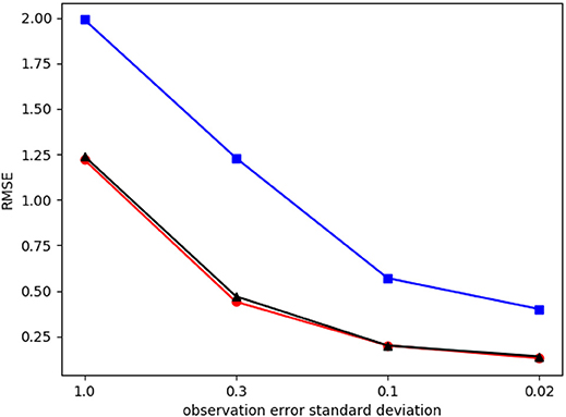
Figure 7. RMSE of state component x₀ which is part of a non-local observation, as function of observation error for Δ_obs = 10. Cases in which the non-local observation is assimilated last (red, dots), when non-local observation is assimilated first (blue, squares), and when the non-local observation is assimilated first and localization area is adapted with localization effectively removed between x₅ and x₀ (black, triangles).

They show that changing the localization area after assimilating the non-local observation does help. In theory, for two variables, this should give the same result as assimilating the non-local observation after the local observation. That this is not the case here is because grid point 5 is also updated slightly by grid point 10, and that reduces the variance at x₁ further when the non-local observation is assimilated last, while that information is not available when the non-local observation is assimilated first. The conclusion is that changing the localization area after assimilating a non-local observation is beneficial for the data-assimilation result.

Another way to explore the features of non-local observations in data assimilation is as follows. Assume we have an area of interest that is poorly observed, and not easily observed locally. We assume that we do not have and cannot obtain accurate local observations in that area, but a non-local observation is possible. Section 4, and specifically Equation (18) shows that is make sense to ensure that the support of this non-local observation contains a well-observed area. In this way the area of interest will benefit from the accurate information from the well-observed area via the information bridge. Another way of phrasing what happens is that by having an accurately observed area in the support of the non-local observation its information is redistributed more toward Another possibility along the same lines is when we already have a non-local observation containing the area of interest in its support. The accuracy in the area of interest can be enhanced by performing extra local observations in an easy to observe area, that is in the support of the non-local observation. Hence again we exploit the information bridge, this time by adding a local observation in a well-chosen position. This idea provides a new way to perform targeted observations that has not been explored as yet, as far as this author knows. This could also be exploited in time, or even in space and time.

Finally, one might think that it is possible to enhance the accuracy of the update in an area of interest by artificially introducing correlated observation errors between observations in that area and observations in another well-observed area. Since correlated observation errors can be transformed to non-local observations a similar information bridge can be build that might be beneficial.

To study this in detail we use the example from section 5.1. Assume that we have two observations with uncorrelated errors, and we add a fully correlated random perturbation with zero mean to them, so y₁ = Hx₁ + ϵ₁ + ϵ and y₂ = Hx₂ + ϵ₂ + ϵ in which ϵ₁ and ϵ₂ are uncorrelated, and ϵ ~ N(0, r), the same value for each observation. Hence this ϵ term contains the fully correlated part of the observation error that we added to the observations artificially. This leads to a correlated observational error covariance given by:

$\begin{array}{ll}\text{R}=\left(\begin{array}{cc}{r}_{11}+r& r\\ r& r_{22}+r\end{array}\right)& (34)\end{array}$

Using this in the Kalman gain we find for the gain of observation y₁:

$\begin{array}{l}\frac{1}{D}{b}_{11}(b_{22}+r_{22}+r)\\ =\frac{b_{11}(b_{22}+r_{22}+r)}{|(b_{11}+r_{11}+r)(b_{22}+r_{22}+r)-r^2|}\\ =\frac{b_{11}}{(b_{11}+r_{11})}\frac{(b_{22}+r_{22}+r)(b_{11}+r_{11})}{|(b_{11}+r_{11}+r)(b_{22}+r_{22}+r)-r^2|}\\ =\frac{b_{11}}{(b_{11}+r_{11})}\frac{(b_{22}+r_{22}+r)(b_{11}+r_{11})}{|(b_{22}+r_{22}+r)(b_{11}+r_{11})+r(b_{22}+r_{22})|}& (35)\end{array}$

The first ratio is the Kalman gain without the correlated observation error contribution. This is multiplied by the factor when the correlated observation error is included. We immediately see that this factor is smaller then 1, so reducing the Kalman gain. This shows that adding extra correlated observation errors to observations that are farther apart then the covariance structures in the prior will not lead to better updates: in fact the updates will deteriorate (As an aside, this would be different if we would have access to ϵ₁ and ϵ₂, in which case ϵ could be a linear combination of these two, and the Kalman gain could be made larger than the gain for just assimilating y₁. Unfortunately, we are given y₁ and y₂, not their error realizations).

7. Conclusions and Discussion

In this paper we studied the information transfer in data-assimilation systems when non-local observations are assimilated. Non-local observations are defined here as observations with a observation operator support that is larger then the covariance length scales. This pertains to both spatial and temporal non-locality. It is found that these observations connect parts of the domain that were not connected in the prior, building an information bridge that is longer than the physics and statistics in the prior predict. Hence the notion that information from observations is spread around via the correlation length scales in B is only part of the story as non-local observations can spread information over larger distances. Indeed, one should look at the full BH^T factor of the gain, and realize that the observation operator can change the covariance structures.This suggests that the emphasis on covariance modeling should shift away from the prior covariance and toward the modeling of the covariances between model and observation space.

We showed how non-local observation information is transferred to the posterior in Bayes Theorem and hence in fully non-linear and in linear and linearized data-assimilation schemes, such as (Ensemble) Kalman Filters and variational methods. Then we elaborated on the interaction of localized covariances, as typically used in the geosciences, and the sequential assimilation of observations. It was shown that it is beneficial to assimilate non-local observations after local observations in order to maximize information flow from observations in the data-assimilation system. This was quantified both analytically and numerically.

Furthermore, it was shown that observations with non-locally correlated observation errors can be transformed to non-local observations with uncorrelated observation errors, demonstrating the equivalence of the two.

In an attempt to explore the information flow by non-local observations we showed that non-local observations do not have to be assimilated after local observations if localization areas are extended along the support of the non-local observation operator after the non-local observations are assimilated, both analytically and with a numerical example.

Furthermore, it was shown that targeted non-local observations can be used to bring the information from accurate observations to other parts of the system. It was also shown that it is not beneficial to add correlated observation errors to distant observations to set up an information bridge as that will always be detrimental.

These initial explorations of non-local observations might guide the development of real data-assimilation applications where observations are assimilated sequentially and non-local observations and/or non-locally correlated observation errors are used. The main message might be that one should not optimize for the covariance structures in the prior, but optimize the covariance structures between observations and model variables.

Data Availability Statement

The datasets generated for this study are available on request to the corresponding author.

Author Contributions

The author confirms being the sole contributor of this work and has approved it for publication.

Funding

The author thanks the European Research Council (ERC) for funding the CUNDA project 694509 under the European Union Horizon 2020 research and innovation programme.

Conflict of Interest

The author declares that the research was conducted in the absence of any commercial or financial relationships that could be construed as a potential conflict of interest.

The handling editor and reviewer AC declared their involvement as co-editors in the Research Topic, and confirm the absence of any other collaboration.

Acknowledgments

I would like to thank the two reviewers for valuable comments that greatly improved the paper.

References

1. Houtekamer PL, Mitchell HL. A sequential ensemble Kalman filter for atmospheric data assimilation. Mon Weather Rev. (2001) 129:123–37. doi: 10.1175/1520-0493(2001)129<0123:ASEKFF>2.0.CO;2

CrossRef Full Text | Google Scholar

2. Hamill TM, Whitaker JS, Snyder C. Distance-dependent filtering of background-error covariance estimates in an ensemble Kalman filter. Mon Weather Rev. (2001) 129:2776–90. doi: 10.1175/1520-0493(2001)129<2776:DDFOBE>2.0.CO;2

CrossRef Full Text | Google Scholar

3. Fertig EJ, Hunt BR, Ott E, Szunyogh I. Assimilating non-local observations with a local ensemble Kalman filter. Tellus A. (2007) 59:719–30. doi: 10.1111/j.1600-0870.2007.00260.x

CrossRef Full Text | Google Scholar

4. Liu H, Anderson JL, Kuo YH, Snyder C, Caya A. Evaluation of a nonlocal quasi-phase observation operator in assimilation of CHAMP radio occultation refractivity with WRF. Mon Weather Rev. (2007) 136:242–56. doi: 10.1175/2007MWR2042.1

CrossRef Full Text | Google Scholar

5. Anderson JL. Exploring the need for localization in ensemble data assimilation using a hierarchical ensemble filter. Phys D. (2007) 230:99–111. doi: 10.1016/j.physd.2006.02.011

CrossRef Full Text | Google Scholar

6. Anderson JL, Lei L. Empirical localization of observation impact in ensemble Kalman filters. Mon Weather Rev. (2013) 141:4140–53. doi: 10.1175/MWR-D-12-00330.1

CrossRef Full Text | Google Scholar

7. Lei L, Anderson JL, Whitaker JS. Localizing the impact of satellite radiance observations using a global group ensemble filter. J Adv Model Earth Syst. (2016) 8:719–34. doi: 10.1002/2016MS000627

CrossRef Full Text | Google Scholar

8. Campbell WF, Bishop CH, Hodyss D. Vertical covariance localization for satellite radiances in ensemble Kalman filters. Mon Weather Rev. (2010) 138:282–90. doi: 10.1175/2009MWR3017.1

CrossRef Full Text | Google Scholar

9. Farchi A, Bocquet M. On the efficiency of covariance localisation of the ensemble Kalman filter using augmented ensembles. Front Appl Math Stat. (2019) 5:3. doi: 10.3389/fams.2019.00003

CrossRef Full Text | Google Scholar

10. Hodyss D, Nichols N. The error of representation: basic understanding. Tellus A. (2015) 67:822. doi: 10.3402/tellusa.v67.24822

CrossRef Full Text | Google Scholar

11. Van Leeuwen PJ. Representation errors and retrievals in linear and nonlinear data assimilation. Q J R Meteorol Soc. (2015) 141:1612–23. doi: 10.1002/qj.2464

CrossRef Full Text | Google Scholar

12. Janjić T, Bormann N, Bocquet M, Carton JA, Cohn SE, Dance SL, et al. On the representation error in data assimilation. Q J R Meteorol Soc. (2018) 144:1257–78. doi: 10.1002/qj.3130

CrossRef Full Text | Google Scholar

13. Garand L, Heilliette S, Buehner M. Interchannel error correlation associated with AIRS radiance observations: inference and impact in data assimilation. J Appl Meteorol Climatol. (2007) 46:714–25. doi: 10.1175/JAM2496.1

CrossRef Full Text | Google Scholar

14. Stewart L, Dance S N, Nichols. Correlated observation errors indata assimilation. Int J Numeric Methods Fluids. (2008) 56:1521–7. doi: 10.1002/fld.1636

CrossRef Full Text | Google Scholar

15. Miyoshi T, Kalnay E, Li H. Estimating and including observation-error correlations in data assimilation. Inverse Probl Sci Eng. (2013) 21:387–98. doi: 10.1080/17415977.2012.712527

CrossRef Full Text | Google Scholar

16. Evensen G, Eikrem KS. Conditioning reservoir models on rate data using ensemble smoothers. Comput Geosci. (2018) 22:1251–70. doi: 10.1007/s10596-018-9750-8

CrossRef Full Text | Google Scholar

17. Nadeem A, Potthast R. Transformed and generalized localization for ensemble methods in data assimilation. Math Methods Appl Sci. (2016) 39:619–34. doi: 10.1002/mma.3496

CrossRef Full Text | Google Scholar