Chimera States in Networks of Locally and Non-locally Coupled SQUIDs

Planar and linear arrays of SQUIDs (superconducting quantum interference devices) operate as non-linear magnetic metamaterials in microwaves. Such SQUID metamaterials are paradigmatic systems that serve as a test-bed for simulating several non-linear dynamics phenomena. SQUIDs are highly non-linear oscillators which are coupled together through magnetic dipole-dipole forces due to their mutual inductance; that coupling falls-off approximately as the inverse cube of their distance, i.e., it is non-local. However, it can be approximated by a local (nearest-neighbor) coupling which in many cases suffices for capturing the essentials of the dynamics of SQUID metamaterials. For either type of coupling, it is numerically demonstrated that chimera states as well as other spatially non-uniform states can be generated in SQUID metamaterials under time-dependent applied magnetic flux for appropriately chosen initial conditions. The mechanism for the emergence of these states is discussed in terms of the multistability property of the individual SQUIDs around their resonance frequency and the attractor crowding effect in systems of coupled non-linear oscillators. Interestingly, controlled generation of chimera states in SQUID metamaterials can be achieved in the presence of a constant (dc) flux gradient with the SQUID metamaterial initially at rest.

1. Introduction

The notion of metamaterials refers to artificially structured media designed to achieve properties not available in natural materials. Originally they were comprising subwavelength resonant elements, such as the celebrated split-ring resonator (SRR). The latter, in its simplest version, is just a highly conducting metallic ring with a slit, that can be regarded as an effectively resistive–inductive–capacitive (RLC) electrical circuit. There has been a tremendous amount of activity in the field of metamaterials the last two decades, the results of which have been summarized in a number of review articles [1–8] and books [9–16]. One of metamaterial's most remarkable properties is that of the negative refraction index, which results from simultaneously negative dielectric permittivity and diamagnetic permeability.

An important subclass of metamaterials is that of superconducting ones [17, 18], in which the elementary units (i.e., the SRRs) are made by a superconducting material, typically Niobium (Nb) [19] or Niobium Nitride (NbN) [20], as well as perovskite superconductors such as yttrium barium copper oxide (YBCO) [21]. In superconductors, the dc resistance vanishes below a critical temperature T_c; thus, below T_c, superconducting metamaterials have the advantage of ultra-low losses, a highly desirable feature for prospective applications. Moreover, when they are in the superconducting state, these metamaterials exhibit extreme sensitivity in external stimuli, such as the temperature and magnetic fields, which makes their thermal and magnetic tunability possible [22]. Going a step beyond, the superconducting SRRs can be replaced by SQUIDs [23, 24], where the acronym stands for Superconducting QUantum Interference Devices. The simplest version of such a device consists of a superconducting ring interrupted by a Josephson junction (JJ) [25], as shown schematically in Figure 1A; the most common type of a JJ is formed whenever two superconductors are separated by a thin insulating layer (superconductor / insulator / superconductor JJ). The current through the insulating layer and the voltage across the JJ are then determined by the celebrated Josephson relations. Through these relations, the JJ provides a strong and well-studied non-linearity to the SQUID, which makes the latter a unique non-linear oscillator that can be actually manipulated through multiple external means.

FIGURE 1

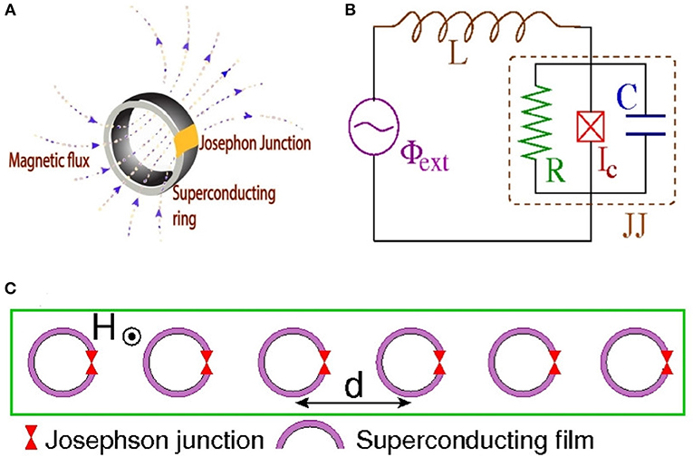
Figure 1. (A) Schematic of a SQUID (superconducting quantum interference device) in a magnetic field. (B) Equivalent electrical circuit. (C) Schematic top view of a one-dimensional periodic array of SQUIDs in a magnetic field H.

SQUID metamaterials are extended systems containing a large number of SQUIDs arranged in various configurations which, from the dynamical systems point of view, can be viewed theoretically as an assembly of weakly coupled non-linear oscillators that inherit the flexibility of their constituting elements (i.e, the SQUIDs). They present a non-linear dynamics laboratory in which numerous classical as well as quantum complex spatio-temporal phenomena can be explored. Recent experiments on SQUID metamaterials have revealed several extraordinary properties, such as negative permeability [26], broad-band tunability [26, 27], self-induced broad-band transparency [28], dynamic multistability and switching [29], as well as coherent oscillations [30]. Moreover, non-linear effects, such as localization of the discrete breather type [31] and non-linear band-opening (non-linear transmission) [32], as well as the emergence of counter-intuitive dynamic states referred to as chimera states in current literature [33–35], have been demonstrated numerically in SQUID metamaterial models [36].

The chimera states, in particular, which were first discovered in rings of non-locally and symmetrically coupled identical phase oscillators [37], have been reviewed thoroughly in recent articles [38–40], are characterized by the coexistence of synchronous and asynchronous clusters of oscillators; their discovery was followed by intense theoretical [41–61] and experimental [62–76] activities, in which chimera states have been observed experimentally or demonstrated numerically in a huge variety of physical and chemical systems.

Here, the possibility for generating chimera states in SQUID metamaterials driven by a time-dependent magnetic flux is demonstrated. These chimera states can be generated from a large variety of initial conditions, and they are characterized using well-established measures. Also, the present work is the first to demonstrate numerically the generation of chimera states while the system is “at rest” (i.e., with zero initial conditions) by using a temporally constant force gradient (i.e, a dc flux gradient) in addition to the time-dependent magnetic flux. In that case, controlled generation of chimera states can be achieved. The SQUIDs in such a metamaterial are coupled together through magnetic dipole-dipole forces due to their mutual inductance. This kind of coupling between SQUIDs falls-off approximately as the inverse cube of their center-to-center distance, and thus it is clearly non-local. However, due to the magnetic nature of the coupling, its strength is weak [27, 30], and thus a nearest-neighbor coupling approach (i.e., a local coupling approach) is often sufficient in capturing the essentials of the dynamics of SQUID metamaterials. Chimera states emerge in SQUID metamaterials with either non-local [33, 35] or local [34] coupling between SQUIDs.

In the next section (Methods), a model for a single SQUID that relies on the equivalent electrical circuit of Figure 1B is described, and the dynamic equation for the flux through the ring of the SQUID is derived and normalized. In the same section, the dynamic equations for a one-dimensional (1D) SQUID metamaterial with non-local coupling are derived, and subsequently they are reduced to the local coupling limit. In section 3 (Results), various types of chimera states are presented and characterized using appropriate measures. In this section, the possibility to generate chimera states with a dc flux gradient, is also explored. A brief discussion is given in section 4 (Discussion).

2. Methods

2.1. The SQUID Oscillator

The simplest version of a SQUID consists of a superconducting ring interrupted by a JJ (Figure 1A), which can be modeled by the equivalent electrical circuit of Figure 1B; according to that model, the SQUID features a self-inductance L, a capacitance C, a resistance R, and a critical current I_c which characterizes an ideal JJ. A “real” JJ (brown-dashed square in Figure 1B) is however modeled as a parallel combination of an ideal JJ, the resistance R, and the capacitance C. When a time-dependent magnetic field is applied to the SQUID in a direction transverse to its ring, the flux threading the SQUID ring induces two types of currents; the supercurrent, which is lossless, and the so-called quasiparticle current which is subject to Ohmic losses. The latter roughly corresponds to the current through the branch containing the resistor R in Figure 1B. The (generally time-dependent) flux threading the ring of the SQUID is described in the model as a flux source, Φ_ext. Many variants of SQUIDs have been studied for several decades (since 1964) and they have found numerous applications in magnetic field sensors, biomagnetism, non-destructive evaluation, and gradiometers, among others [77, 78]. SQUIDs exhibit very rich dynamics including multistability, complex bifurcation structure, and chaotic behavior [79].

The magnetic flux Φ threading the ring of the SQUID is given by

$\begin{array}{ll}\Phi ={\Phi }_{ext}+LI,& (1)\end{array}$

where Φ_ext is the external flux applied to the SQUID, and

$\begin{array}{ll}I=-C\frac{d^2\Phi }{d{t}^2}-\frac{1}{R}\frac{d\Phi }{dt}-I_{c}sin\left(2\pi \frac{\Phi }{{\Phi }_0}\right),& (2)\end{array}$

is the total current induced in the SQUID as provided by the resistively and capacitively shunted junction (RCSJ) model of the JJ [80] (the part of the circuit in Figure 1B contained in the brown-dashed square), Φ₀ is the flux quantum, and t is the temporal variable. The three terms in the right-hand-side of Equation (2) correspond to the current through the capacitor C, the current through the resistor R, and the supercurrent through the ideal JJ, respectively. The combination of Equations (1) and (2) gives

$\begin{array}{ll}C\frac{d^2\Phi }{d{t}^2}+\frac{1}{R}\frac{d\Phi }{dt}+I_{c}sin\left(2\pi \frac{\Phi }{{\Phi }_0}\right)+\frac{\Phi -{\Phi }_{ext}}{L}=0.& (3)\end{array}$

Note that losses decrease with increasing Ohmic resistance R, which is a peculiarity of the SQUID device. The external flux usually consists of a constant (dc) term Φ_dc and a sinusoidal (ac) term of amplitude Φ_ac and frequency ω, i.e., it is of the form

$\begin{array}{ll}{\Phi }_{ext}={\Phi }_{dc}+{\Phi }_{ac}cos(\omega t).& (4)\end{array}$

The normalized form of Equation (3) be obtained by using the relations

$\begin{array}{ll}\varphi =\frac{\Phi }{{\Phi }_0},{\varphi }_{ac,dc}=\frac{{\Phi }_{ac,dc}}{{\Phi }_0},\tau ={\omega }_{LC}t,\Omega =\frac{\omega }{{\omega }_{LC}},& (5)\end{array}$

where ${\omega }_{LC}=1/\sqrt{LC}$ is the inductive-capacitive (L C) SQUID frequency (geometrical frequency), and the definitions

$\begin{array}{ll}\beta =\frac{I_{c}L}{{\Phi }_0}=\frac{{\beta }_L}{2\pi },\gamma =\frac{1}{R}\sqrt{\frac{L}{C}}.& (6)\end{array}$

for the rescaled SQUID parameter and the loss coefficient, respectively. Thus, we get

$\begin{array}{ll}\ddot{\varphi }+\gamma \dot{\varphi }+\varphi +\beta sin(2\pi \varphi )={\varphi }_{dc}+{\varphi }_{ac}cos(\Omega \tau ).& (7)\end{array}$

By substituting γ = 0 and ϕ_ext = 0 and β sin(2πϕ) ≃ β_Lϕ into Equation (7), we get $\ddot{\varphi }+{\Omega }_{SQ}^2\varphi =0$, with ${\Omega }_{SQ}=\sqrt{1+{\beta }_L}$ being the linear eigenfrequency (resonance frequency) of the SQUID. Equation (7) can be also written as

$\begin{array}{ll}\ddot{\varphi }+\gamma \dot{\varphi }=-\frac{d{u}_{SQ}}{d\varphi },& (8)\end{array}$

where

$\begin{array}{ll}{u}_{SQ}=-{\varphi }_{ext}(\tau )\varphi +\frac{1}{2}\left[{\varphi }^2-\frac{\beta }{\pi }cos(2\pi \varphi )\right],& (9)\end{array}$

is the normalized SQUID potential, and

$\begin{array}{ll}{\varphi }_{ext}(\tau )={\varphi }_{dc}+{\varphi }_{ac}cos(\Omega \tau ),& (10)\end{array}$

is the normalized external flux. The SQUID potential u_SQ given by Equation (9) is time-dependent for ϕ_ac ≠ 0 and Ω ≠ 0. Here, parameter values of β_L less than unity (β_L < 1) are considered, in accordance with recent experiments; in that case, u_SQ is a single-well, although non-linear potential. For ϕ_ext = ϕ_dc, there is no time-dependence; however, the shape of u_SQ varies with varying ϕ_dc, as it can be seen in Figure 2. The potential u_SQ is symmetric around a particular ϕ for integer and half-integer values of ϕ_dc. In Figures 2A,C,E, the potential u_SQ is symmetric around ϕ = 0, 0.5, and 1, respectively. For all the other values of ϕ_dc, the potential u_SQ is asymmetric; this asymmetry of u_SQ allows for chaotic behavior to appear in an ac and dc driven single SQUID through period-doubling bifurcation cascades. Such cascades and the subsequent transition to chaos are prevented by a symmetric u_SQ which renders the SQUID a symmetric system in which period-doubling bifurcations are suppressed [81]. Actually, suppression of period-doubling bifurcation cascades due to symmetry occurs in a large class of systems, including the sinusoidally driven-damped pendulum.

FIGURE 2

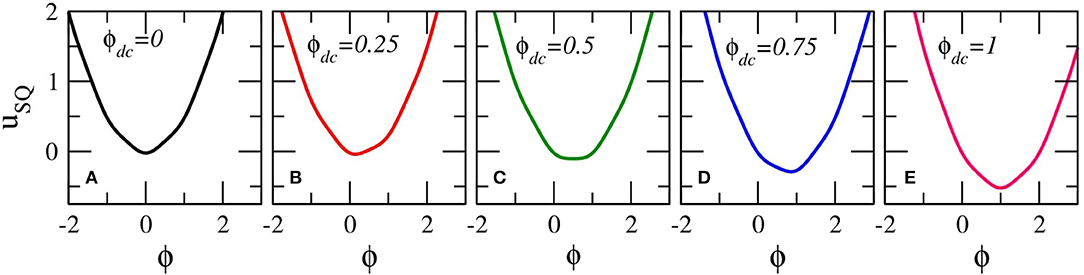
Figure 2. SQUID potential curves u_SQ(ϕ) for β_L = 0.86, ϕ_ac = 0, and (A) ϕ_dc = 0; (B) ϕ_dc = 0.25; (C) ϕ_dc = 0.5; (D) ϕ_dc = 0.75; (E) ϕ_dc = 1.0.

For zero dc flux, the strength of the SQUID non-linearity increases with increasing ac flux amplitude ϕ_ac. This effect is illustrated in Figure 3 in which the flux amplitude—driving frequency (ϕ_max − Ω) curves, i.e., the resonance curves, for four values of ϕ_ac spanning four orders of magnitude are shown (for ϕ_dc = 0). In Figure 3A, for ϕ_ac = 0.0001, the SQUID is in the linear regime and thus its ϕ_max − Ω curve is apparently symmetric around the linear SQUID eigenfrequency, ${\Omega }_{SQ}=\sqrt{1+{\beta }_L}\simeq 1.364$. Weak non-linear effects begin to appear in Figure 3B, for ϕ_ac = 0.002, in which the curve is slightly bended to the left. In Figure 3C, for ϕ_ac = 0.01, the non-linear effects are already strong enough to generate a multistable ϕ_max − Ω curve. In Figure 3D, for ϕ_ac = 0.1, the SQUID is in the strongly non-linear regime and the ϕ_max − Ω curve has acquired a snake-like form. Indeed, the curve “snakes” back and forth within a narrow frequency region via successive saddle-node bifurcations [79]. Note that in Figures 3C,D, the frequency region with the highest multistability is located around the geometrical frequency of the SQUID, i.e., at Ω ≃ 1 (the L C frequency in normalized units). Inasmuch the frequency at which ϕ_max is highest can be identified with the “resonance” frequency of the SQUID, it can be observed that this resonance frequency lowers with increasing ϕ_ac from the linear SQUID eigenfrequency Ω_SQ to the inductive-capacitive (geometrical) frequency Ω ≃ 1. Thus, the resonance frequency of the SQUID, where its multistability is highest, can be actually tuned by non-linearity, i.e., by varying the ac flux amplitude ϕ_ac. Note that the multistability of the SQUID is a purely dynamic effect, which is not related to any local minima of the SQUID potential (which is actually single-welled for the values of β_L considered here, i.e., for β_L < 1).

FIGURE 3

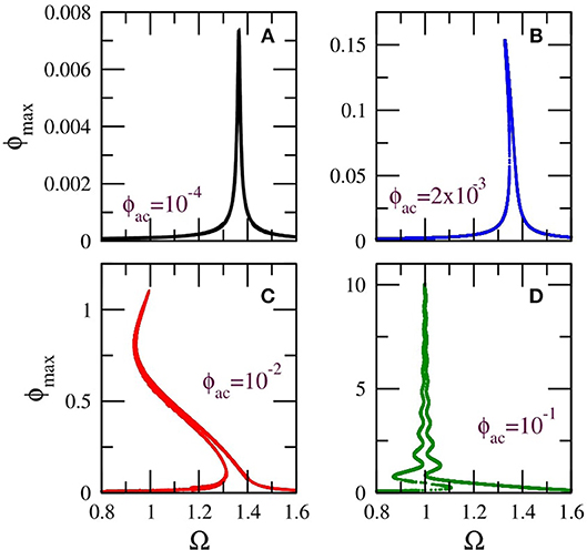
Figure 3. Flux amplitude–driving frequency (ϕ_max − Ω) curves for a SQUID with β_L = 0.86, γ = 0.01, ϕ_dc = 0, and (A) ${\varphi }_{ac}=10^{-4}$, (B) ${\varphi }_{ac}=2\times 10^{-3}$, (C) ${\varphi }_{ac}=10^{-2}$, (D) ${\varphi }_{ac}=10^{-1}$.

For ϕ_dc ≠ 0, chaotic behavior appears in wide frequency intervals below the geometrical frequency (Ω = 1) for relatively high ϕ_ac. As it was mentioned above, the SQUID potential u_SQ is asymmetric for ϕ_dc ≠ 0, and thus the SQUID can make transitions to chaos through period-doubling cascades [79]. In the bifurcation diagram shown in Figure 4A, the flux ϕ is plotted at the end of each driving period T = 2π/Ω for several tenths of driving periods (transients have been rejected) as a function of the driving frequency Ω. This bifurcation diagram reveals multistability as well as a reverse period-doubling cascade leading to chaos. That reverse cascade, specifically, begins at Ω = 0.64 with a stable period-2 solution (i.e., whose period is two times that of the driving period T). A period-doubling occurs at Ω = 0.638 resulting in a stable period-4 solution. The next period-doubling, at Ω = 0.62, results in a stable period-8 solution. The last period-doubling bifurcation which is visible in this scale occurs at Ω = 0.614 and results in a stable period-16 solution. More and more period-doubling bifurcations very close to each other lead eventually to chaos at Ω = 0.6132. Note that another stable multiperiodic solution is present in the frequency interval shown in Figure 4A. A typical chaotic attractor of the SQUID is shown on the $\varphi -\dot{\varphi }$ phase plane in Figure 4B for Ω = 0.6.

FIGURE 4

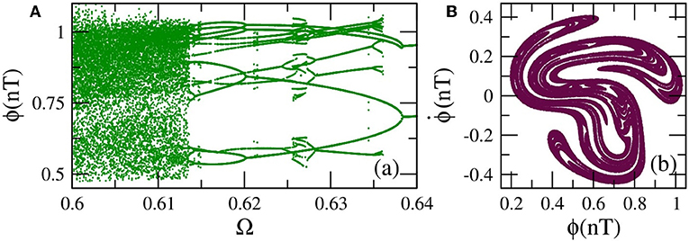
Figure 4. (A) Bifurcation diagram of ϕ(nT) as a function of the driving frequency Ω, for β_L = 0.86, γ = 0.01, ϕ_dc = 0.36, and ϕ_ac = 0.18. (B) A typical chaotic attractor on the $\varphi -\dot{\varphi }$ phase-plane for Ω = 0.6. The other parameters are as in (A).

2.2. SQUID Metamaterials: Modeling

2.2.1. Flux Dynamics Equations

Consider a one-dimensional periodic arrangement of N identical SQUIDs in a transverse magnetic field H as in Figure 1C, whose center-to-center distance is d and they are coupled through (non-local) magnetic dipole-dipole forces [33]. The magnetic flux Φ_n threading the ring of the n−th SQUID is

$\begin{array}{ll}{\Phi }_n={\Phi }_{ext}+L{I}_n+L{\displaystyle \sum _{m\ne n}}{\lambda }_{|m-n|}{I}_m,& (11)\end{array}$

where n, m = 1, …, N, Φ_ext is the external flux in each SQUID, λ_|m−n| = M_|m−n|/L is the dimensionless coupling coefficient between the SQUIDs at the sites m and n, with M_|m−n| being their mutual inductance, and

$\begin{array}{ll}-I_n=C\frac{d^2{\Phi }_n}{d{t}^2}+\frac{1}{R}\frac{d{\Phi }_n}{dt}+I_{c}sin\left(2\pi \frac{{\Phi }_n}{{\Phi }_0}\right)& (12)\end{array}$

is the current in the n−th SQUID as given by the RCSJ model [80]. The combination of Equations (11) and (12) gives

$\begin{array}{c}C\frac{d^2{\Phi }_n}{d{t}^2}+\frac{1}{R}\frac{d{\Phi }_n}{dt}+I_{c}sin\left(2\pi \frac{{\Phi }_n}{{\Phi }_0}\right)\\ +\frac{1}{L}{\displaystyle \sum _{m=1}^N}{\left({\widehat{\Lambda }}^{-1}\right)}_{nm}({\Phi }_m-{\Phi }_{ext})=0,& (13)\end{array}$

where ${\widehat{\Lambda }}^{-1}$ is the inverse of the symmetric N × N coupling matrix with elements

$\begin{array}{ll}{\widehat{\Lambda }}_{nm}=\{\begin{array}{ll}1,\hfill & \text{if }m=n;\hfill \\ {\lambda }_{|m-n|}={\lambda }_1|m-n{|}^{-3},\hfill & \text{if }m\ne n,\hfill \end{array}& (14)\end{array}$

with λ₁ being the coupling coefficient between nearest neighboring SQUIDs. Note that due to the geometry of the SQUID metamaterial considered here, which is planar, and according to standard conventions for loops carrying current flowing in the same direction, the mutual inductance M_|m−n| between the n−th and the m−th SQUIDs is negative (M_|m−n| < 0 for any n, m with n ≠ m). Thus, since L > 0, the coupling strength λ_|m−n| is negative. The dependence of the coupling strength on the center-to-center distance between SQUIDs in Equation (14) is due to their mutual inductance M_|m−n|, which can be obtained using basic expressions from electromagnetism. The magnetic field generated by a wire loop, at a distance d greater than its dimensions, is given by the Biot-Savart law as $B=\frac{{\mu }_0}{4\pi }\frac{\pi r_w^2{I}_w}{d^3}$, where I_w is the current in the wire, r_w is the radius of the loop, which approximate the SQUID geometry, d is the distance from the center of the loop, and μ₀ is the permeability of the vacuum. The magnitude of the mutual inductance between two such (identical) loops lying on the same plane is given by

$\begin{array}{ll}M=\frac{B\pi r_w^2}{I_w}=\frac{{\mu }_0}{4\pi }\frac{{(\pi r_w^2)}^2}{d^3}\propto d^{-3},& (15)\end{array}$

where it is assumed that the field B is constant over the area of each loop, $\pi r_w^2$. For square loops of side a, the radius r_w should be replaced by $a/\sqrt{\pi }$. Equation (15) explains qualitatively the inverse cube distance-dependence of the coupling strength λ_|m−n| between SQUIDs.

In normalized form Equation (13) reads (n = 1, …, N)

$\begin{array}{ll}{\ddot{\varphi }}_n+\gamma {\dot{\varphi }}_n+\beta sin(2\pi {\varphi }_n)={\displaystyle \sum _{m=1}^N}{\left({\widehat{\Lambda }}^{-1}\right)}_{nm}({\varphi }_{ext}-{\varphi }_m),& (16)\end{array}$

where Equation (5) and the definitions Equation (6) have been used. When nearest-neighbor coupling is only taken into account, Equation (16) reduces to the simpler form

$\begin{array}{l}{\ddot{\varphi }}_n+\gamma {\dot{\varphi }}_n+{\varphi }_n+\beta sin(2\pi {\varphi }_n)=\lambda ({\varphi }_{n-1}+{\varphi }_{n+1})\\ +(1-2\lambda ){\varphi }_{ext},& (17)\end{array}$

where λ = λ₁.

2.2.2. Local and Non-local Linear Frequency Dispersion

Equation (11) with Φ_ext = 0 can be written in matrix form as

$\begin{array}{ll}L\widehat{\Lambda }\overrightarrow{I}=\overrightarrow{\Phi },& (18)\end{array}$

where the elements of the coupling matrix $\widehat{\Lambda }$ are given in Equation (14), and $\overrightarrow{I}$, $\overrightarrow{\Phi }$ are N−dimensional vectors with components I_n, Φ_n, respectively. The linearized equation for the current in the n−th SQUID, in the lossless case (R → ∞), is given from Equation (12) as

$\begin{array}{ll}-\overrightarrow{I}=C\frac{d^2}{d{t}^2}\overrightarrow{\Phi }+2\pi \frac{I_c}{{\Phi }_0}\overrightarrow{\Phi },& (19)\end{array}$

where the approximation sin(x) ≃ x has been employed. By substituting Equation (19) into Equation (18), we get

$\begin{array}{ll}\widehat{\Lambda }\left(\frac{1}{{\omega }_{LC}^2}\frac{d^2}{d{t}^2}\overrightarrow{\Phi }+{\beta }_L\overrightarrow{\Phi }\right)+\overrightarrow{\Phi }=0.& (20)\end{array}$

In component form, the corresponding equation reads

$\begin{array}{ll}{\displaystyle \sum _m}{\widehat{\Lambda }}_{nm}\left(\frac{1}{{\omega }_{LC}^2}\frac{d^2}{d{t}^2}{\Phi }_m+{\beta }_L{\Phi }_m\right)+{\Phi }_n=0,& (21)\end{array}$

or, in normalized form

$\begin{array}{ll}{\displaystyle \sum _m}{\widehat{\Lambda }}_{nm}\left(\frac{1}{{\omega }_{LC}^2}{\ddot{\varphi }}_m+{\beta }_L{\varphi }_m\right)+{\varphi }_n=0,& (22)\end{array}$

where the overdots denote derivation with respect to the normalized time τ = ω_LCt.

Substitute the trial (plane wave) solution

$\begin{array}{ll}{\varphi }_n={exp}^{i(\kappa n-\Omega \tau )},& (23)\end{array}$

where κ is the dimensionless wavenumber (in units of d⁻¹), into Equation (22) to obtain

$\begin{array}{ll}{\Omega }^2=\frac{1}{S}(1+{\beta }_{L}S),& (24)\end{array}$

where

$\begin{array}{ll}S={\displaystyle \sum _m}{\widehat{\Lambda }}_{nm}{exp}^{i\kappa (m-n)}.& (25)\end{array}$

It can be shown that, for the infinite system, the function S is

$\begin{array}{ll}S=1+2\lambda {\displaystyle \sum _{s=1}^{\infty }}\frac{cos(\kappa s)}{|s{|}^3}=1+2\lambda C{i}_3(\kappa ),& (26)\end{array}$

where s = m − n, and Ci₃(κ) is a Clausen function. Putting Equation (26) into Equation (24), we obtain the non-local frequency dispersion for the 1D SQUID metamaterial as

$\begin{array}{ll}{\Omega }_{\kappa }=\sqrt{\frac{{\Omega }_{SQ}^2+2\lambda {\beta }_{L}C{i}_3(\kappa )}{1+2\lambda C{i}_3(\kappa )}},& (27)\end{array}$

where ${\Omega }_{SQ}^2=1+{\beta }_L$. In the case of local (nearest-neighbor) coupling the Clausen function Ci₃(κ) is replaced by cos(κ). Then, by neglecting terms of order λ² or higher, the local frequency dispersion

$\begin{array}{ll}{\Omega }_{\kappa }\simeq \sqrt{{\Omega }_{SQ}^2-2\lambda cos(\kappa )}& (28)\end{array}$

is obtained.

The linear frequency dispersion Ω = Ω_κ, calculated for non-local and local coupling from Equations (27) and (28), respectively, is plotted in Figure 5 for three values of the coupling coefficient λ. The differences between the non-local and local dispersion are rather small, especially for low values of λ, i.e., for λ = −0.02 (Figure 5A), which are mostly considered here. Although the linear frequency bands are narrow, the bandwidth ΔΩ = Ω_max − Ω_min increases with increasing λ. For simplicity, the bandwidth ΔΩ can be estimated from Equation (28); from that equation the minimum and maximum frequencies of the band can be approximated by ${\Omega }_{min,max}\simeq {\Omega }_{SQ}\left(1\pm \frac{\lambda }{{\Omega }_{SQ}^2}\right)$, so that

$\begin{array}{ll}\Delta \Omega \simeq \frac{2|\lambda |}{{\Omega }_{SQ}}.& (29)\end{array}$

That is, the bandwidth is roughly proportional to the magnitude of λ. Note that for physically relevant parameters, the minimum frequency of the linear band is well above the geometrical (i.e., inductive-capacitive) frequency of the SQUIDs in the metamaterial. Thus, for strong non-linearity, for which the resonance frequency of the SQUIDs is close to the geometrical one (Ω = 1), no plane waves can be excited. It is this frequency region where localized and other spatially inhomogeneous states, such as chimera states are expected to emerge (given also the extreme multistability of individual SQUIDs there).

FIGURE 5

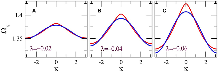
Figure 5. Linear frequency dispersion Ω = Ω_κ for non-local (red) and local (blue) coupling, for β_L = 0.86, and (A) λ = −0.02, (B) λ = −0.04; (C) λ = −0.06.

3. Results

3.1. Chimeras and Other Spatially Inhomogeneous States

Equation (16) are integrated numerically in time with free-end boundary conditions (ϕ_N+1 = ϕ₀ = 0) using a fourth-order Runge-Kutta algorithm with time-step h = 0.02. The initial conditions have been chosen so that they lead to chimera states. It should be noted that chimera states can be obtained from a huge variety of initial conditions. Here we choose

$\begin{array}{ll}{\varphi }_n(\tau =0)=\{\begin{array}{ll}1,\hfill & \text{for }{n}_{\ell }<n\le n_r;\hfill \\ 0,\hfill & \text{otherwise},\hfill \end{array}& (30)\end{array}$

$\begin{array}{llll}{\dot{\varphi }}_n(\tau =0)& =& 0,& (31)\end{array}$

with n_ℓ = 18 and n_r = 36. The number of SQUIDs in the metamaterial in all calculations below is N = 54. Equation (16) are first integrated in time for a relatively long time-interval, 10⁷T time-units, where T = 2π/Ω is the driving period, so that the system has reached a steady-state. While the SQUID metamaterial is in the steady-state, Equation (16) are integrated for τ_sst = 1000 T more time-units. Then, the profiles of the time-derivatives of the fluxes, averaged over the driving period T, i.e.,

$\begin{array}{ll}{\langle {\dot{\varphi }}_n\rangle }_T=\frac{1}{T}{\displaystyle {\int }_0^T}{\dot{\varphi }}_{n}d\tau ,n=1,\dots ,N,& (32)\end{array}$

are mapped as a function of τ. Such maps are shown in Figure 6, for several values of the ac flux amplitude, ϕ_ac. In these maps, areas with uniform colorization indicate that the SQUID oscillators there are synchronized, while areas with non-uniform colorization indicate that they are desynchronized.

FIGURE 6

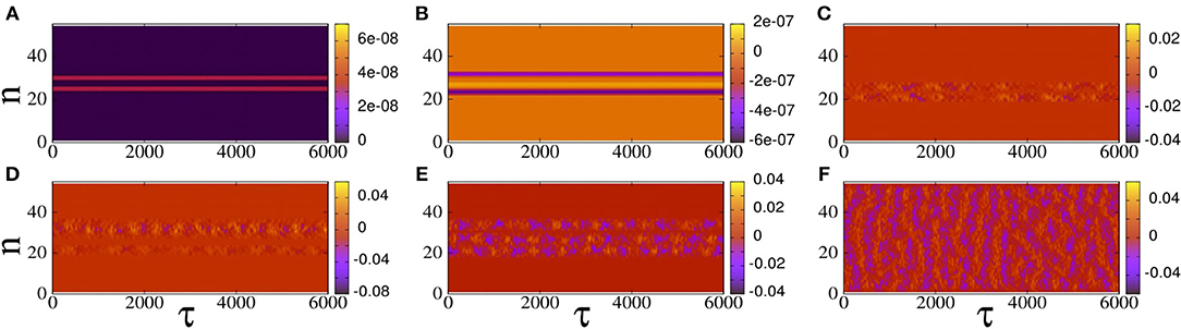
Figure 6. Maps of $\langle {\dot{\varphi }}_n\rangle (\tau )$ on the n − τ plane for β_L = 0.86, γ = 0.01, λ = −0.02, Ω = 1.01, N = 54, ϕ_dc = 0, and (A) ϕ_ac = 0.02, (B) ϕ_ac = 0.04, (C) ϕ_ac = 0.06, (D) ϕ_ac = 0.08, (E) ϕ_ac = 0.10, (F) ϕ_ac = 0.12.

In Figures 6A,B, i.e., for low values of ϕ_ac, chimera states are not excited since the ${\langle {\dot{\varphi }}_n\rangle }_T$ are practically zero during the steady-state integration time. However, this does not mean that the state of the SQUID metamaterial is spatially homogeneous, as we shall see below. For higher values of ϕ_ac, chimera states begin to appear, in which one or more desynchronized clusters of SQUID oscillators roughly in the middle of the SQUID metamaterial are visible (Figures 6C–E). For even higher values of ϕ_ac, as can be seen in Figure 6F, the whole SQUID metamaterial is desynchronized. In order to quantify the degree of synchronization for SQUID metamaterials at a particular time-instant τ, the magnitude of the complex synchronization (Kuramoto) parameter r is calculated, where

$\begin{array}{ll}r(\tau )=\left|\Psi (\tau )\right|=\frac{1}{N}\left|{\displaystyle \sum _n{e}^{i[2\pi {\varphi }_n(\tau )]}}\right|.& (33)\end{array}$

Note that the phase in the earlier equation, which is enclosed in the square brackets, 2πϕ_n(τ), or 2πΦ_n(τ)/Φ₀ in natural units, is actually the argument of the sine term in Equation (13). Below, two averages of r(τ) are used for the characterization of a particular state of SQUID metamaterials, i.e., the average of r(τ) over the driving period T, 〈r〉_T(τ), and the average of r(τ) over the steady-state integration time 〈r〉_sst. These are defined, respectively, as

$\begin{array}{ll}\langle r{(\tau )}_T\rangle =\frac{1}{T}{\displaystyle {\int }_0^{T}r}(\tau )d\tau ,{\langle r\rangle }_{sst}=\frac{1}{{\tau }_{sst}}{\displaystyle {\int }_0^{{\tau }_{sst}}r}(\tau )d\tau .& (34)\end{array}$

The calculated 〈r〉_T(τ) for the states shown in Figure 6, clarify further their nature. In Figure 7A, 〈r〉_T(τ) is plotted as a function of time τ for all the six states presented in Figure 6. It can be seen that for ϕ_ac = 0.02 and 0.04 (black and red curves), calculated for the states of the SQUID metamaterial in Figures 6A,B, respectively, 〈r〉_T(τ) is constant in time, although less than unity. For such states, 〈r〉_T(τ) = 〈r〉_sst, where 〈r〉_sst can be inferred from Figure 7B for the curves of interest to be 〈r〉_sst ≃ 0.972 and 〈r〉_sst ≃ 0.894 for ϕ_ac = 0.02 and 0.04, respectively. The lack of fluctuations indicates that these states consist of “clusters” in which the SQUID oscillators are synchronized together. However, the clusters are not synchronized to each other, resulting in a partially synchronized state with 〈r〉_T(τ) < 1. The exact nature of these partially synchronized states can be clarified by plotting the flux profiles ϕ_n at the end of the steady-state integration time as shown in Figures 7C,D. In these figures, it can be observed that all but a few SQUID oscillators are synchronized; in addition, those few SQUIDs execute high-amplitude flux oscillations. Moreover, it has been verified that the frequency of all the flux oscillations is that of the driving, Ω. Such states can be classified as discrete breathers/multi-breathers, i.e., spatially localized and time-periodic excitations which have been proved to emerge generically in non-linear networks of weakly coupled oscillators [82]. In the present case, the multibreathers shown in Figures 7C,D can be further characterized as dissipative ones [83], since they emerge through a delicate balance of input power and intrinsic losses. They have been investigated in some detail in SQUID metamaterials in one and two dimensions [31, 84–86], as well as in SQUID metamaterials on two-dimensional Lieb lattices [87].

FIGURE 7

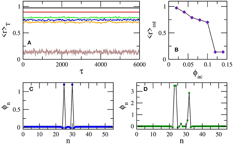
Figure 7. (A) The magnitude of the synchronization parameter averaged over the driving period, 〈r〉_T, as a function of time τ for β_L = 0.86, γ = 0.01, λ = −0.02, Ω = 1.01, N = 54, ϕ_dc = 0, and ϕ_ac = 0.02 (black), ϕ_ac = 0.04 (red), ϕ_ac = 0.06 (green), ϕ_ac = 0.08 (blue), ϕ_ac = 0.10 (orange), ϕ_ac = 0.12 (brown). (B) The magnitude of the synchronization parameter averaged over the steady-state integration time τ_sst, 〈r〉_sst, as a function of the ac flux amplitude ϕ_ac. The other parameters are as in (A). (C) The flux profile ϕ_n for ϕ_ac = 0.02 and the other parameters as in (A). (D) The flux profile ϕ_n for ϕ_ac = 0.04 and the other parameters as in (A).

The corresponding 〈r〉_T(τ) for the states shown in Figures 6C–F, are shown in Figure 7A as green, blue, orange, and brown curves, respectively. In these curves there are apparently fluctuations around their temporal average over the steady-state integration time (shown in Figure 7B). These fluctuations are typically associated with the level of metastability of the chimera states [88, 89]; an appropriate measure of metastability for SQUID metamaterials is the full-width half-maximum (FWHM) of the distribution of 〈r〉_T [33]. The FWHM can be used to compare the metastability levels of different chimera states. For synchronized (spatially homogeneous) and partially synchronized states, such as those in Figures 6A,B, the FWHM of the corresponding distribution of the values of 〈r〉_T is practically zero.

Another set of initial conditions which gives rise to chimera states is of the form [34]

$\begin{array}{ll}{\varphi }_n(\tau =0)=\frac{1}{2}cos\left(\frac{2j\pi n}{N}\right),{\dot{\varphi }}_n(\tau =0)=0,n=1,\dots ,N.& (35)\end{array}$

The initial conditions in Equation (35) allow for generating multiclustered chimera states, in which the number of clusters depends on j. In Figures 8A,B, maps of ${\langle {\dot{\varphi }}_n\rangle }_T$ on the n − τ plane for j = 1 and j = 2, respectively, are shown. In Figure 8A, three large clusters can be distinguished; in the two of them, the SQUID oscillators are synchronized, while in the third one, in between the two sychronized clusters, the SQUID oscillators are desynchronized. The flux profile ϕ_n of that state at the end of the steady-state integration time τ_sst = 6, 000, is shown in Figure 8C as blue circles (the black curve is a guide to the eye) along with the initial condition (red curve). It can be seen that two more desynchronized clusters at the ends of the metamaterial, which are rather small (they consist of only a few SQUIDs each), are visible. Obviously, the synchronized clusters correspond to the spatial interval indicated by the almost horizontal segments in the ϕ_n profile. The corresponding ${\langle {\dot{\varphi }}_n\rangle }_T$ map and flux profile ϕ_n for j = 2 is shown in Figures 8B,D, respectively. In this case, a number of six (6) synchronized clusters and seven (7) desynchronized clusters are visible in both Figures 8B,D. In Figure 8D, the red curve is the initial condition from Equation (35) with j = 2. Chimera states with even more “heads” can be generated from the initial condition Equation (35) for j > 2 in larger systems (here N = 54).

FIGURE 8

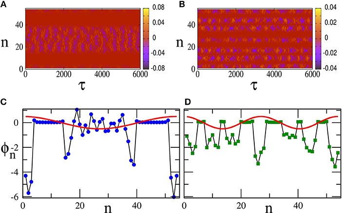
Figure 8. (A) Map of ${\langle {\dot{\varphi }}_n\rangle }_T$ on the n − τ plane for β_L = 0.86, γ = 0.01, λ = −0.02, Ω = 1.01, N = 54, ϕ_dc = 0, ϕ_ac = 0.1, and initial conditions given by Equation (35) with j = 1. (B) Same as in (A) with initial conditions given by Equation (35) with j = 2. (C) Flux profile ϕ_n at the end of the steady-state integration time (blue circles, the black line is a guided to the eye), obtained with the initial conditions Equation (35) with j = 1 (red curve). (D) Flux profile ϕ_n at the end of the steady-state integration time (blue circles, the black line is a guided to the eye), obtained with the initial conditions Equation (35) with j = 2 (red curve).

Similar chimera states can be generated with local (nearest-neighbor) coupling between the SQUIDs of the metamaterial. For that purpose, Equation (17) is integrated in time using a fourth order Runge-Kutta algorithm with free-end boundary conditions and the initial conditions of Equation (30). As above, in order to eliminate transients and reach a steady-state, Equation (17) is integrated for 10⁷ T time units and the results are discarded. Then, Equation (17) is integrated for ${\tau }_{sst}=10^{3}T$ more time units (steady-state integration time), and ${\langle {\dot{\varphi }}_n\rangle }_T$ is mapped on the n − τ plane (Figure 9). The emerged states are very similar to those shown in Figure 6, which is the case of non-local coupling between the SQUIDs. In particular, the states shown in Figures 9A–C, have been generated for exactly the same parameters and initial-boundary conditions as those in Figures 6C,E,F, respectively, i.e, for ϕ_ac = 0.06, 0.1, and 0.12. Note that the state of the SQUID metamaterial for ϕ_ac = 0.12 is completely desynchronized both in Figures 6F, 9C. One may also compare the plots of the corresponding 〈r〉_T as a function of τ, which are shown in Figure 9D for the local coupling case. The averages of r over the steady-state integration time τ_sst for ϕ_ac = 0.06, 0.1, 0.12 are respectively, 〈r〉_sst = 0.757, 0.656, 0.136 for the non-local coupling case and 〈r〉_sst = 0.743, 0.656, 0.146 for the local coupling case. The probability distribution function of the values of 〈r〉_T, pdf(〈r〉_T), for the three states in Figures 9A–C are shown in Figures 9E–G, respectively. As it was mentioned above, the FWHM of such a distribution is a measure of the metastability of the corresponding chimera state. The FWHM for the distributions in Figures 9E,F, calculated for the chimera states shown in Figures 9A,B, are respectively 0.003 and 0.0215. Thus, it can be concluded that the chimera state of Figure 9B is more metastable than that in Figure 9A. The distribution in Figure 9G has a FWHM much larger than the ones of the distributions in Figures 9E,F as expected, since it has been calculated for the completely desynchronized state of Figure 9C. Note that 10⁶ values of 〈r〉_T have been used to obtain each of the three distributions. Also, these distributions are normalized such that their area sums to unity.

FIGURE 9

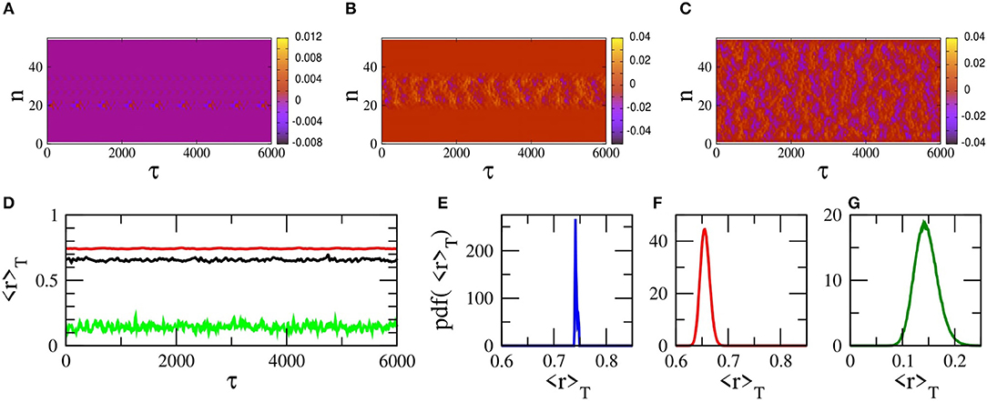
Figure 9. (A) Map of ${\langle {\dot{\varphi }}_n\rangle }_T$ on the n − τ plane for β_L = 0.86, γ = 0.01, λ = −0.02, Ω = 1.01, N = 54, ϕ_dc = 0, ϕ_ac = 0.06, and initial conditions given by Equation (30). (B) Same as in (A) but with ϕ_ac = 0.10. (C) Same as in (A,B) but with ϕ_ac = 0.12. (D) The magnitude of the synchronization parameter averaged over the driving period, 〈r〉_T, as a function of time τ for ϕ_ac = 0.06 (red), ϕ_ac = 0.1 (black), and ϕ_ac = 0.12 (green). The other parameters are as in (A). (E) The distribution of 10⁶ values of 〈r〉_T, pdf(〈r〉_T), for the chimera state shown in (A). (F) Same as in (E) for the chimera state shown in (B). (G) Same as in (E,F) for the completely desynchronized state shown in (C).

The chimera states do not result from destabilization of the synchronized state of the SQUID metamaterial; instead, they coexist with the latter, which can be reached simply by integrating the relevant flux dynamics equations with zero initial conditions, i.e., with ϕ_n(τ = 0) = 0 and ${\dot{\varphi }}_n(\tau =0)=0$ for any n. In order to reach a chimera state, on the other hand, appropriately chosen initial conditions, such as those in Equations (30) or (35) have to be used. However, one cannot expect that the synchronized state is stable over the whole external parameter space, i.e., the ac flux amplitude ϕ_ac, the frequency of the ac flux field Ω, and the dc flux bias ϕ_dc. In order to explore the stability of the synchronized state of the SQUID metamaterial, the magnitude of the synchronization parameter averaged over the steady-state integration time, 〈r〉_sst, is calculated and then mapped on the ϕ_dc − ϕ_ac parameter plane. For each pair of ϕ_ac and ϕ_dc values, the SQUID metamaterial is initialized with zeros (it is at “rest”). Once again, the frequency Ω is chosen to be very close to the geometrical resonance Ω_LC (Ω ≃ 1). In Figure 10, maps of 〈r〉_sst on the ϕ_dc − ϕ_ac plane are shown for four driving frequencies Ω around unity. These maps are a kind of “synchronization phase diagrams”, in which 〈r〉_sst = 1 indicates a synchronized state while 〈r〉_sst < 1 indicates a partially or completely desynchronized state. In all subfigures, but perhaps most clearly seen in Figure 10C (for Ω = 1.01) there are abrupt transitions between completely synchronized (red areas) and completely desynchronized (light blue areas) states. It can be verified by inspection of the flux profiles (not shown) that these synchronization-desynchronization transitions do not go through a stage in which chimera states are generated; instead, the destabilization of a synchronized state results either in a completely desynchronized state (light blue areas) or a clustered state (green areas). Thus, it seems that chimera states cannot be generated when the SQUID metamaterial is initially at “rest,” i.e., with zero initial conditions. As we shall see in the next subsection, this is not true for a position-dependent external flux ϕ_ext = ϕ_ext (n).

FIGURE 10

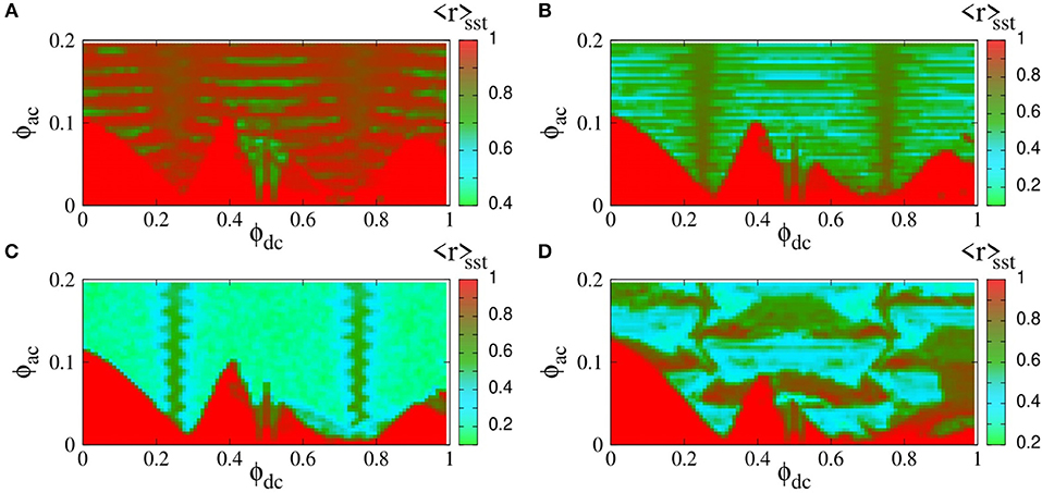
Figure 10. Map of the magnitude of the synchronization parameter averaged over the steady-state integration time, 〈r〉_sst, on the dc flux bias–ac flux amplitude (ϕ_dc − ϕ_ac) parameter plane, for β_L = 0.86, γ = 0.01, λ = −0.02, N = 54, and (A) Ω = 1.03, (B) Ω = 1.02, (C) Ω = 1.01, (D) Ω = 0.982.

3.2. Chimera Generation by dc Flux Gradients

3.2.1. Modified Flux Dynamics Equations

In obtaining the results of Figure 10, a spatially homogeneous dc flux ϕ_dc over the whole SQUID metamaterial is considered. Although, all the chimera states presented here are generated at ϕ_dc = 0, such states can be also generated in the presence of a spatially constant, non-zero ϕ_dc, by using appropriate initial conditions (not shown here). In this subsection, the generation of chimera states in SQUID metamaterials driven by an ac flux and biased by a dc flux gradient is demonstrated, for the SQUID metamaterial being initially at “rest.” The application of a dc flux gradient along the SQUID metamaterial is experimentally feasible with the set-up of Zhang et al. [28]. Consider the SQUID metamaterial model in section 2.2.1 in the case of local coupling (for simplicity), in which the dc flux is assumed to be position-dependent, i.e., ${\varphi }_{dc}={\varphi }_n^{dc}$. Then, Equation (17) can be easily modified to become

$\begin{array}{ll}{\ddot{\varphi }}_n+\gamma {\dot{\varphi }}_n+{\varphi }_n+\beta sin(2\pi {\varphi }_n)={\varphi }_n^{eff}(\tau )+\lambda ({\varphi }_{n-1}+{\varphi }_{n+1}),& (36)\end{array}$

where

$\begin{array}{ll}{\varphi }_n^{eff}={\varphi }_n^{ext}-\lambda ({\varphi }_{n-1}^{ext}+{\varphi }_{n+1}^{ext}),& (37)\end{array}$

with

$\begin{array}{ll}{\varphi }_n^{ext}={\varphi }_n^{dc}+{\varphi }_{ac}cos(\Omega \tau ).& (38)\end{array}$

In the following, the dc flux function ${\varphi }_n^{dc}$ is assumed to be of the form

$\begin{array}{ll}{\varphi }_n^{dc}=\frac{n-1}{N-1}{\varphi }_{max}^{dc},n=1,\dots ,N,& (39)\end{array}$

so that the dc flux bias increases linearly from zero (for the SQUID at n = 1) to ${\varphi }_{max}^{dc}$ (for the SQUID at the n = N).

3.2.2. Controlled Generation of Chimera States

Equations (36) are integrated numerically in time with free-end boundary conditions (Equation 36) using a fourth-order Runge-Kutta algorithm with time-step h = 0.02. The SQUID metamaterial is initially at “rest,” i.e.,

$\begin{array}{ll}{\varphi }_n(\tau =0)=0,{\dot{\varphi }}_n(\tau =0)=0,n=1,\dots ,N.& (40)\end{array}$

This system is integrated for 10⁵T time units to eliminate the transients and then for more ${\tau }_{sst}=10^{5}T$ time units during which the temporal averages 〈r〉_sst and 〈r〉_T(τ) are calculated. Note that the transients die-out faster in this case since the SQUID metamaterial is initialized with zeros. Typical flux profiles ϕ_n, plotted at the end of the steady-state integration time are shown in Figures 11A–I. The varying parameter in this case is ${\varphi }_{max}^{dc}$, which actually determines the gradient of the dc flux. The state of the SQUID metamaterial remains almost homogeneous in space for ${\varphi }_{max}^{dc}$ increasing from zero to ${\varphi }_{max}^{dc}=0.22$. At that critical value of ${\varphi }_{max}^{dc}$, the spatially homogeneous (almost synchronized) state breaks down, for several SQUIDs close to n = N become desynchronized with the rest (because the dc flux is higher at this end). The number of desynchronized SQUIDs for ${\varphi }_{max}^{dc}=0.25$ is about 6−7 (Figure 11A). For further increasing ${\varphi }_{max}^{dc}$, more and more SQUIDs become desynchronized, until they form a well-defined desynchronized cluster (Figure 11B for ${\varphi }_{max}^{dc}=0.30$). As ${\varphi }_{max}^{dc}$ continues to increase, the desynchronized cluster clearly shifts to the left, i.e., toward n = 1 (Figures 11C–E). Further increase of ${\varphi }_{max}^{dc}$ generates a second desynchronized cluster around n = N for ${\varphi }_{max}^{dc}=0.50$ (Figure 11F), which persists for values of ${\varphi }_{max}^{dc}$ at least up to 0.65. With the formation of the second desynchronized cluster, the first one clearly becomes smaller and smaller with increasing ${\varphi }_{max}^{dc}$ (see Figures 11F–I). Above, the expression “almost homogeneous” was used instead of simply “homogeneous,” because complete homogeneity is not possible due to the dc flux gradient. However, for ${\varphi }_{max}^{dc}<0.22$, the degree of homogeneity (synchronization) is more than 99%, i.e., the values of the synchronization parameter 〈r〉_sst are higher than 0.99 (〈r〉_sst > 0.99). The dependence of 〈r〉_sst on ${\varphi }_{max}^{dc}$ for several values of the ac flux amplitude ϕ_ac is shown in Figure 11J. The SQUID metamaterial remains in an almost synchronized state (with 〈r〉_sst > 0.96 below a critical value of ${\varphi }_{max}^{dc}$, which depends on the ac flux amplitude ϕ_ac. That critical value of ${\varphi }_{max}^{dc}$ is lower for higher ϕ_ac. For values of ${\varphi }_{max}^{dc}$ higher than the critical one, 〈r〉_sst gradually decreases until it saturates at 〈r〉_sst ≃ 0.12. For ϕ_ac = 0.12, the SQUID metamaterial is in a completely desynchronized state for any value of ${\varphi }_{max}^{dc}$ (brown curve). The distributions of the values of 〈r〉_T, obtained during the steady-state integration time, are shown in Figure 11K for ${\varphi }_{max}^{dc}=0.30$ (black), 0.40 (red), 0.50 (green), and 0.60 (blue). As expected, the maximum of the distributions shifts to lower 〈r〉_T with increasing ${\varphi }_{max}^{dc}$. These distributions have been divided by their maximum value for easiness of presentation, and the number next to each distribution is its full-width half-maximum (FWHM).

FIGURE 11

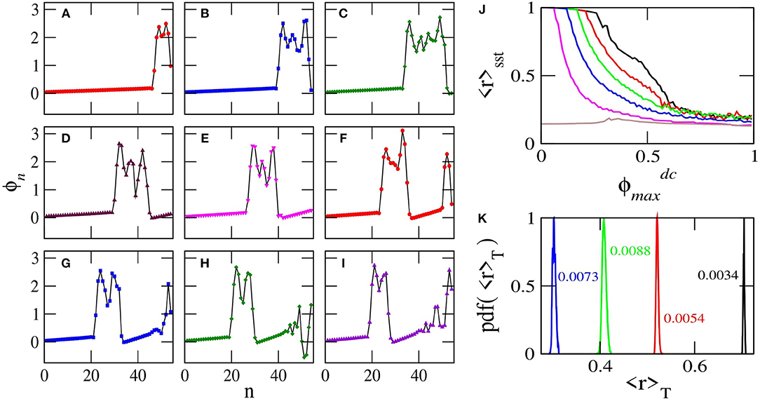
Figure 11. Flux profiles ϕ_n as a function of n for β_L = 0.86, γ = 0.01, λ = −0.02, N = 54, ϕ_ac = 0.04, Ω = 1.01, and (A) ${\varphi }_{max}^{dc}=0.25$; (B) 0.30; (C) 0.35; (D) 0.40; (E) 0.45; (F) 0.50; (G) 0.55; (H) 0.60; (I) 0.65. (J) The magnitude of the synchronization parameter averaged over the steady-state integration time 〈r〉_sst as a function of ${\varphi }_{max}^{dc}$ for the parameters of (A–I) but with ϕ_ac = 0.02 (black), 0.04 (red), 0.06 (green), 0.08 (blue), 0.10 (magenta), 0.12 (brown). (K) Distributions of the values of 〈r〉_T for ϕ_ac = 0.04, and ${\varphi }_{max}^{dc}=0.30$ (black), 0.40 (red), 0.50 (green), 0.60 (blue). The other parameters as in (A–I). The numbers next to the distributions are the corresponding full-width half-maximums.

Two typical “synchronization phase diagrams,” in which 〈r〉_sst is mapped on the ${\varphi }_{ac}-{\varphi }_{max}^{dc}$ parameter plane, are shown in Figures 12A,B for λ = −0.02 and λ = −0.06, respectively. The frequency of the driving ac field has been chosen once again to be very close to the geometrical resonance of a single SQUID oscillator, i.e., at Ω = 1.01. For each point on the ${\varphi }_{ac}-{\varphi }_{max}^{dc}$ plane, Equation (36) are integrated in time with a standard fourth order Runge-Kutta algorithm using the initial conditions of Equation (40), with a time-step h = 0.02. First, Equation (36) are integrated for 10⁵T time-units to eliminate transients, and then they are integrated for ${\tau }_{sst}=10^{5}T$ more time-units during which 〈r〉_sst is calculated. A comparison between Figures 12A,B reveals that the increase of the coupling strength between nearest-neighboring SQUIDs from λ = −0.02 to λ = −0.06 results in relatively moderate, quantitative differences only. In both Figures 12A,B, for values of ϕ_ac and ${\varphi }_{max}^{dc}$ in the red areas, the state of the SQUID metamaterial is synchronized. For values of ϕ_ac and ${\varphi }_{max}^{dc}$ in the dark-green, light-green and light-blue areas, the state of the SQUID metamaterial is either completely desynchronized, or a chimera state with one or more desynchronized clusters. In order to obtain more information about these states, additional measures should be used, such as the incoherence index S and the chimera index η.The definitions of these two measures follow closely those of previous works [90, 91], with the only difference being the choice of the relevant parameter on which subsequent calculations are performed. Specifically, here the time-derivative of the normalized fluxes through the loops of the SQUIDs, averaged over the driving period T, ${\langle {\dot{\varphi }}_n\rangle }_T(\tau )$, is chosen as the relevant variable. Note that a similar definition of the chimera index, using the magnitude of the synchronization (Kuramoto) parameter as the relevant variable, has been also proposed [88].

FIGURE 12

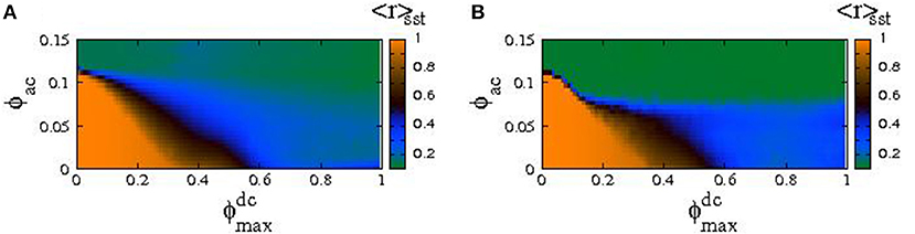
Figure 12. The magnitude of the synchronization parameter averaged over the steady-state integration time 〈r〉_sst mapped as a function of the ac flux amplitude and the maximum dc flux bias (${\varphi }_{ac}-{\varphi }_{max}^{dc}$ plane), for β_L = 0.86, γ = 0.01, N = 54, Ω = 1.01, and (A) λ = −0.02, (B) λ = −0.06.

The definitions for S and η employed here are as follows: First, define

$\begin{array}{ll}{v}_n(\tau )\equiv {\langle {\dot{\varphi }}_n\rangle }_T(\tau ),& (41)\end{array}$

where the angular brackets denote averaging over T, and

$\begin{array}{ll}{\bar{v}}_n(\tau )\equiv \frac{1}{n_0+1}{\displaystyle \sum _{j=n-n_0/2}^{n+n_0/2}}{v}_j(\tau ),& (42)\end{array}$

the local spatial average of v_n(τ) in a region of length n₀ + 1 around the site n at time τ (n₀ < N is an integer). Then, the local standard deviation of v_n(τ) is defined as

$\begin{array}{ll}{\sigma }_n(\tau )\equiv {\langle \sqrt{\frac{1}{n_0+1}{\displaystyle \sum _{j=n-n_0/2}^{n+n_0/2}{\left(v_j-{\overline{v}}_n\right)}^2}}\rangle }_{sst},& (43)\end{array}$

where the large angular brackets denote averaging over the steady-state integration time. The index of incoherence is then defined as

$\begin{array}{ll}S=1-\frac{1}{N}{\displaystyle \sum _{n=1}^N}{s}_n,& (44)\end{array}$

where s_n = Θ(δ − σ_n) with Θ being the Theta function, and δ a predefined threshold that is reasonably small. The index S takes its values in [0, 1], with 0 and 1 corresponding to synchronized and desynchronized states, respectively, while all other values between them indicate the existence of a chimera or multi-chimera state. Finally, the chimera index is defined as

$\begin{array}{ll}\eta ={\displaystyle \sum _{n=1}^N}|s_n-s_{n+1}|/2,& (45)\end{array}$

and takes positive integer values. The chimera index η gives the number of desynchronized clusters of a (multi-)chimera state, except in the case of a completely desynchronized state where it gives zero. In Figure 13, the incoherence index S and the chimera index η are mapped on the ${\varphi }_{ac}-{\varphi }_{max}^{dc}$ plane for the same parameters as in Figure 12A.

FIGURE 13

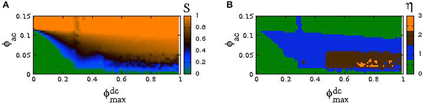
Figure 13. The index of incoherence S (A) and the chimera index η (B) are mapped on the ${\varphi }_{ac}-{\varphi }_{max}^{dc}$ plane, for the same parameters as in Figure 12A and n₀ = 4, δ = 10⁻⁴.

Figures 13A,B provide more information about the state of the SQUID metamaterial at a particular point on the ${\varphi }_{ac}-{\varphi }_{max}^{dc}$ plane. In Figure 13A, for values of ϕ_ac and ${\varphi }_{max}^{dc}$ in the light-green area (S = 0) the SQUID metamaterial is in a synchronized state (see the corresponding area in Figure 13B in which η = 0). For values of ϕ_ac and ${\varphi }_{max}^{dc}$ in the red area (S = 1), the SQUID metamaterial is completely desynchronized (the corresponding area in Figure 13B has η = 0 due to technical reasons). For values of ϕ_ac and ${\varphi }_{max}^{dc}$ in one of the other areas, the SQUID metamaterial is in a chimera state with one, two, or three desynchronized clusters, as it can be inferred from Figure 13B.

Using the combined information from Figures 12, 13, the form of the steady-state of a SQUID metamaterial can be predicted for any physically relevant value of ϕ_ac and ${\varphi }_{max}^{dc}$. In Figure 14, three flux profiles ϕ_n are shown as a function of n, along with the corresponding profiles of their time-derivatives, ${\dot{\varphi }}_n$. The profiles in Figures 14A–C, are obtained for ϕ_ac = 0.04 and ${\varphi }_{max}^{dc}=0.2$, 0.4, and 0.6, respectively, which are located in the light-green, light-blue, and dark-green area of Figure 14B. As it is expected, the state in Figure 14A is an almost synchronized one, in Figure 14B is a chimera state with one desynchronized cluster, while in Figure 14C is a chimera state with two desynchronized clusters. At this point, the use of the expression “almost synchronized” should be explained. In the presence of a dc flux gradient, it is impossible for a SQUID metamaterial to reach a completely synchronized state. This is because each SQUID is subject to a different dc flux, which modifies accordingly its resonance (eigen-)frequency. As a result, the flux oscillation amplitudes of the SQUIDs, whose oscillations are driven by the ac flux field of amplitude ϕ_ac and frequency Ω, are slightly different. On the other hand, the maximum of the flux oscillations for all the SQUIDs is attained at the same time. Indeed, as can be observed in Figure 14A. the flux profile ϕ_n is not horizontal, as it should be in the case of complete synchronization. Instead, that profile increases almost linearly from n = 1 to n = N (that increase is related to the dc flux gradient). However, the voltage profile ${\dot{\varphi }}_n$ is zero for any n, indicating that all the SQUID oscillators are in phase. Since, in such a state of the SQUID metamaterial there is phase synchronization but no amplitude synchronization, the synchronization is not complete. However, the value of 〈r〉_sst in such a state is in the worst case higher than 0.96 for moderately high values of ϕ_ac = 0.02−0.10 (Figure 11J), which is a very high degree of global synchronization. Furthermore, the synchronized clusters in the chimera state profiles in Figures 14B,C, whose length coincides with that of the horizontal segments of the $\dot{{\varphi }_n}$ profiles, also exhibit a very high degree of global synchronization (〈r〉_sst > 0.96).

FIGURE 14

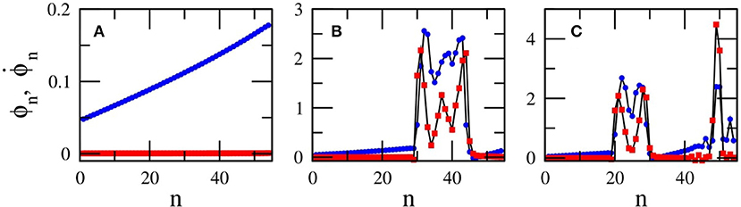
Figure 14. Flux and voltage profiles ϕ_n (blue) and $v_n={\dot{\varphi }}_n$ (red), respectively, as a function of n for β_L = 0.86, γ = 0.01, Ω = 1.01, ϕ_ac = 0.04, and (A) ${\varphi }_{max}^{dc}=0.2$, (B) ${\varphi }_{max}^{dc}=0.4$, (C) ${\varphi }_{max}^{dc}=0.6$.

4. Discussion

The emergence of chimera and multi-chimera states in a 1D SQUID metamaterial driven by an ac flux field is demonstrated numerically, using a well-established model that relies on equivalent electrical circuits. Chimera states may emerge both with local coupling between SQUID (nearest-neighbor coupling) and non-local coupling between SQUIDs which falls-off as the inverse cube of their center-to-center distance. A large variety of initial conditions can generate chimera states which persist for very long times. In the previous section, the expression “steady-state integration time” is used repeatedly; however, in some cases this may not be very accurate, since chimera states are generally metastable and sudden changes may occur at any instant of time-integration which results in sudden jumps the synchronization parameter 〈r〉_T [33]. For the chimera states presented here, however, no such sudden changes have been observed. Along with the ac flux field, a dc flux bias, the same at any SQUID, can be also applied to the 1D SQUID metamaterial. Chimera states can be generated in that case as well, although not shown here. Although a large volume of analytical and numerical studies on the existence and properties of chimera states for a variety of non-linear mathematical models of coupled oscillators exists, there are comparatively very few studies in which the oscillators are periodically (i.e., sinusoidally) driven. Some of the latter studies include an array of locally coupled bistable Duffing oscillators with a common sinusoidal forcing [92], in networks of non-locally coupled van der Pol-Duffing oscillators excited by a sinusoidal drive [93], and locally coupled extended Duffing oscillators with harmonic forcing [94].

The emergence of those counter-intuitive states, their form and their global degree of synchronization depends crucially on the initial conditions. If the SQUID metamaterial is initialized with zeros, the generation of chimera states does not seem to be possible for spatially constant dc flux bias ϕ_dc. In that case, synchronization-desynchronization and reverse synchronization-desynchronization transitions may occur by varying the ac flux amplitude ϕ_ac or the dc flux bias ϕ_dc. In the former transition, a completely synchronized state suddenly becomes a completely desynchronized one. The replacement of the spatially constant dc flux bias by a position-dependent one, ${\varphi }_n^{dc}$, makes possible the generation of chimera states from zero initial conditions. In the latter case, it is possible to generate chimera states whose characteristics depend on the external parameters, such as the dc flux gradient, and the amplitude and frequency of the ac flux field. Specifically, given that the SQUID metamaterial is initially “at rest” (${\varphi }_n(\tau =0)={\dot{\varphi }}_n(\tau =0)=0$ for any n), the values of the external parameters determine whether a chimera state will be generated, its degree of synchronization and its multiplicity, as well as the location and the size of its desynchronized cluster(s). It is in this sense that we use the term “controlled generation of chimera states” in the beginning of this section.

Here, the driving frequency is always chosen to be very close to the geometrical frequency of the individual SQUIDs. In the case of relatively strong non-linearity, considered here, the resonance frequency of individual SQUIDs is shifted to practically around the geometrical frequency. That is, for relatively strong non-linearity, the driving frequency was chosen so that the SQUIDs are at resonance. For a single SQUID driven close to its resonance, the relatively strong non-linearity makes it highly multistable; then, several stable and unstable single SQUID states may coexist (see the snake-like curves presented in section 2.1). This dynamic multistability effect is of major importance for the emergence of chimera states in SQUID metamaterials, as it is explained below.

The dynamic complexity of N SQUIDs which are coupled together increases with increasing N; this effect has been described in the past for certain arrays of coupled non-linear oscillators as attractor crowding [95, 96]. This complexity is visible already for two coupled SQUIDs, where the number of stable states close to the geometrical resonance increases more than two times compared to that of a single SQUID [34]; some of these states can even be chaotic. Interestingly, the existence of homoclinic chaos in a pair of coupled SQUIDs has been proved by analytical means [97, 98]. It has been argued that the number of stable limit cycles (i.e., periodic solutions) in such systems scales with the number of oscillators N as (N − 1)!. As a result, their basins of attraction crowd more and more tightly in phase space with increasing N. The multistability of individual SQUIDs around the resonance frequency enhances the attractor crowding effect in SQUID metamaterial. Apart from the large number of periodic solutions (limit cycles), a number of coexisting chaotic solutions may also appear as in the two-SQUID system. All these states are available for each SQUID to occupy. Then, with appropriate initialization of the SQUID metamaterial, or by applying a dc flux gradient to it, a number of SQUIDs that belong to the same cluster may occupy a chaotic state. The flux oscillations of these SQUIDs then generally differ in both their amplitude and phase, resulting for that cluster to be desynchronized. Alternatingly, a number of SQUIDs that belong to the same cluster may find themselves in a region of phase-space with a high density of periodic solutions. Then, the flux in these SQUID oscillators may jump irregularly from one periodic state to another resulting in effectively random dynamics and in effect for that cluster to be desynchronized. At the same time, the other cluster(s) of SQUIDs can remain synchronized and, as a result, a chimera state emerges.

Author Contributions

NL conceived the structure of the manuscript. JH and NL performed the simulations. All authors listed performed data analysis and have made intellectual contribution to the work, and approved it for publication.

Conflict of Interest Statement

The authors declare that the research was conducted in the absence of any commercial or financial relationships that could be construed as a potential conflict of interest.

Acknowledgments

This research has been financially supported by the General Secretariat for Research and Technology (GSRT) and the Hellenic Foundation for Research and Innovation (HFRI) (Code: 203).

References

1. Smith DR, Pendry JB, Wiltshire. Metamaterials and negative refractive index. Science (2004) 305:788–92. doi: 10.1126/science.1096796

PubMed Abstract | CrossRef Full Text | Google Scholar

2. Linden S, Enkrich C, Dolling G, Klein MW, Zhou J, Koschny T, et al. Photonic metamaterials: magnetism at optical frequencies. IEEE J Selec Top Quant Electron. (2006) 12:1097–105. doi: 10.1109/JSTQE.2006.880600

CrossRef Full Text | Google Scholar

3. Padilla WJ, Basov DN, Smith DR. Negative refractive index metamaterials. Mater Today. (2006) 9:28–35. doi: 10.1016/S1369-7021(06)71573-5

CrossRef Full Text | Google Scholar

4. Shalaev VM. Optical negative-index metamaterials. Nature Photon. (2007) 1:41–8. doi: 10.1038/nphoton.2006.49

CrossRef Full Text | Google Scholar

5. Litchinitser NM, Shalaev VM. Photonic metamaterials. Laser Phys Lett. (2008) 5:411–20. doi: 10.1002/lapl.200810015

CrossRef Full Text | Google Scholar

6. Soukoulis CM, Wegener M. Past achievements and future challenges in the development of three-dimensional photonic metamaterials. Nature Photon. (2011) 5:523–30. doi: 10.1038/nphoton.2011.154

CrossRef Full Text | Google Scholar

7. Liu Y, Zhang X. Metamaterials: a new frontier of science and technology. Chem Soc Rev. (2011) 40:2494–507. doi: 10.1039/c0cs00184h

PubMed Abstract | CrossRef Full Text | Google Scholar

8. Simovski CR, Belov PA, Atrashchenko AV, Kivshar YS. Wire metamaterials: physics and applications. Adv Mater. (2012) 24:4229–48. doi: 10.1002/adma.201200931

PubMed Abstract | CrossRef Full Text | Google Scholar

9. Engheta N, Ziolkowski RW. Metamaterials: Physics and Engineering Explorations. New Jersey, NJ: Wiley-IEEE Press (2006).

Google Scholar

10. Pendry JB. Fundamentals and Applications of Negative Refraction in Metamaterials. New Jersey, NY: Princeton University Press (2007).

Google Scholar

11. Ramakrishna SA, Grzegorczyk T. Physics and Applications of Negative Refractive Index Materials. New York, NY: SPIE and CRC Press (2009).

Google Scholar

12. Cui TJ, Smith DR, Liu R. Metamaterials Theory, Design and Applications. New York, NY: Springer (2010).

Google Scholar

13. Cai W, Shalaev V. Optical Metamaterials, Fundamentals and Applications. Heidelberg: Springer (2010).

Google Scholar

14. Solymar L, Shamonina E. Waves in Metamaterials. New York, NY: Oxford University Press (2009).

Google Scholar

15. Noginov MA, Podolskiy VA. Tutorials in Metamaterials. Boca Raton, FL: Taylor & Francis (2012).

Google Scholar

16. Tong XC. Functional Metamaterials and Metadevices, Springer Series in Materials Science, Vol. 262. Cham: Springer International Publishing AG (2018).

Google Scholar

17. Anlage SM. The physics and applications of superconducting metamaterials. J Opt. (2011) 13:024001–10. doi: 10.1088/2040-8978/13/2/024001

CrossRef Full Text | Google Scholar

18. Jung P, Ustinov AV, Anlage SM. Progress in superconducting metamaterials. Supercond Sci Technol. (2014) 27:073001. doi: 10.1088/0953-2048/27/7/073001

CrossRef Full Text | Google Scholar

19. Jin B, Zhang C, Engelbrecht S, Pimenov A, Wu J, Xu Q, et al. Low loss and magnetic field-tunable superconducting terahertz metamaterials. Opt Express. (2010) 18:17504–9. doi: 10.1364/OE.18.017504

CrossRef Full Text | Google Scholar

20. Zhang CH, Wu JB, Jin BB, Ji ZM, Kang L, Xu WW, et al. Low-loss terahertz metamaterial from superconducting niobium nitride films. Opt Express. (2012) 20:42–7. doi: 10.1364/OE.20.000042

PubMed Abstract | CrossRef Full Text | Google Scholar

21. Gu J, Singh R, Tian Z, Cao W, Xing Q, He MX, et al. Terahertz superconductor metamaterial. Appl Phys Lett. (2010) 97:071102. doi: 10.1063/1.3479909

CrossRef Full Text | Google Scholar

22. Zhang X, Gu J, Han J, Zhang W. Tailoring electromagnetic responses in terahertz superconducting metamaterials. Front Optoelectron. (2014) 8:44–56. doi: 10.1007/s12200-014-0439-x

CrossRef Full Text | Google Scholar

23. Du C, Chen H, Li S. Quantum left-handed metamaterial from superconducting quantum-interference devices. Phys Rev B. (2006) 74:113105–4. doi: 10.1103/PhysRevB.74.113105

CrossRef Full Text | Google Scholar

24. Lazarides N, Tsironis GP. RF superconducting quantum interference device metamaterials. Appl Phys Lett. (2007) 90:163501. doi: 10.1063/1.2722682

CrossRef Full Text | Google Scholar

25. Josephson B. Possible new effects in superconductive tunnelling. Phys Lett A. (1962) 1:251–5. doi: 10.1016/0031-9163(62)91369-0

CrossRef Full Text | Google Scholar

26. Butz S, Jung P, Filippenko LV, Koshelets VP, Ustinov AV. A one-dimensional tunable magnetic metamaterial. Opt Express. (2013) 21:22540–8. doi: 10.1364/OE.21.022540

PubMed Abstract | CrossRef Full Text | Google Scholar

27. Trepanier M, Zhang D, Mukhanov O, Anlage SM. Realization and modeling of RF superconducting quantum interference device metamaterials. Phys Rev X. (2013) 3:041029. doi: 10.1103/PhysRevX.3.041029

CrossRef Full Text | Google Scholar

28. Zhang D, Trepanier M, Mukhanov O, Anlage SM. Broadband transparency of macroscopic quantum superconducting metamaterials. Phys Rev X. (2015) 5:041045. doi: 10.1103/PhysRevX.5.041045

CrossRef Full Text | Google Scholar

29. Jung P, Butz S, Marthaler M, Fistul MV, Leppäkangas J, Koshelets VP, et al. Multistability and switching in a superconducting metamaterial. Nat Commun. (2014) 5:3730. doi: 10.1038/ncomms4730

PubMed Abstract | CrossRef Full Text | Google Scholar

30. Trepanier M, Zhang D, Mukhanov O, Koshelets VP, Jung P, Butz S, et al. Coherent oscillations of driven rf squid metamaterials. Phys Rev E. (2017) 95:050201. doi: 10.1103/PhysRevE.95.050201

PubMed Abstract | CrossRef Full Text | Google Scholar

31. Lazarides N, Tsironis GP, Eleftheriou M. Dissipative discrete breathers in RF squid metamaterials. Nonlinear Phenom Complex Syst. (2008) 11:250–8. Available online at: http://www.j-npcs.org/abstracts/vol2008/v11no2/v11no2p250.html

Google Scholar

32. Tsironis GP, Lazarides N, Margaris I. Wide-band tuneability, nonlinear transmission, and dynamic multistability in squid metamaterials. Appl Phys A. (2014) 117:579–88. doi: 10.1007/s00339-014-8706-7

CrossRef Full Text | Google Scholar

33. Lazarides N, Neofotistos G, Tsironis GP. Chimeras in squid metamaterials. Phys Rev B. (2015) 91:054303. doi: 10.1103/PhysRevB.91.054303

CrossRef Full Text | Google Scholar

34. Hizanidis J, Lazarides N, Tsironis GP. Robust chimera states in squid metamaterials with local interactions. Phys Rev E. (2016) 94:032219. doi: 10.1103/PhysRevE.94.032219

PubMed Abstract | CrossRef Full Text | Google Scholar

35. Hizanidis J, Lazarides N, Neofotistos G, Tsironis G. Chimera states and synchronization in magnetically driven squid metamaterials. Eur Phys J Spec Top. (2016) 225:1231–43. doi: 10.1140/epjst/e2016-02668-9

CrossRef Full Text | Google Scholar

36. Lazarides N, Tsironis GP. Superconducting metamaterials. Phys Rep. (2018) 752:1–67. doi: 10.1016/j.physrep.2018.06.005

CrossRef Full Text | Google Scholar

37. Kuramoto Y, Battogtokh D. Coexistence of coherence and incoherence in nonlocally coupled phase oscillators. Nonlinear Phenom Complex Syst. (2002) 5:380–5. Available online at: http://www.j-npcs.org/online/vol2002/v5no4/v5no4p380.pdf

Google Scholar

38. Panaggio MJ, Abrams DM. Chimera states: coexistence of coherence and incoherence in network of coulped oscillators. Nonlinearity. (2015) 28:R67–87. doi: 10.1088/0951-7715/28/3/R67

CrossRef Full Text | Google Scholar

39. Schöll E. Synchronization patterns and chimera states in complex networks: interplay of topology and dynamics. Eur Phys J Spec Top. (2016) 225:891–919. doi: 10.1140/epjst/e2016-02646-3

CrossRef Full Text | Google Scholar

40. Yao N, Zheng Z. Chimera states in spatiotemporal systems: theory and applications. Int J Mod Phys B. (2016) 30:1630002. doi: 10.1142/S0217979216300024

CrossRef Full Text | Google Scholar

41. Abrams DM, Strogatz SH. Chimera states for coupled oscillators. Phys Rev Lett. (2004) 93:174102. doi: 10.1103/PhysRevLett.93.174102

PubMed Abstract | CrossRef Full Text | Google Scholar

42. Kuramoto Y, Shima SI, Battogtokh D, Shiogai Y. Mean-field theory revives in self-oscillatory fields with non-local coupling. Prog Theor Phys Suppl. (2006) 161:127–43. doi: 10.1143/PTPS.161.127

CrossRef Full Text | Google Scholar

43. Omel'chenko OE, Maistrenko YL, Tass PA. Chimera states: the natural link between coherence and incoherence. Phys Rev Lett. (2008) 100:044105. doi: 10.1103/PhysRevLett.100.044105

PubMed Abstract | CrossRef Full Text | Google Scholar

44. Abrams DM, Mirollo R, Strogatz SH, Wiley DA. Solvable model for chimera states of coupled oscillators. Phys Rev Lett. (2008) 101:084103. doi: 10.1103/PhysRevLett.101.084103

PubMed Abstract | CrossRef Full Text | Google Scholar

45. Pikovsky A, Rosenblum M. Partially integrable dynamics of hierarchical populations of coupled oscillators. Phys Rev Lett. (2008) 101:264103. doi: 10.1103/PhysRevLett.101.264103

PubMed Abstract | CrossRef Full Text | Google Scholar

46. Ott E, Antonsen TM. Long time evolution of phase oscillator systems. Chaos. (2009) 19:023117. doi: 10.1063/1.3136851

PubMed Abstract | CrossRef Full Text | Google Scholar

47. Martens EA, Laing CR, Strogatz SH. Solvable model of spiral wave chimeras. Phys Rev Lett. (2010) 104:044101. doi: 10.1103/PhysRevLett.104.044101

PubMed Abstract | CrossRef Full Text | Google Scholar

48. Omelchenko I, Maistrenko Y, Hövel P, Schöll E. Loss of coherence in dynamical networks: spatial chaos and chimera states. Phys Rev Lett. (2011) 106:234102. doi: 10.1103/PhysRevLett.106.234102

PubMed Abstract | CrossRef Full Text | Google Scholar

49. Yao N, Huang ZG, Lai YC, Zheng ZG. Robustness of chimera states in complex dynamical systems. Sci Rep. (2013) 3:3522. doi: 10.1038/srep03522

PubMed Abstract | CrossRef Full Text | Google Scholar

50. Omelchenko I, Omel'chenko OE, Hövel P, Schöll E. When nonlocal coupling between oscillators becomes stronger: matched synchrony or multichimera states. Phys Rev Lett. (2013) 110:224101. doi: 10.1103/PhysRevLett.110.224101

CrossRef Full Text | Google Scholar

51. Hizanidis J, Kanas V, Bezerianos A, Bountis T. Chimera states in networks of nonlocally coupled hindmarsh-rose neuron models. Int J Bifurcation Chaos. (2014) 24:1450030. doi: 10.1142/S0218127414500308

CrossRef Full Text | Google Scholar

52. Zakharova A, Kapeller M, Schöll E. Chimera death: symmetry breaking in dynamical networks. Phys Rev Lett. (2014) 112:154101. doi: 10.1103/PhysRevLett.112.154101

PubMed Abstract | CrossRef Full Text | Google Scholar

53. Bountis T, Kanas V, Hizanidis J, Bezerianos A. Chimera states in a two-population network of coupled pendulum-like elements. Eur Phys J Spec Top. (2014) 223:721–8. doi: 10.1140/epjst/e2014-02137-7

CrossRef Full Text | Google Scholar

54. Yeldesbay A, Pikovsky A, Rosenblum M. Chimeralike states in an ensemble of globally coupled oscillators. Phys Rev Lett. (2014) 112:144103. doi: 10.1103/PhysRevLett.112.144103

PubMed Abstract | CrossRef Full Text | Google Scholar

55. Haugland SW, Schmidt L, Krischer K. Self-organized alternating chimera states in oscillatory media. Sci Rep. (2015) 5:9883. doi: 10.1038/srep09883

PubMed Abstract | CrossRef Full Text | Google Scholar

56. Bera BK, Ghosh D, Lakshmanan M. Chimera states in bursting neurons. Phys Rev E. (2016) 93:012205. doi: 10.1103/PhysRevE.93.012205

PubMed Abstract | CrossRef Full Text | Google Scholar

57. Shena J, Hizanidis J, Kovanis V, Tsironis GP. Turbulent chimeras in large semiconductor laser arrays. Sci Rep. (2017) 7:42116. doi: 10.1038/srep42116

PubMed Abstract | CrossRef Full Text | Google Scholar

58. Sawicki J, Omelchenko I, Zakharova A, Schöll E. Chimera states in complex networks: interplay of fractal topology and delay. Eur Phys J Spec Top. (2017) 226:1883–92. doi: 10.1140/epjst/e2017-70036-8

CrossRef Full Text | Google Scholar

59. Ghosh S, Jalan S. Engineering chimera patterns in networks using heterogeneous delays. Chaos. (2018) 28:071103. doi: 10.1063/1.5042133

PubMed Abstract | CrossRef Full Text | Google Scholar

60. Shepelev IA, Vadivasova TE. Inducing and destruction of chimeras and chimera-like states by an external harmonic force. Phys Lett A. (2018) 382:690–6. doi: 10.1016/j.physleta.2017.12.055

CrossRef Full Text | Google Scholar

61. Banerjee A, Sikder D. Transient chaos generates small chimeras. Phys Rev E. (2018) 98:032220. doi: 10.1103/PhysRevE.98.032220

CrossRef Full Text | Google Scholar

62. Tinsley MR, Nkomo S, Showalter K. Chimera and phase-cluster states in populations of coupled chemical oscillators. Nat Phys. (2012) 8:662–5. doi: 10.1038/nphys2371

CrossRef Full Text | Google Scholar

63. Hagerstrom AM, Murphy TE, Roy R, Hövel P, Omelchenko I, Schöll E. Experimental observation of chimeras coulped-map lattices. Nat Phys. (2012) 8:658–61. doi: 10.1038/nphys2372

CrossRef Full Text | Google Scholar

64. Wickramasinghe M, Kiss IZ. Spatially organized dynamical states in chemical oscillator networks: synchronization, dynamical differentiation, and chimera patterns. PLoS ONE (2013) 8:e80586. doi: 10.1371/journal.pone.0080586

PubMed Abstract | CrossRef Full Text | Google Scholar

65. Nkomo S, Tinsley MR, Showalter K. Chimera states in populations of nonlocally coupled chemical oscillators. Phys Rev Lett. (2013) 110:244102. doi: 10.1103/PhysRevLett.110.244102

PubMed Abstract | CrossRef Full Text | Google Scholar

66. Martens EA, Thutupalli S, Fourriére A, Hallatschek O. Chimera states in mechanical oscillator networks. Proc Natl Acad Sci USA. (2013) 110:10563–7. doi: 10.1073/pnas.1302880110

PubMed Abstract | CrossRef Full Text | Google Scholar

67. Schönleber K, Zensen C, Heinrich A, Krischer K. Patern formation during the oscillatory photoelectrodissolution of n-type silicon: turbulence, clusters and chimeras. New J Phys. (2014) 16:063024. doi: 10.1088/1367-2630/16/6/063024

CrossRef Full Text | Google Scholar

68. Viktorov EA, Habruseva T, Hegarty SP, Huyet G, Kelleher B. Coherence and incoherence in an optical comb. Phys Rev Lett. (2014) 112:224101. doi: 10.1103/PhysRevLett.112.224101

PubMed Abstract | CrossRef Full Text | Google Scholar

69. Rosin DP, Rontani D, Haynes ND, Schöll E, Gauthier DJ. Transient scaling and resurgence of chimera states in coupled boolean phase oscillators. Phys Rev E. (2014) 90:030902. doi: 10.1103/PhysRevE.90.030902

CrossRef Full Text | Google Scholar

70. Schmidt L, Schönleber K, Krischer K, García-Morales V. Coexistence of synchrony and incoherence in oscillatory media under nonlinear global coupling. Chaos. (2014) 24:013102. doi: 10.1063/1.4858996

PubMed Abstract | CrossRef Full Text | Google Scholar

71. Gambuzza LV, Buscarino A, Chessari S, Fortuna L, Meucci R, Frasca M. Experimental investigation of chimera states with quiescent and synchronous domains in coupled electronic oscillators. Phys Rev E. (2014) 90:032905. doi: 10.1103/PhysRevE.90.032905

PubMed Abstract | CrossRef Full Text | Google Scholar

72. Kapitaniak T, Kuzma P, Wojewoda J, Czolczynski K, Maistrenko Y. Imperfect chimera states for coupled pendula. Sci Rep. (2014) 4:6379. doi: 10.1038/srep06379

PubMed Abstract | CrossRef Full Text | Google Scholar

73. Larger L, Penkovsky B, Maistrenko Y. Laser chimeras as a paradigm for multistable patterns in complex systems. Nat Comms. (2015) 6:7752. doi: 10.1038/ncomms8752

PubMed Abstract | CrossRef Full Text | Google Scholar

74. Hart JD, Bansal K, Murphy TE, Roy R. Experimental observation of chimera and cluster states in a minimal globally coupled network. Chaos. (2016) 26:094801. doi: 10.1063/1.4953662

PubMed Abstract | CrossRef Full Text | Google Scholar

75. English LQ, Zampetaki A, Kevrekidis PG, Skowronski K, Fritz CB, Abdoulkary S. Analysis and observation of moving domain fronts in a ring of coupled electronic self-oscillators. Chaos. (2017) 27:103125. doi: 10.1063/1.5009088

PubMed Abstract | CrossRef Full Text | Google Scholar

76. Totz JF, Rode J, Tinsley MR, Showalter K, Engel H. Spiral wave chimera states in large populations of coupled chemical oscillators. Nat Phys. (2018) 14:282–5. doi: 10.1038/s41567-017-0005-8

CrossRef Full Text | Google Scholar

77. Clarke J, Braginski AI. The SQUID Handbook Vol. I: Fundamentals and Technology of SQUIDs and SQUID Systems. Weinheim: Wiley-VCH (2004).

Google Scholar

78. Clarke J, Braginski AI. The SQUID Handbook Vol. II: Applications of SQUIDs and SQUID Systems. Weinheim: Wiley-VCH (2004).

Google Scholar

79. Hizanidis J, Lazarides N, Tsironis GP. Flux bias-controlled chaos and extreme multistability in squid oscillators. Chaos. (2018) 28:063117. doi: 10.1063/1.5020949

PubMed Abstract | CrossRef Full Text | Google Scholar

80. Likharev KK. Dynamics of Josephson Junctions and Circuits. Philadelphia, PA: Gordon and Breach (1986).

Google Scholar

81. Swift JW, Wiesenfeld K. Suppression of period doubling in symmetric systems. Phys Rev Lett. (1984) 52:705. doi: 10.1103/PhysRevLett.52.705

CrossRef Full Text | Google Scholar

82. Flach S, Gorbach AV. Discrete breathers–advances in theory and applications. Phys Rep. (2008) 467:1–116. doi: 10.1016/j.physrep.2008.05.002

CrossRef Full Text | Google Scholar

83. Flach S, Gorbach A. Discrete breathers with dissipation. Lect Notes Phys. (2008) 751:289–320. doi: 10.1007/978-3-540-78217-9_11

CrossRef Full Text | Google Scholar

84. Tsironis GP, Lazarides N, Eleftheriou M. Dissipative breathers in rf squid metamaterials. PIERS Online. (2009) 5:26–30. doi: 10.2529/PIERS081006095539

CrossRef Full Text | Google Scholar

85. Lazarides N, Tsironis GP. Intrinsic localization in nonlinear and superconducting metamaterials. Proc SPIE. (2012) 8423:84231K. doi: 10.1117/12.922708

CrossRef Full Text | Google Scholar

86. Lazarides N, Tsironis GP. Nonlinear localization in metamaterials. In: Shadrivov I, Lapine M, Kivshar YS, editors. Nonlinear, Tunable and Active Metamaterials. Cham: Springer International Publishing (2015). p. 281–301.

Google Scholar

87. Lazarides N, Tsironis GP. Multistable dissipative breathers and collective states in squid lieb metamaterials. Phys Rev E. (2018) 98:012207. doi: 10.1103/PhysRevE.98.012207

PubMed Abstract | CrossRef Full Text | Google Scholar

88. Shanahan M. Metastable chimera states in community-structured oscillator networks. Chaos. (2010) 20:013108. doi: 10.1063/1.3305451

PubMed Abstract | CrossRef Full Text | Google Scholar

89. Wildie M, Shanahan M. Metastability and chimera states in modular delay and pulse-coupled oscillator networks. Chaos. (2012) 22:043131. doi: 10.1063/1.4766592

PubMed Abstract | CrossRef Full Text | Google Scholar

90. Gopal R, Chandrasekar VK, Venkatesan A, Lakshmanan M. Observation and characterization of chimera states in coupled dynamical systems with nonlocal coupling. Phys Rev E. (2014) 89:052914. doi: 10.1103/PhysRevE.89.052914

PubMed Abstract | CrossRef Full Text | Google Scholar

91. Gopal R, Chandrasekar VK, Venkatesan A, Lakshmanan M. Chimera at the phase-flip transition of an ensemble of identical nonlinear oscillators. Commun Nonlinear Sci Numer Simulat. (2018) 59:30–46. doi: 10.1016/j.cnsns.2017.11.005

CrossRef Full Text | Google Scholar

92. Chandrasekar VK, Suresh R, Senthilkumar DV, Lakshmanan M. Coexisting coherent and incoherent domains near saddle-node bifurcation. EPL. (2015) 111:60008. doi: 10.1209/0295-5075/111/60008

CrossRef Full Text | Google Scholar

93. Dudkowski D, Maistrenko Yu, Kapitaniak T. Occurrence and stability of chimera states in coupled externally excited oscillators. Chaos. (2016) 26:116306. doi: 10.1063/1.4967386

PubMed Abstract | CrossRef Full Text | Google Scholar

94. Clerc MG, Coulibaly S, Ferré MA, Rojas RG. Chimera states in a Duffing oscillators chain coupled to nearest neighbors. Chaos. (2018) 28:083126. doi: 10.1063/1.5025038

PubMed Abstract | CrossRef Full Text | Google Scholar

95. Wiesenfeld K, Hadley P. Attractor crowding in oscillator arrays. Phys Rev Lett. (1989) 62:1335–8. doi: 10.1103/PhysRevLett.62.1335

PubMed Abstract | CrossRef Full Text | Google Scholar

96. Tsang KY, Wiesenfeld K. Attractor crowding in josephson junction arrays. Appl Phys Lett. (1990) 56:495–7. doi: 10.1063/1.102774

CrossRef Full Text | Google Scholar

97. Agaoglou M, Rothos VM, Susanto H. Homoclinic chaos in a pair of parametrically-driven coupled squids. J Phys Conf Series. (2015) 574:012027. doi: 10.1088/1742-6596/574/1/012027

CrossRef Full Text | Google Scholar

98. Agaoglou M, Rothos VM, Susanto H. Homoclinic chaos in coupled squids. Chaos Solit Fract. (2017) 99:133–40. doi: 10.1016/j.chaos.2017.04.003

CrossRef Full Text | Google Scholar