 Zhiyong Zhou
 Jun Yu
94% of researchers rate our articles as excellent or good
Learn more about the work of our research integrity team to safeguard the quality of each article we publish.
Find out more
ORIGINAL RESEARCH article
Front. Appl. Math. Stat., 14 March 2019
Sec. Mathematics of Computation and Data Science
Volume 5 - 2019 | https://doi.org/10.3389/fams.2019.00014
This article is part of the Research TopicRecent Developments in Signal Approximation and ReconstructionView all 6 articles
As an extension of the widely used ℓr-minimization with 0 < r ≤ 1, a new non-convex weighted ℓr − ℓ1 minimization method is proposed for compressive sensing. The theoretical recovery results based on restricted isometry property and q-ratio constrained minimal singular values are established. An algorithm that integrates the iteratively reweighted least squares algorithm and the difference of convex functions algorithm is given to approximately solve this non-convex problem. Numerical experiments are presented to illustrate our results.
Compressive sensing (CS) has attracted a great deal of interests since its advent [1, 2], see the monographs [3, 4] and the references therein for a comprehensive view. Basically, the goal of CS is to recover an unknown (approximately) sparse signal x ∈ ℝN from the noisy underdetermined linear measurements
with m ≪ N, A ∈ ℝm×N being the pre-given measurement matrix and e ∈ ℝm being the noise vector. If the measurement matrix A satisfies some kinds of incoherence conditions (e.g., mutual coherence condition [5, 6], restricted isometry property (RIP) [7, 8], null space property (NSP) [9, 10], or constrained minimal singular values (CMSV) [11, 12]), then stable (w.r.t. sparsity defect) and robust (w.r.t. measurement error) recovery results can be guaranteed by using the constrained ℓ1-minimization [13]:
Here the ℓ1-minimization problem works as a convex relaxation of ℓ0-minimization problem, which is NP-hard to solve [14].
Meanwhile, non-convex recovery algorithms such as the ℓr-minimization (0 < r < 1) have been proposed to enhance sparsity [15–20]. ℓr-minimization enables one to reconstruct the sparse signal from fewer number of measurements compared to the convex ℓ1-minimization, although it is more challenging to solve because of its non-convexity. Fortunately, an iteratively reweighted least squares (IRLS) algorithm can be applied to approximately solve this non-convex problem in practice [21, 22].
As an extension of the ℓr-minimization, we study in this paper the following weighted ℓr − ℓ1 minimization problem for sparse signal recovery:
where y = Ax + e with ∥e∥2 ≤ η, 0 ≤ α ≤ 1, and 0 < r ≤ 1. Throughout the paper, we assume that α ≠ 1 when r = 1. Obviously, it reduces to the traditional ℓr-minimization problem when α = 0. This hybrid norm model is inspired by the non-convex Lipschitz continuous ℓ1 − ℓ2 model (minimizing the difference of ℓ1 norm and ℓ2 norm) proposed in Lou et al. [23] and Yin et al. [24], which improves the ℓ1-minimization in a robust manner, especially for the highly coherent measurement matrices. Roughly speaking, the underlying logic of adopting these kinds of norm differences or the ratios of norms [25] comes from the fact that they can be viewed as sparsity measures, see the effective sparsity measure called q-ratio sparsity (involving the ratio of ℓ1 norm and ℓq norm) defined later in Definition 2 of section 2.2. Other recent related literatures include [26–29], to name a few.
To illustrate these weighted ℓr − ℓ1 norms (), we present their corresponding contour plots in Figure 11. As is shown, different non-convex patterns arise while varying the difference weight α or the norm order r. And the level curves of weighted ℓr − ℓ1 norms approach the x and y axes as the norm values get small, which reflects their ability to promote sparsity. In the present paper, we shall focus on both the theoretical aspects and the computational study for this non-convex sparse recovery method.
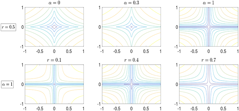
Figure 1. The contour plots for weighted ℓr − ℓ1 norms with different α and r. The first row corresponds to the cases that r = 0.5 with different α = 0, 0.3, 1, while the second row shows the cases that r = 0.1, 0.4, 0.7 with fixed α = 1.
This paper is organized as follows. In section 2, we derive the theoretical performance bounds for the weighted ℓr − ℓ1 minimization based on both r-RIP and q-ratio CMSV. In section 3, we give an algorithm to approximately solve the unconstrained version of the weighted ℓr − ℓ1 minimization problem. Numerical experiments are provided in section 4. Section 5 concludes with a brief summary and an outlook on future extensions.
In this section, we establish the theoretical performance bounds for the reconstruction error of the weighted ℓr − ℓ1 minimization problem, based on both r-RIP and q-ratio CMSV. Hereafter, we say a signal x ∈ ℝN is s-sparse if , and denote by xS the vector that coincides with x on the indices in S ⊆ [N]: = {1, 2, ⋯ , N} and takes zero outside S.
We start with the definition of the s-th r-restricted isometry constant, which was introduced in Chartrand and Staneva [30].
Definition 1. ([30]) For integer s > 0 and 0 < r ≤ 1, the s-th r-restricted isometry constant (RIC) δs = δs(A) of a matrix A ∈ ℝm×N is defined as the smallest δ ≥ 0 such that
for all s-sparse vectors x ∈ ℝN.
Then, the r-RIP means that the s-th r-RIC δs is small for reasonably large s. In Chartrand and Staneva [30], the authors established the recovery analysis result for ℓr-minimization problem based on this r-RIP. To extend this to the weighted ℓr − ℓ1 minimization problem, the following lemma plays a crucial role.
Lemma 1. Suppose x ∈ ℝN, 0 ≤ α ≤ 1 and 0 < r ≤ 1, then we have
In particular, when S = supp(x) ⊆ [N] and |S| = s, then
Proof. The right hand side of (5) follows immediately from the norm inequality for any x ∈ ℝN and 0 < r ≤ 1. As for the left hand side, it holds trivially if mini∈[N] |xi| = 0. When mini∈[N] |xi| ≠ 0, by dividing (mini∈[N] |xi|)r on both sides, it is equivalent to show that
By denoting , we have aj ≥ 1 for any 1 ≤ j ≤ N, and to show (7) it suffices to show
Assume the function . Then, as a result of
we have . Thus, the left hand side of (5) holds and the proof is completed. (6) follows as we apply (5) to xS.
Now, we are ready to present the r-RIP based bound for the ℓ2 norm of the reconstruction error.
Theorem 1. Let the ℓr-error of best s-term approximation of x be . We assume that a > 0 is properly chosen so that as is an integer. If
and suppose the measurement matrix A satisfies the condition
then any solution to the minimization problem (3) obeys
with and .
Proof. We assume that S is the index set that contains the largest s absolute entries of x so that and let . Then we have
which implies
Using the Holder's inequality, we obtain
By ∥Ax − y∥2 = ∥e∥2 ≤ η and the triangular inequality,
Thus,
Arrange , where S1 is the index set of M = as largest absolute entries of h in Sc, S2 is the index set of M largest absolute entries of h in , etc. And we denote S0 = S∪S1. Then, by adopting Lemma 1, for each i ∈ Sk, k ≥ 2,
Thus we have . Hence it follows that
Note that
therefore, with (11), it holds that
Meanwhile, according to the definition of r-RIC, we have
Thus by using (16), it follows that
where . Therefore, if δM + bδM+s < b − 1, then it yields that
On the other hand,
Since for any v1, v2 ≥ 0, combining (17) and (18) gives
The proof is completed.
Based on this theorem, we can obtain the following corollary by assuming that the original signal x is s-sparse (σs(x)r = 0) and the measurement vector is noise free (e = 0 and η = 0), which acts as a natural generalization of Theorem 2.4 in Chartrand and Staneva [30] from the case α = 0 to any α ∈ [0, 1].
Corollary 1. For any s-sparse signal x, if the conditions in Theorem 1 hold, then the unique solution of (3) with η = 0 is exactly x.
Remarks. Observe that r-RIP based condition for exact sparse recovery given in Chartrand and Staneva [30] reads
while ours goes to
with when α ∈ (0, 1]. Thus, the sufficient condition established here is slightly stronger than that for the traditional ℓr-minimization in Chartrand and Staneva [30] if α ∈ (0, 1].
Before the discussion of q-ratio CMSV, we start with presenting the definition of q-ratio sparsity as a kind of effective sparsity measure. We list the detailed statement here for the sake of completeness.
Definition 2. ([12, 31, 32]) For any non-zero z ∈ ℝN and non-negative q ∉ {0, 1, ∞}, the q-ratio sparsity level of z is defined as
The cases of q ∈ {0, 1, ∞}are evaluated as limits: , , and , where π(z) ∈ ℝN with entries πi(z) = |zi|/∥z∥1 and H1 is the ordinary Shannon entropy .
We are able to establish the performance bounds for both the ℓq norm and ℓr norm of the reconstruction error via a recently developed computable incoherence measure of the measurement matrix, called q-ratio CMSV. Its definition is given as follows.
Definition 3. ([12, 32]) For any real number s ∈ [1, N], q ∈ (1, ∞], and matrix A ∈ ℝm×N, the q-ratio constrained minimal singular value (CMSV) of A is defined as
Then, when the signal is exactly sparse, we have the following q-ratio CMSV based sufficient condition for valid upper bounds of the reconstruction error, which are much more concise to obtain than the r-RIP based ones.
Theorem 2. For any 1 < q ≤ ∞, 0 ≤ α ≤ 1, and 0 < r ≤ 1, if the signal x is s-sparse and the measurement matrix A satisfies the condition
then any solution to the minimization problem (3) obeys
Proof. Suppose the support of x to be S with |S| ≤ s and , then, based on (11), we have
Hence, for any 1 < q ≤ ∞, it holds that
Then since , it implies that . As a consequence,
Therefore, according to the definition of q-ratio CMSV the condition (22), and the fact that ∥Ah∥2 ≤ 2η [see (12)], we can obtain that
which completes the proof of (23). In addition, yields
Therefore, (24) holds and the proof is completed.
Remarks. Note that the results (11) and (12) in Theorem 1 of Zhou and Yu [12] correspond to the special case of α = 0 and r = 1 in this result. As a by-product of this theorem, we have that the perfect recovery can be guaranteed for any s-sparse signal x via (3) with η = 0, if there exists some q ∈ (1, ∞] such that the q-ratio CMSV of the measurement matrix A fulfils . As studied in Zhou and Yu [12, 32], this kind of q-ratio CMSV based sufficient conditions holds with high probability for subgaussian and a class of structured random matrices as long as the number of measurements is reasonably large.
Next, we extend the result to the case that x is compressible (i.e., not exactly sparse but can be well-approximated by an exactly sparse signal).
Theorem 3. For any 1 < q ≤ ∞, 0 ≤ α ≤ 1 and 0 < r ≤ 1, if the measurement matrix A satisfies the condition
then any solution to the minimization problem (3) fulfils
Proof. We assume that S is the index set that contains the largest s absolute entries of x so that and let . Then we still have (11), that is,
As a result,
holds for any 1 < q ≤ ∞, 0 ≤ α ≤ 1 and 0 < r ≤ 1.
To prove (30), we assume h ≠ 0 and , otherwise it holds trivially. Then
which implies that . Then combining with (33), it yields that
Therefore, we have
which completes the proof of (30).
Moreover, by using (33) and the inequality for any v1, v2 ≥ 0, we obtain that
Hence, (31) holds and the proof is completed.
Remarks. When we select α = 0 and r = 1, our results reduce to the corresponding results for the ℓ1-minimization or Basis Pursuit in Theorem 2 of Zhou and Yu [12]. In general, the sufficient condition provided here and that in Theorem 2 are slightly stronger than those established for the ℓ1-minimization in Zhou and Yu [12], noticing that and for any 1 < q ≤ ∞, 0 ≤ α ≤ 1, and 0 < r ≤ 1. This is caused by the fact that the technical inequalities used like (25) and (32) are far from tight. And this is also the case in the r-RIP based analysis. In fact, both r-RIP and q-ratio CMSV based conditions are loose. The discussion on much tighter sufficient conditions such as the NSP based conditions investigated in Tran and Webster [33], is left for future work.
In this section, we discuss the computational approach for the unconstrained version of (3), i.e.,
with λ > 0 being the regularizer parameter.
We integrate the iteratively reweighted least squares (IRLS) algorithm [21, 22] and the difference of convex functions algorithm (DCA) [34, 35] to solve this problem. In the outer loop, we use the IRLS to approximate the term , and use an iteratively reweighted ℓ1 norm to approximate . Specifically, we begin with and ε0 = 1, for n = 0, 1, ⋯ ,
where and . We let εn+1 = εn/10 if the error . The algorithm is stopped when for some n.
As for the inner loop used to solve (38), we view it as a minimization problem of a difference of two convex functions, that is, the objective function . We start with xn+1,0 = 0. For k = 0, 1, 2, ⋯ , in the k + 1 step, by linearizing H(x) with the approximation H(xn+1,k) + 〈yn+1,k, x − xn+1,k〉 where yn+1,k ∈ ∂H(xn+1,k), i.e. yn+1,k is a subgradient of H(x) at xn+1,k. Then we have
where sign(·) is the sign function. The termination criterion for the inner loop is set to be
for some given parameter tolerance parameter δ > 0. Basically, this algorithm can be regarded as a generalized version of IRLS algorithm. Obviously, when α = 0, it exactly reduces to the traditional IRLS algorithm used for solving the ℓr-minimization problem.
In this section, some numerical experiments on the proposed algorithm in section 3 are conducted to illustrate the performance of the weighted ℓr − ℓ1 minimization in simulated sparse signal recovery.
First, we focus on the weighted ℓr − ℓ1 minimization itself. In this set of experiments, the s-sparse signal x is of length N = 256, which is generated by choosing s entries uniformly at random, and then choosing the non-zero values from the standard normal distribution for these s entries. The underdetermined linear measurements y = Ax + e ∈ ℝm, where A ∈ ℝm×N is a standard Gaussian random matrix and the entries of the noise vector . Here we fix the number of measurements m = 64 and select a sequence of s as 10, 12, ⋯ , 36. We run the experiments for both noiseless and noisy cases. In all the experiments, we let the tolerance parameter δ = 10−3. And all the results are averaged over 100 repetitions.
In the noiseless case, i.e., σ = 0, we set λ = 10−6. In Figure 2, we show the results of successful recovery rate for different α (i.e., α = 0, 0.2, 0.5, 0.8, 1) while fixing r but varying the sparsity level s. We view it as a successful recovery if . We do the experiments for r = 0.3 and r = 0.7, respectively. As we can see, when r is fixed, the influence of the weight α is negligible, especially in the case that r is relatively small. But the performance does improve in some scenarios when a proper weight α is used. However, the problem of adaptively selecting the optimal α seems to be challenging and is left for future work. In addition, we present the reconstruction performances for different r (i.e., r = 0.01, 0.2, 0.5, 0.8, 1) while the weight α is fixed to be 0.2 and 0.8 in Figure 3. Note that small r is favored when the weight α is fixed. And a non-convex recovery with 0 < r < 1 performs much better than the convex case (r = 1).
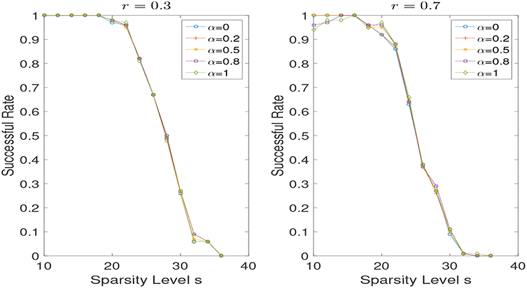
Figure 2. Successful recovery rate for different α with r = 0.3 and r = 0.7 in the noise free case, while varying the sparsity level s.
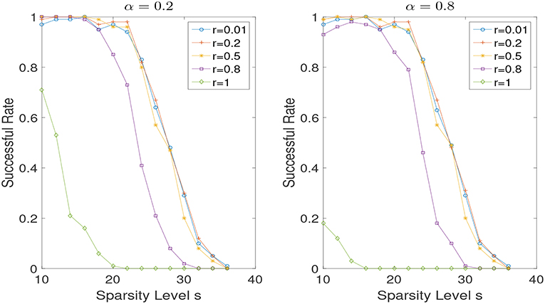
Figure 3. Successful recovery rate for different r with α = 0.2 and α = 0.8 in the noise free case, while varying the sparsity level s.
Next, we consider the noisy case, that is σ = 0.01. We set λ = 10−4. And we evaluate the recovery performance by the signal to noise ratio (SNR), which is given by
As shown in Figures 4, 5, the findings aforementioned can still be seen here.
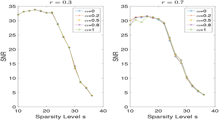
Figure 4. SNR for different α with r = 0.3 and r = 0.7 in the noisy case, while varying the sparsity level s.
Figure 5. SNR for different r with α = 0.2 and α = 0.8 in the noisy case, while varying the sparsity level s.
Second, we compare the weighted ℓr − ℓ1 minimization with some well-known algorithms. The following state-of-the-art recovery algorithms are operated:
• ADMM-Lasso, see Boyd et al. [36].
• CoSaMP, see Needell and Tropp [37].
• Iterative Hard Thresholding (IHT), see Blumensath and Davies [38].
• ℓ1 − ℓ2 minimization, see Yin et al. [24].
The tuning parameters used for these algorithms are the same as those adopted in section 5.2 of Yin et al. [24]. Specifically, for ADMM-Lasso, we choose λ = 10−6, β = 1, ρ = 10−5, εabs = 10−7, εrel = 10−5, and the maximum number of iterations maxiter = 5,000. For CoSaMP, maxiter=50 and the tolerance is set to be 10−8. The tolerance for IHT is 10−12. For ℓ1 − ℓ2 minimization, we choose the parameters as εabs = 10−7, εrel = 10−5, ε = 10−2, MAXoit = 10, and MAXit = 500. For our weighted ℓr − ℓ1 minimization, we choose λ = 10−6, r = 0.5 but with two different weights α = 0 (denoted as ℓ0.5) and α = 1 (denoted as ℓ0.5 − ℓ1).
We only consider the exactly sparse signal recovery in the noiseless case, and conduct the experiments under the same settings as in section 4.1. We present the successful recovery rates for different reconstruction algorithms while varying the sparsity level s in Figure 6. It can be observed that both ℓ0.5 and ℓ0.5 − ℓ1 outperform over other algorithms, although their own performances are almost the same.
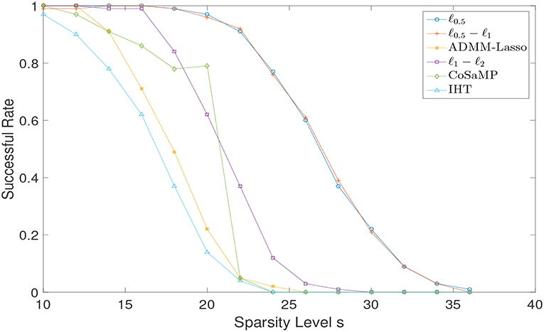
Figure 6. Sparse signal recovery performance comparison via different algorithms for Gaussian random matrix.
In this paper, we studied a new non-convex recovery method, developed as minimizing a weighted difference of ℓr (0 < r ≤ 1) norm and ℓ1 norm. We established the performance bounds for this problem based on both r-RIP and q-ratio CMSV. An algorithm was proposed to approximately solve the non-convex problem. Numerical experiments show that the proposed algorithm provides superior performance compared to the existing algorithms such as ADMM-Lasso, CoSaMP, IHT and ℓ1 − ℓ2 minimization.
Besides, there are some open problems left for future work. One is the convergence study of the proposed algorithm in section 3. Another one is the generalization of this 1-D non-convex version to 2-D non-convex total variation minimization as done in Lou et al. [39] and the exploration of its application to medical imaging. Moreover, analogous to the non-convex block-sparse compressive sensing studied in Wang et al. [40], the study of the following non-convex block-sparse recovery minimization problem:
where with z[i] denoting the i-th block of z, 0 ≤ α ≤ 1, and 0 < r ≤ 1, is also an interesting topic for further investigation.
ZZ contributed to the initial idea and wrote the first draft. JY provided critical feedback and helped to revise the manuscript.
This work is supported by the Swedish Research Council grant (Reg.No. 340-2013-5342).
The authors declare that the research was conducted in the absence of any commercial or financial relationships that could be construed as a potential conflict of interest.
1. ^ All figures can be reproduced from the code available at https://github.com/zzy583661/Weighted-l_r-l_1-minimization
1. Candes EJ, Tao T. Decoding by linear programming. IEEE Trans Inf Theory. (2005) 51:4203–15. doi: 10.1109/TIT.2005.858979
2. Donoho DL. Compressed sensing. IEEE Trans Inf Theory. (2006) 52:1289–306. doi: 10.1109/TIT.2006.871582
3. Eldar YC, Kutyniok G. Compressed Sensing: Theory and Applications. Cambridge: Cambridge University Press (2012).
4. Foucart S, Rauhut H. A Mathematical Introduction to Compressive Sensing. Vol. 1. New York, NY: Birkhäuser (2013).
5. Gribonval R, Nielsen M. Sparse representations in unions of bases. IEEE Trans Inf Theory. (2003) 49:3320–5. doi: 10.1109/TIT.2003.820031
6. Tropp JA. Greed is good: algorithmic results for sparse approximation. IEEE Trans Inf Theory. (2004) 50:2231–42. doi: 10.1109/TIT.2004.834793
7. Candes EJ. The restricted isometry property and its implications for compressed sensing. Comptes Rendus Math. (2008) 346:589–92. doi: 10.1016/j.crma.2008.03.014
8. Candes EJ, Romberg JK, Tao T. Stable signal recovery from incomplete and inaccurate measurements. Commun Pure Appl Math. (2006) 59:1207–23. doi: 10.1002/cpa.20124
9. Cohen A, Dahmen W, DeVore R. Compressed sensing and best k-term approximation. J Am Math Soc. (2009) 22:211–31. doi: 10.1090/S0894-0347-08-00610-3
10. Dirksen S, Lecué G, Rauhut H. On the gap between restricted isometry properties and sparse recovery conditions. IEEE Trans Inf Theory. (2018) 64:5478–87. doi: 10.1109/TIT.2016.2570244
11. Tang G, Nehorai A. Performance analysis of sparse recovery based on constrained minimal singular values. IEEE Trans Signal Process. (2011) 59:5734–45. doi: 10.1109/TSP.2011.2164913
12. Zhou Z, Yu J. Sparse recovery based on q-ratio constrained minimal singular values. Signal Process. (2019) 155:247–58. doi: 10.1016/j.sigpro.2018.10.002
13. Chen SS, Donoho DL, Saunders MA. Atomic decomposition by basis pursuit. SIAM J Sci Comput. (1998) 20:33–61.
14. Natarajan BK. Sparse approximate solutions to linear systems. SIAM J Sci Comput. (1995) 24:227–34. doi: 10.1137/S0097539792240406
15. Chartrand R. Exact reconstruction of sparse signals via nonconvex minimization. IEEE Signal Process Lett. (2007) 14:707–10. doi: 10.1109/LSP.2007.898300
16. Foucart S, Lai MJ. Sparsest solutions of underdetermined linear systems via ℓq-minimization for 0 < q ≤ 1. Appl Comput Harmon Anal. (2009) 26:395–407. doi: 10.1016/j.acha.2008.09.001
17. Li S, Lin J. Compressed Sensing with coherent tight frames via lq-minimization for 0 < q ≤ 1. Inverse Probl Imaging. (2014) 8:761–77. doi: 10.3934/ipi.2014.8.761
18. Lin J, Li S. Restricted q-isometry properties adapted to frames for nonconvex lq-analysis. IEEE Trans Inf Theory. (2016) 62:4733–47. doi: 10.1109/TIT.2016.2573312
19. Shen Y, Li S. Restricted p–isometry property and its application for nonconvex compressive sensing. Adv Comput Math. (2012) 37:441–52. doi: 10.1007/s10444-011-9219-y
20. Xu Z, Chang X, Xu F, Zhang H. L1/2 regularization: a thresholding representation theory and a fast solver. IEEE Trans Neural Netw Learn Syst. (2012) 23:1013–27. doi: 10.1109/TNNLS.2012.2197412
21. Chartrand R, Yin W. Iteratively reweighted algorithms for compressive sensing. In: IEEE International Conference on Acoustics, Speech and Signal Processing, 2008. (2008). p. 3869–72.
22. Lai MJ, Xu Y, Yin W. Improved iteratively reweighted least squares for unconstrained smoothed ℓq minimization. SIAM J Numer Anal. (2013) 51:927–57. doi: 10.1137/110840364
23. Lou Y, Yin P, He Q, Xin J. Computing sparse representation in a highly coherent dictionary based on difference of L1 and L2. J Sci Comput. (2015) 64:178–96. doi: 10.1007/s10915-014-9930-1
24. Yin P, Lou Y, He Q, Xin J. Minimization of ℓ1−2 for compressed sensing. SIAM J Sci Comput. (2015) 37:A536–63. doi: 10.1137/140952363
25. Yin P, Esser E, Xin J. Ratio and difference of l1 and l2 norms and sparse representation with coherent dictionaries. Commun Inf Syst. (2014) 14:87–109. doi: 10.4310/CIS.2014.v14.n2.a2
26. Lou Y, Yan M. Fast L1–L2 minimization via a proximal operator. J Sci Comput. (2018) 74:767–85. doi: 10.1007/s10915-017-0463-2
27. Wang Y. New Improved Penalty Methods for Sparse Reconstruction Based on Difference of Two Norms. Optimization Online, the Mathematical Optimization Society (2015). Available online at: http://www.optimization-online.org/DB_HTML/2015/03/4849.html
28. Wang D, Zhang Z. Generalized sparse recovery model and its neural dynamical optimization method for compressed sensing. Circ Syst Signal Process. (2017) 36:4326–53. doi: 10.1007/s00034-017-0532-7
29. Zhao Y, He X, Huang T, Huang J. Smoothing inertial projection neural network for minimization Lp−q in sparse signal reconstruction. Neural Netw. (2018) 99:31–41. doi: 10.1016/j.neunet.2017.12.008
30. Chartrand R, Staneva V. Restricted isometry properties and nonconvex compressive sensing. Inverse Probl. (2008) 24:035020. doi: 10.1088/0266-5611/24/3/035020
31. Lopes ME. Unknown sparsity in compressed sensing: denoising and inference. IEEE Trans Inf Theory. (2016) 62:5145–66. doi: 10.1109/TIT.2016.2587772
32. Zhou Z, Yu J. On q-ratio CMSV for sparse recovery. arXiv [Preprint]. arXiv:180512022. (2018). Available online at: https://arxiv.org/abs/1805.12022
33. Tran H, Webster C. Unified sufficient conditions for uniform recovery of sparse signals via nonconvex minimizations. arXiv preprint arXiv:171007348. (2017).
34. Tao PD, An LTH. Convex analysis approach to dc programming: theory, algorithms and applications. Acta Math Vietnam. (1997) 22:289–355.
35. Tao PD, An LTH. A DC optimization algorithm for solving the trust-region subproblem. SIAM J Optim. (1998) 8:476–505. doi: 10.1137/S1052623494274313
36. Boyd S, Parikh N, Chu E, Peleato B, Eckstein J, et al. Distributed optimization and statistical learning via the alternating direction method of multipliers. Found Trends Mach Learn. (2011) 3:1–122. doi: 10.1561/2200000016
37. Needell D, Tropp JA. CoSaMP: iterative signal recovery from incomplete and inaccurate samples. Appl Comput Harmon Anal. (2009) 26:301–21. doi: 10.1016/j.acha.2008.07.002
38. Blumensath T, Davies ME. Iterative hard thresholding for compressed sensing. Appl Comput Harmon Anal. (2009) 27:265–74. doi: 10.1016/j.acha.2009.04.002
39. Lou Y, Zeng T, Osher S, Xin J. A weighted difference of anisotropic and isotropic total variation model for image processing. SIAM J Imaging Sci. (2015) 8:1798–23. doi: 10.1137/14098435X
Keywords: compressive sensing, nonconvex sparse recovery, iteratively reweighted least squares, difference of convex functions, q-ratio constrained minimal singular values
Citation: Zhou Z and Yu J (2019) A New Nonconvex Sparse Recovery Method for Compressive Sensing. Front. Appl. Math. Stat. 5:14. doi: 10.3389/fams.2019.00014
Received: 28 September 2018; Accepted: 22 February 2019;
Published: 14 March 2019.
Edited by:
Jean-Luc Bouchot, Beijing Institute of Technology, ChinaReviewed by:
Junhong Lin, École Polytechnique Fédérale de Lausanne, SwitzerlandCopyright © 2019 Zhou and Yu. This is an open-access article distributed under the terms of the Creative Commons Attribution License (CC BY). The use, distribution or reproduction in other forums is permitted, provided the original author(s) and the copyright owner(s) are credited and that the original publication in this journal is cited, in accordance with accepted academic practice. No use, distribution or reproduction is permitted which does not comply with these terms.
*Correspondence: Zhiyong Zhou, emhpeW9uZy56aG91QHVtdS5zZQ==
Disclaimer: All claims expressed in this article are solely those of the authors and do not necessarily represent those of their affiliated organizations, or those of the publisher, the editors and the reviewers. Any product that may be evaluated in this article or claim that may be made by its manufacturer is not guaranteed or endorsed by the publisher.
Research integrity at Frontiers
Learn more about the work of our research integrity team to safeguard the quality of each article we publish.