On the Complexity of Sparse Label Propagation

This paper investigates the computational complexity of sparse label propagation which has been proposed recently for processing network-structured data. Sparse label propagation amounts to a convex optimization problem and might be considered as an extension of basis pursuit from sparse vectors to clustered graph signals representing the label information contained in network-structured datasets. Using a standard first-order oracle model, we characterize the number of iterations for sparse label propagation to achieve a prescribed accuracy. In particular, we derive an upper bound on the number of iterations required to achieve a certain accuracy and show that this upper bound is sharp for datasets having a chain structure (e.g., time series).

1. Introduction

A powerful approach to processing massive datasets is via using graph models. In particular, we consider datasets which can be characterized by an “empirical graph” (cf. [1, Ch. 11]) whose nodes represent individual data points and whose edges connect data points which are similar in an application-specific sense. The empirical graph for a particular dataset might be obtained by (domain) expert knowledge, an intrinsic network structure (e.g., for social network data) or in a data-driven fashion by imposing smoothness constrains on observed realizations of graph signals (which serve as training data) [2–8]. Besides the graph structure, datasets carry additional information in the form of labels (e.g., class membership) associated with individual data points. We will represent such label information as graph signals defined over the empirical graph [9].

Using graph signals for representing datasets is appealing for several reasons. Indeed, having a graph model for datasets facilitates scalable distributed data processing in the form of message passing over the empirical graph [10]. Moreover, graph models allow to cope with heterogeneous datasets containing mixtures of different data types, since they only require an abstract notion of similarity between individual data points. In particular, the structure encoded in the graph model of a dataset enables to capitalize, by exploiting the similarity between data points, on massive amounts of unlabeled data via semi-supervised learning [1]. This is important, since labeling of data points is often expensive and therefore label information is typically available only for a small fraction of the overall dataset. The labels of individual data points induce a graph signal which is defined over the associated empirical graph. We typically only have access to the signal values (labels) of few data points and the goal is learn or recover the remaining graph signal values (labels) for all other data points.

The processing of graph signals relies on particular models for graph signals. A prominent line of uses applies spectral graph theory to extend the notion of band-limited signals from the time domain (which corresponds to the special case of a chain graph) to arbitrary graphs [1, 9, 11–14]. These band-limited graph signals are smooth in the sense of having a small variation over well-connected subsets of nodes, where the variation is measured by the Laplacian quadratic form. However, our approach targets datasets whose labels induce piece-wise constant graph signals, i.e., the signal values (labels) of data points belonging to well connected subset of data points (clusters) [15], are nearly identical. This signal model is useful, e.g., in change-point detection, image segmentation or anomaly detection where signal values might change abruptly [16–20].

The closest to our work is Hallac et al.[16], Sharpnack et al. [17], and Wang et al.[18] for general graph models, as well as a line of work on total variation-based image processing [21–23]. In contrast to Chambolle [21], Chambolle and Pock [22], and Pock and Chambolle. [23], which consider only regular grid graphs, our approach applies to arbitrary graph topology. The methods presented in Fan and Guan [16], Sharpnack et al. [17], and Wang et al. [20] apply also to arbitrary graph topologies but require (noisy) labels available for all data points, while we consider labels available only on a small subset of nodes.

1.1. Contributions and Outline

In section 2, we formulate the problem of recovering clustered graph signals as a convex optimization problem. We solve this optimization problem by applying a preconditioned variant of the primal-dual method of Pock and Chambolle [23]. As detailed in section 3, the resulting algorithm can be implemented as a highly scalable message passing protocol, which we coin sparse label propagation (SLP). In section 4, we present our main result which is an upper bound on the number of SLP iterations ensuring a particular accuracy. We also discuss the tightness of the upper bound for datasets whose empirical graph is a chain graph (e.g, time series).

1.2. Notation

Given a vector $\mathbf{\text{x}}={(x_1,\dots ,x_n)}^T\in {ℝ}^n$, we define the norms $\left|\right|\mathbf{\text{x}}|{|}_1:=\sum _{l=1}^n|x_l|$ and $\left|\right|\mathbf{\text{x}}|{|}_2:=\sqrt{\sum _{l=1}^n{(x_l)}^2}$, respectively. The spectral norm of a matrix D is denoted $\left|\right|\mathbf{\text{D}}|{|}_2:={sup}_{\left|\right|\mathbf{\text{x}}|{|}_2=1}|\left|\mathbf{\text{D}}\mathbf{\text{x}}\right|{|}_2$. For a positive semidefinite (psd) matrix Q ∈ ℝ^n×n, with spectral decomposition $\text{Q}=\text{U}\text{diag}{\left\{q_i\right\}}_{i=1}^n{\text{U}}^T$, we define its square root as ${\text{Q}}^{1/2}:=\text{U}\text{diag}{\left\{\sqrt{q_i}\right\}}_{i=1}^n{\text{U}}^T$. For a positive definite matrix Q, we define the norm $\left|\right|\mathbf{\text{x}}|{|}_{\text{Q}}:=\sqrt{{\mathbf{\text{x}}}^T\text{Q}\mathbf{\text{x}}}$. The signum sign{x} of a vector x = (x₁, …, x_d) is defined as the vector $\left(\text{sign}(x_1),\dots ,\text{sign}(x_d)\in {ℝ}^d\right)$ with the scalar signum function

$\begin{array}{ll}\text{sign}(x_i)=\{\begin{array}{ll}-1\hfill & \text{ for }{x}_i<0\hfill \\ 0\hfill & \text{ for }{x}_i=0\hfill \\ 1\hfill & \text{ for }{x}_i>0.\hfill \end{array}& (1)\end{array}$

Throughout this paper we consider convex functions g(x) whose epigraphs epi g: = {(x, t):x ∈ ℝⁿ, g(x) ≤ t} ⊆ ℝⁿ×ℝ are non-empty closed convex sets [24]. Given such a convex function g(x), we denote its subdifferential at ${\mathbf{\text{x}}}_0\in {ℝ}^n$ by

$\begin{array}{l}\partial g({\text{x}}_0):=\left\{\text{y}\in {ℝ}^n:g(\text{x})\ge g({\text{x}}_0)+{\text{y}}^T(\text{x}-{\text{x}}_0)\mathrm{\text{for any }}\text{x}\right\}\subseteq {ℝ}^n\end{array}$

and its convex conjugate function by Boyd and Vandenberghe [25]

$\begin{array}{ll}{g}^{*}(\widehat{\text{y}}):={\displaystyle \underset{\text{y}\in {ℝ}^n}{sup}}{\text{y}}^T\widehat{\text{y}}-g(\text{y}).& (2)\end{array}$

We can re-obtain a convex function g(y) from its convex conjugate via [25]

$\begin{array}{ll}g(\widehat{\text{y}}):={\displaystyle \underset{\text{y}\in {ℝ}^n}{sup}}{\text{y}}^T\widehat{\text{y}}-g^{*}(\text{y}).& (3)\end{array}$

2. Problem Setting

We consider network-structured datasets which are represented by an undirected weighted graph ${G}=({V},{E},\text{W})$, referred to as the “empirical graph” (see Figure 1). The nodes $i\in {V}$ of the empirical graph represent individual data points, such as user profiles in a social network or documents of a repository. An undirected edge $\left\{i,j\right\}\in {E}$ of the empirical graph encodes a notion of (physical or statistical) proximity of neighboring data points, such as profiles of befriended social network users or documents which have been co-authored by the same person. This network structure is identified with conditional independence relations within probabilistic graphical models (PGM) [4–8].

FIGURE 1

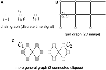
Figure 1. Some examples of network-structured datasets with associated empirical graph being (A) a chain graph (discrete time signals), (B) grid graph (2D-images) and (C) a clustered graph (social networks).

As opposed to PGM, we consider a fully deterministic graph-based model which does not invoke an underlying probability distribution for the observed data. In particular, given an edge $\left\{i,j\right\}\in {E}$, the nonzero value W_i,j > 0 represents the amount of similarity between the data points $i,j\in {V}$. The edge set ${E}$ can be read off from the non-zero pattern of the weight matrix W ∈ ℝ^N×N since

$\begin{array}{ll}\left\{i,j\right\}\in {E}\mathrm{\text{ if and only if }}{W}_{i,j}>0.& (4)\end{array}$

According to (4), we could in principle handle network-structured datasets using traditional multivariate (vector/matrix based) methods. However, putting the emphasis on the empirical graph leads naturally to scalable algorithms which are implemented as message passing methods (see Algorithm 2 below).

The neighborhood ${N}(i)$ and weighted degree (strength) d_i of node $i\in {V}$ are

$\begin{array}{ll}{N}(i):=\left\{j\in {V}:\left\{i,j\right\}\in {E}\right\}\mathrm{\text{, and }}{d}_i:={\displaystyle \sum _{j\in {N}(i)}}{W}_{i,j}\mathrm{\text{, respectively.}}& (5)\end{array}$

In what follows we assume the empirical graph to be connected, i.e., d_i > 0 for all nodes $i\in {V}$ and having no self-loops such that W_i,i = 0 for all $i\in {V}$. The maximum (weighted) node degree is

$\begin{array}{ll}{d}_{\text{max}}:=\underset{{}_{i\in \mathcal{V}}}{\max }{d}_i\stackrel{(5)}{=}\underset{i\in \mathcal{V}}{\max }{\displaystyle \sum _{j\in \mathcal{N}(i)}{W}_{i,j}}.& (6)\end{array}$

It will be convenient to orient the undirected empirical graph ${G}=({V},{E},\text{W})$, which yields the directed version $\vec{{G}}=({V},\vec{{E}},\mathbf{\text{W}})$. The orientation amounts to declaring for each edge e = {i, j} one node as the head (origin node) and the other node as the tail (destination node) denoted e⁺ and e⁻, respectively. Given a set of edges ${S}\subseteq {E}$ in the undirected graph ${G}$, we denote the corresponding set of directed edges in $\vec{{G}}$ as $\vec{{S}}$. The incidence matrix $\mathbf{\text{D}}\in {ℝ}^{\left|{E}\right|\times \left|{V}\right|}$ of $\vec{{G}}$ is [16]

$\begin{array}{ll}{D}_{e,i}=\{\begin{array}{ll}{W}_e\hfill & \text{if} i=e^{+}\hfill \\ -W_e\hfill & \text{if} i=e^{-}\hfill \\ 0\hfill & \text{else}.\hfill \end{array}& (7)\end{array}$

If we number the nodes and orient the edges in the chain graph in Figure 1A from left to right, its weighted incidence matrix would be

$\begin{array}{l}D=\left(\begin{array}{ccc}{W}_{1,2}& -W_{1,2}& 0\\ 0& W_{2,3}& -W_{2,3}\end{array}\right).\end{array}$

The directed neighborhoods of a node $i\in {V}$ are defined as ${{N}}_{+}(i):=\left\{j\in {V}:e=\left\{i,j\right\}\in {E}\mathrm{\text{, and, }}{e}^{+}=i\right\}$ and ${{N}}_{-}(i):=\left\{j\in {V}:e=\left\{i,j\right\}\in {E}\mathrm{\text{, and, }}{e}^{-}=i\right\}$, respectively. We highlight that the particular choice of orientation for the empirical graph ${G}$ has no effect on our results andmethods and will be only used for notational convenience.

In many applications we can associate each data point $i\in {V}$ with a label x_i, e.g., in a social network application the label x_i might encode the group membership of the member $i\in {V}$ in a social network ${G}$. We interpret the labels x_i as values of a graph signal x defined over the empirical graph ${G}$. Formally, a graph signal $\mathbf{\text{x}}\in {ℝ}^{{V}}$ defined over the graph ${G}$ maps each node $i\in {V}$ to the graph signal value x[i] ∈ ℝ. Since acquiring labels is often costly and error-prone, we typically have access to a few noisy labels ${\tilde{x}}_i$ for the data points $i\in {M}\subseteq {V}$ within a (small) subset ${M}\subseteq {V}$ of nodes in the empirical graph. Thus, we are interested in recovering the entire graph signal x from knowledge of its values $x\left[i\right]={\tilde{x}}_i$ on a small subset ${M}\subseteq {V}$ of labeled nodes $i\in {M}$. The signal recovery will be based on a clustering assumption [1]. Clustering Assumption (informal). Consider a graph signal $\mathbf{\text{x}}\in {ℝ}^{\left|{V}\right|}$ whose signal values are the (mostly unknown) labels ${\tilde{x}}_i$ of the data points $z_i\in {D}$. The signal values x[i], x[j] at nodes $i,j\in {V}$ within a well-connected subset (cluster) of nodes in the empirical graph are similar, i.e., x[i] ≈ x[j].

This assumption of clustered graph signals x can be made precise by requiring a small total variation (TV)

$\begin{array}{ll}\left|\right|\text{x}|{|}_{\text{TV}}:={\displaystyle \sum _{\left\{i,j\right\}\in {E}}}{W}_{i,j}|x\left[j\right]-x\left[i\right]|.& (8)\end{array}$

The incidence matrix D (cf. (7)) allows to represent the TV of a graph signal conveniently as

$\begin{array}{ll}\left|\right|\text{x}|{|}_{\text{TV}}=|\left|\text{D}\text{x}\right|{|}_1.& (9)\end{array}$

We note that related but different measures for the total variation of a graph signal have been proposed previously (see, e.g., [26, 27]). The definition (8) is appealing for several reasons. First, it conforms with the class of piece-wise constant or clustered graph signals which has proven useful in several applications including meteorology and binary classification [29, 28]. Second, as we demonstrate in what follows, the definition (8) allows to derive semi-supervised learning methods which can be implemented by efficient massing passing over the underlying empirical graph and thus ensure scalability of the resulting algorithm to large-scale (big) data.

A sensible strategy for recovering a graph signal with small TV is via minimizing the TV $\left|\right|\widetilde{\mathbf{\text{x}}}|{|}_{\text{TV}}$ while requiring consistency with the observed noisy labels ${\left\{{\tilde{x}}_i\right\}}_{i\in {M}}$, i.e.,

$\begin{array}{l}{\widehat{\mathbf{x}}}_{\text{SLP}}\in \underset{x\in {ℝ}^{\left|\mathcal{V}\right|}}{\arg \min }{\displaystyle \sum _{\{i,j\}\in \mathcal{E}}{W}_{i,j}}|x[j]\text{}-\text{}x[i]|\text{s}\text{.t}\text{.}x[i]\text{}=\text{}{\tilde{x}}_i\text{ for all }i\in \mathcal{M}\\ \stackrel{(9)}{=}\underset{x\in {ℝ}^{\left|\mathcal{V}\right|}}{\arg \min }\Vert \mathbf{D}\mathbf{x}{\Vert }_1\text{s}\text{.t}\text{.}x[i]\text{}=\text{}{\tilde{x}}_i\text{ for all }i\in \mathcal{M}.& (10)\end{array}$

The objective function of the optimization problem (10) is the seminorm ||x||_TV, which is a convex function. ¹ Since moreover the constraints in (10) are linear, the optimization problem (10) is a convex optimization problem [25]. Rather trivially, the problem (10) is equivalent to

$\begin{array}{ll}{\widehat{\text{x}}}_{\text{SLP}}={\displaystyle \underset{\text{x}\in {Q}}{\mathrm{\text{arg min}}}}\left|\right|\text{Dx}|{|}_1.& (11)\end{array}$

Here, we used the constraint set ${Q}=\left\{\mathbf{\text{x}}:x\left[i\right]={\tilde{x}}_i\mathrm{\text{ for all }}i\in {M}\right\}$ which collects all graph signals $\mathbf{\text{x}}\in {ℝ}^{\left|{V}\right|}$ which match the observed labels ${\tilde{x}}_i$ for the nodes of the sampling set ${M}$.

The usefulness of the learning problem (10) depends on two aspects: (i) the deviation of the solutions of (10) from the true underlying graph signal and (ii) the difficulty (complexity) of computing the solutions of (10). The first aspect has been addressed in [30] which presents precise conditions on the sampling set ${M}$ and topology of the empirical graph ${G}$ such that any solution of (10) is close to the true underlying graph signal if it is (approximately) piece-wise constant over well-connected subsets of nodes (clusters). The focus of this paper is the second aspect, i.e., the difficulty or complexity of computing approximate solutions of (10).

In what follows we will apply an efficient primal-dual method to solving the convex optimization problem (10). This primal-dual method is appealing since it provides a theoretical convergence guarantee and also allows for an efficient implementation as message passing over the underlying empirical graph (cf. Algorithm 2 below). We coin the resulting semi-supervised learning algorithm sparse label propagation (SLP) since it bears some conceptual similarity to the ordinary label propagation (LP) algorithm for semi-supervised learning over graph models. In particular, LP algorithms can be interpreted as message passing methods for solving a particular recovery (or, learning) problem [1, Chap 11.3.4.]:

$\begin{array}{ll}{\widehat{\text{x}}}_{\text{LP}}\in {\displaystyle \underset{\text{x}\in {ℝ}^{\left|{V}\right|}}{\mathrm{\text{arg min}}}}{\displaystyle \sum _{\left\{i,j\right\}\in {E}}}{W}_{i,j}{(x\left[i\right]-x\left[j\right])}^2\mathrm{\text{s}}.\text{t}.x\left[i\right]={\tilde{x}}_i\mathrm{\text{for all }}i\in {M}.& (12)\end{array}$

The recovery problem (12) amounts to minimizing the weighted sum of squares, while SLP (10) minimize a weighted sum of absolute values, of the signal differences (x[i] − x[j])² arising over the edges $\left\{i,j\right\}\in {E}$ in the empirical graph ${G}$. It turns out that using the absolute values of signal differences instead of their squares allows SLP methods to accurately learn graph signals x which vary abruptly over few edges, e.g., clustered graph signals considered in [29, 28]. In contrast, LP methods tends to smooth out such abrupt signal variations.

The SLP problem (10) is also closely related to the recently proposed network Lasso [18, 31]

$\begin{array}{ll}{\widehat{\text{x}}}_{\text{nLasso}}\in {\displaystyle \underset{\text{x}\in {ℝ}^{\left|{V}\right|}}{\mathrm{\text{arg min}}}}{\displaystyle \sum _{i\in {M}}}{(x\left[i\right]-{\tilde{x}}_i)}^2+\lambda \left|\right|\text{x}|{|}_{\text{TV}}.& (13)\end{array}$

Indeed, according to Lagrangian duality [32, 25], by choosing λ in (13) suitably, the solutions of (13) coincide with those of (10). The tuning parameter λ trades small empirical label fitting error $\sum _{i\in {M}}{(x\left[i\right]-{\tilde{x}}_i)}^2$ against small total variation $\left|\right|{\widehat{\mathbf{\text{x}}}}_{\text{nLasso}}|{|}_{\text{TV}}$ of the learned graph signal ${\widehat{\mathbf{\text{x}}}}_{\text{nLasso}}$. Choosing a large value of λ enforces small total variation of the learned graph signal, while using a small value for λ puts more emphasis on the empirical error. In contrast to network Lasso (13), which requires to choose the parameter λ (e.g., using (cross-)validation [33, 34]), the SLP method (10) does not require any parameter tuning.

3. Sparse Label Propagation

The recovery problem (10) is a convex optimization problem with a non-differentiable objective function, which precludes the use of standard gradient methods such as (accelerated) gradient descent. However, both the objective function and the constraint set of the optimization problem (10) have rather a simple structure individually. This suggests the use of efficient proximal methods [35] for solving (10). In particular, we apply a preconditioned variant of the primal-dual method introduced by [36] to solve (10).

In order to apply the primal-dual method of [36], we reformulate (10) as an unconstrained problem (see (11))

$\begin{array}{l}{\widehat{\text{x}}}_{\text{SLP}}\in {\displaystyle \underset{\text{x}\in {ℝ}^{\left|{V}\right|}}{\mathrm{\text{arg min}}}}f(\text{x}):=g(\text{D}\text{x})+h(\text{x}),\mathrm{\text{with }}g(\text{y})\\ :=\left|\right|\text{y}|{|}_1\mathrm{\text{and }}h(\text{x}):=\{\begin{array}{c}\infty \mathrm{\text{ if }}\text{x} \notin {Q}\hfill \\ 0\mathrm{\text{ if }}\text{x} \in {Q}.\hfill \end{array}& (14)\end{array}$

The function h(x) in (14) is the indicator function (cf. [24]) of the convex set ${Q}$ and can be described also via its epigraph

$\begin{array}{l}\text{epi }h=\left\{(\text{x},t):\text{x}\in {Q},t\ge 0\right\}\subseteq {ℝ}^{\left|{V}\right|}\times ℝ.\end{array}$

It will be useful to define another optimisation problem which might be considered as a dual problem to (14), i.e.,

$\begin{array}{ll}{\widehat{\text{y}}}_{\text{SLP}}\in {\displaystyle \underset{\text{y}\in {ℝ}^{\left|{E}\right|}}{\mathrm{\text{arg max}}}}\tilde{f}(\text{y}):=-h^{*}(-{\text{D}}^T\text{y})-g^{*}(\text{y}).& (15)\end{array}$

Note that the objective function $\tilde{f}(\mathbf{\text{y}})$ of the dual SLP problem (15) involves the convex conjugates h*(x) and g*(y) (cf. (2)) of the convex functions h(x) and g(y) which define the primal SLP problem (14).

By elementary convex analysis [24], the solutions ${\widehat{\mathbf{\text{x}}}}_{\text{SLP}}$ of (14) are characterized by the zero-subgradient condition

$\begin{array}{ll}0\in \partial f({\widehat{\text{x}}}_{\text{SLP}}).& (16)\end{array}$

A particular class of iterative methods for solving (14), referred to as proximal methods, is obtained via fixed-point iterations of some operator ${P}:{ℝ}^{\left|{V}\right|}\to {ℝ}^{\left|{V}\right|}$ whose fixed-points are precisely the solutions ${\widehat{\mathbf{\text{x}}}}_{\text{SLP}}$ of (16), i.e.,

$\begin{array}{ll}0\in \partial f({\widehat{\text{x}}}_{\text{SLP}})\mathrm{\text{ if and only if }}{\widehat{\text{x}}}_{\text{SLP}}={P}{\widehat{\text{x}}}_{\text{SLP}}.& (17)\end{array}$

In general, the operator ${P}$ is not unique, i.e., there are different choices for ${P}$ such that (17) is valid. These different choices for the operator ${P}$ in (17) result in different proximal methods [35].

One approach to constructing the operator ${P}$ in (17) is based on convex duality [24, Thm. 31.3], according to which a graph signal ${\widehat{\mathbf{\text{x}}}}_{\text{SLP}}\in {ℝ}^{\left|{V}\right|}$ solves (14) if and only if there exists a (dual) vector $\widehat{\mathbf{\text{y}}}\in {ℝ}^{\left|{E}\right|}$ such that

$\begin{array}{ll}-({\text{D}}^T{\widehat{\text{y}}}_{\text{SLP}})\in \partial h({\widehat{\text{x}}}_{\text{SLP}})\mathrm{\text{, and, }}\text{D}{\widehat{\text{x}}}_{\text{SLP}}\in \partial g^{*}({\widehat{\text{y}}}_{\text{SLP}}).& (18)\end{array}$

The dual vector ${\widehat{\mathbf{\text{y}}}}_{\text{SLP}}\in {ℝ}^{\left|{E}\right|}$ represents a signal defined over the edges ${E}$ in the empirical graph ${G}$, with the entry ŷ_SLP[e] being the signal value associated with the particular edge $e\in {E}$.

Let us now rewrite the two coupled conditions in (18) as

$\begin{array}{l}{\widehat{\text{x}}}_{\text{SLP}}-\Gamma {\text{D}}^T{\widehat{\text{y}}}_{\text{SLP}}\in {\widehat{\text{x}}}_{\text{SLP}}+\Gamma \partial h({\widehat{\text{x}}}_{\text{SLP}})\mathrm{\text{, and, }}2\Lambda \text{D}{\widehat{\text{x}}}_{\text{SLP}}+{\widehat{\text{y}}}_{\text{SLP}}\\ \in \Lambda \partial g^{*}({\widehat{\text{y}}}_{\text{SLP}})+\Lambda \text{D}{\widehat{\text{x}}}_{\text{SLP}}+{\widehat{\text{y}}}_{\text{SLP}},& (19)\end{array}$

with the invertible diagonal matrices (cf. (4) and (5))

$\begin{array}{l}\Lambda :=(1/2)\text{diag}{\left\{{\lambda }_{\left\{i,j\right\}}=1/W_{i,j}\right\}}_{\left\{i,j\right\}\in {E}}\in {ℝ}^{\left|{E}\right|\times \left|{E}\right|}\mathrm{\text{and }}\Gamma \\ :=(1/2)\text{diag}{\left\{{\gamma }_i=1/d_i\right\}}_{i\in {V}}\in {ℝ}^{\left|{V}\right|\times \left|{V}\right|}.& (20)\end{array}$

The specific choice (20) for the matrices Γ and Λ can be shown to satisfy [23, Lemma 2]

$\begin{array}{ll}\left|\right|{\Gamma }^{1/2}{\text{D}}^T{\Lambda }^{1/2}|{|}_2\le 1/2,& (21)\end{array}$

which will turn out to be crucial for ensuring the convergence of the iterative algorithm we will propose for solving (14).

It will be convenient to define the resolvent operator for the functions g*(y) and h(x) (cf. (14) and (2)), [23, section 1.1.]

$\begin{array}{l}{(\text{I}+\Lambda \partial g^{*})}^{-1}(\text{y}):={\displaystyle \underset{\text{z}\in {ℝ}^{\left|{E}\right|}}{\mathrm{\text{arg min }}}}{g}^{*}(\text{z})+(1/2){(\text{y}-\text{z})}^T{\Lambda }^{-1}(\text{y}-\text{z})\mathrm{\text{, and, }}\\ {(\text{I}+\Gamma \partial h)}^{-1}(\text{x}):={\displaystyle \underset{\text{z}\in {ℝ}^{\left|{V}\right|}}{\mathrm{\text{arg min }}}}h(\text{z})+(1/2){(\text{x}-\text{z})}^T{\Gamma }^{-1}(\text{x}-\text{z}).& (22)\end{array}$

We can now rewrite the optimality condition (3) (for ${\widehat{\mathbf{\text{x}}}}_{\text{SLP}}$, ${\widehat{\mathbf{\text{y}}}}_{\text{SLP}}$ to be primal and dual optimal) more compactly as

$\begin{array}{l}{\widehat{\text{x}}}_{\text{SLP}}={(\text{I}+\Gamma \partial h)}^{-1}({\widehat{\text{x}}}_{\text{SLP}}-\Gamma {\text{D}}^T{\widehat{\text{y}}}_{\text{SLP}})\\ {\widehat{\text{y}}}_{\text{SLP}}-2{(\text{I}+\Lambda \partial g^{*})}^{-1}\Lambda \text{D}{\widehat{\text{x}}}_{\text{SLP}}={(\text{I}+\Lambda \partial g^{*})}^{-1}({\widehat{\text{y}}}_{\text{SLP}}-\Lambda \text{D}{\widehat{\text{x}}}_{\text{SLP}}).& (23)\end{array}$

The characterization (23) of the solution ${\widehat{\mathbf{\text{x}}}}_{\text{SLP}}\in {ℝ}^{\left|{V}\right|}$ for the SLP problem (10) leads naturally to the following fixed-point iterations for finding ${\widehat{\mathbf{\text{x}}}}_{\text{SLP}}$ (cf.[23])

$\begin{array}{l}{\widehat{\text{y}}}^{(k+1)}:={(\text{I}+\Lambda \partial g^{*})}^{-1}({\widehat{\text{y}}}^{(k)}+\Lambda \text{D}(2{\widehat{\text{x}}}^{(k)}-{\widehat{\text{x}}}^{(k-1)}))\\ {\widehat{\text{x}}}^{(k+1)}:={(\text{I}+\Gamma \partial h)}^{-1}({\widehat{\text{x}}}^{(k)}-\Gamma {\text{D}}^T{\widehat{\text{y}}}^{(k+1)}).& (24)\end{array}$

The fixed-point iterations (24) are similar to those considered in [36, section 6.2.] for grid graphs arising in image processing. In contrast, the iterations (24) are formulated for an arbitrary graph (network) structure which is represented by the incidence matrix $\mathbf{\text{D}}\in {ℝ}^{\left|{E}\right|\times \left|{V}\right|}$. By evaluating the application of the resolvent operators (cf. (22)), we obtain simple closed-form expressions (cf. [36, section 6.2.]) for the updates in (24) yielding, in turn, Algorithm 1.

ALGORITHM 1

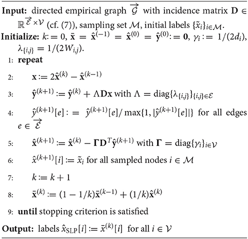
Algorithm 1. Sparse Label Propagation

Note that the Algorithm 1 does not directly output the iterate ${\widehat{\mathbf{\text{x}}}}^{(k)}$ but its running average ${\overline{\mathbf{\text{x}}}}^{(k)}$. Computing the running average (see step 8 in Algorithm 1) requires only little effort but allows for a simpler convergence analysis (see the proof of Theorem 1 in the Appendix).

One of the appealing properties of Algorithm 1 is that it allows for a highly scalable implementation via message passing over the underlying empirical graph ${G}$. This message passing implementation, summarized in Algorithm 1, is obtained by implementing the application of the graph incidence matrix D and its transpose D^T (cf. steps 2 and 5 of Algorithm 1) by local updates of the labels $\widehat{x}\left[i\right]$, i.e., updates which involve only the neighborhoods ${N}(i)$, ${N}(j)$ of all edges $\left\{i,j\right\}\in {E}$ in the empirical graph ${G}$.

Note that executing Algorithm 2 does not require to collect global knowledge about the entire empircal graph (such as the maximum node degree d_max (6)) at some central processing unit. Indeed, if we associate each node in the data graph with a computational unit, the execution of Algorithm 2 requires each node $i\in {V}$ only to store the values ${\left\{ŷ\left[\left\{i,j\right\}\right],W_{i,j}\right\}}_{j\in {N}(i)}$ and ${\widehat{x}}^{(k)}\left[i\right]$. Moreover, the number of arithmetic operations required at each node $i\in {V}$ during each time step is proportional to the number of the neighbors ${N}(i)$. These characteristics allow Algorithm 2 to scale to massive datasets (big data) if they can be represented using sparse networks having a small maximum degree d_max (6)). The datasets generated in many important applications have been found to be accurately represented by such sparse networks [37].

ALGORITHM 2

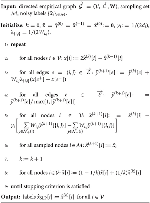
Algorithm 2. Sparse Label Propagation as Message Passing

4. Complexity of Sparse Label Propagation

There are various options for the stopping criterion in Algorithm 1, e.g., using a fixed number of iterations or testing for sufficient decrease of the objective function (cf.[38]). When using a fixed number of iterations, the following characterization of the convergence rate of Algorithm 1, we need to have a precise characterization of how many iterations are required to guarantee a prescribed accuracy of the resulting estimate. Such a characterization is provided by the following result.

Theorem 1. Consider the sequences ${\widehat{\mathbf{\text{x}}}}^{(k)}$ and ${\widehat{\mathbf{\text{y}}}}^{(k)}$ obtained from the update rule (24) and starting from some arbitrary initalizations ${\widehat{\mathbf{\text{x}}}}^{(0)}$ and ${\widehat{\mathbf{\text{y}}}}^{(0)}$. The averages

$\begin{array}{ll}{\bar{\text{x}}}^{(K)}=(1/K){\displaystyle \sum _{k=1}^K}{\widehat{\text{x}}}^{(k)}\mathrm{, and, }{\bar{\text{y}}}^{(K)}=(1/K){\displaystyle \sum _{k=1}^K}{\widehat{\text{y}}}^{(k)}& (25)\end{array}$

obtained after K iterations (for k = 0, …, K − 1) of (24), satisfy

$\begin{array}{ll}{\Vert {\overline{\mathbf{\text{x}}}}^{\left(K\right)}\Vert }_{\text{TV}}-{\Vert {\widehat{\mathbf{\text{x}}}}_{\text{SLP}}\Vert }_{\text{TV}}\le \frac{1}{2K}\left({\Vert {\widehat{\mathbf{\text{x}}}}^{\left(0\right)}-{\widehat{\mathbf{\text{x}}}}_{\text{SLP}}\Vert }_{{\Gamma }^{-1}}^2+{\Vert {\widehat{\mathbf{\text{y}}}}^{\left(0\right)}-{\widetilde{\mathbf{\text{y}}}}^{\left(K\right)}\Vert }_{{\Lambda }^{-1}}^2\right)& (26)\end{array}$

with ${\widetilde{\mathbf{\text{y}}}}^{(K)}=\text{sign}\left\{\mathbf{\text{D}}{\overline{\mathbf{\text{x}}}}^{(K)}\right\}$. Moreover, the sequence $\left|\right|{\widehat{\mathbf{\text{y}}}}^{(0)}-{\widetilde{\mathbf{\text{y}}}}^{(K)}|{|}_{{\Lambda }^{-1}}$, for K = 1, …, is bounded.

Proof. see Appendix.□

According to (26), the sub-optimality in terms of objective value function incurred by the output of Algorithm 1 after K iterations is bounded as

$\begin{array}{ll}\left|\right|{\bar{\text{x}}}^{(K)}|{|}_{\text{TV}}-|\left|{\widehat{\text{x}}}_{\text{SLP}}\right|{|}_{\text{TV}}\le c/K,& (27)\end{array}$

where the constant c does not depend on K but might depend on the empirical graph via its weighted incidence matrix D (cf. (7)) as well as on the initial labels ${\tilde{x}}_i$. The bound (27) suggests that in order to ensure reducing the sub-optimality by a factor of two, we need to run Algorithm 1 for twice as many iterations.

Let us now show that the bound (27) on the convergence speed is essentially tight. What is more, the bound cannot be improved substantially by any learning method, such as SLP (14) or network Lasso (13), which is implemented as message passing over the underlying empirical graph ${G}$. To this end we consider a dataset whose empirical graph is a weighted chain graph (see Figure 2) with nodes ${V}=\left\{1,\dots ,N\right\}$ which are connected by N − 1 edges ${E}={\left\{\left\{i,i+1\right\}\right\}}_{i=1,\dots ,N-1}$. The weights of the edges are W_i,i+1 = 1/i. The labels of the data points ${V}$ induce a graph signal x defined over ${G}$ with x[i] = 1 for all nodes i = {1, …, N − 1} and x[N] = 0. We observe the graph signal noise free on the sampling set ${M}=\left\{1,N\right\}$, resulting in the observations ${\tilde{x}}_1=1$ and ${\tilde{x}}_N=0$. According to [30, Theorem 3], the solution ${\widehat{\mathbf{\text{x}}}}_{\text{SLP}}$ of the SLP problem (14) is unique and coincides with the true underlying graph signal x. Thus, the optimal objective function value is $\left|\right|{\widehat{\mathbf{\text{x}}}}_{\text{SLP}}|{|}_{\text{TV}}=|\left|\mathbf{\text{x}}\right|{|}_{\text{TV}}=1/(N-1)$. On the other hand, the output ${\overline{\mathbf{\text{x}}}}^{(K)}$ of Algorithm 1 after K iterations satisfies ${\bar{x}}^{(K)}\left[1\right]=1$ and ${\bar{x}}^{(K)}\left[i\right]=0$ for all nodes i ∈ {K + 1, …, N}. Thus,

$\begin{array}{ll}\left|\right|{\bar{\text{x}}}^{(K)}|{|}_{\text{TV}}\ge 1/W_{K,K+1}=1/K,& (28)\end{array}$

implying, in turn,

$\begin{array}{ll}\left|\right|{\bar{\text{x}}}^{(K)}|{|}_{\text{TV}}-|\left|{\widehat{\text{x}}}_{\text{SLP}}\right|{|}_{\text{TV}}\ge 1/K-1/N.& (29)\end{array}$

FIGURE 2

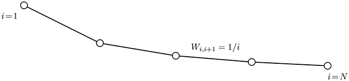
Figure 2. The empirical graph ${G}$ is a chain graph with edge weights W_i,i+1 = 1/i. We aim at recovering the graph a graph signal from the observations ${\tilde{x}}_1=1$ and ${\tilde{x}}_N=0$ using Algorithm 2.

For the regime of K/N ≪ 1 which is reasonable for big data applications where the number of iterations K computed in Algorithm 1 is small compared to the size N of the dataset, the dependency of the lower bound (29) on the number of iterations is essentially ∝1/K and therefore matches the upper bound (27). This example indicates that, for certain structure of edge weights, chain graphs are among the most challenging topologies regarding the convergence speed of SLP.

5. Conclusions

We have studied the intrinsic complexity of sparse label propagation by deriving an upper bound on the number of iterations required to achieve a given accuracy. This upper bound is essentially tight as it cannot be improved substantially for the particular class of graph signals defined over a chain graph (such as time series).

Author Contributions

The author confirms being the sole contributor of this work and approved it for publication.

Conflict of Interest Statement

The author declares that the research was conducted in the absence of any commercial or financial relationships that could be construed as a potential conflict of interest.

Supplementary Material

The Supplementary Material for this article can be found online at: https://www.frontiersin.org/articles/10.3389/fams.2018.00022/full#supplementary-material

Footnotes

1. ^The seminorm ||x||_TV is convex since it is homogeneous (||αx||_TV = |α|||x||_TV for α ∈ ℝ) and satisfies the triangle inequality (||x+y||_TV ≤ ||x||_TV+||y||_TV). These two properties imply convexity [25, section 3.1.5].

References

1. Chapelle O, Schölkopf B, Zien A. editors. Semi-Supervised Learning. Cambridge, Massachusetts: The MIT Press (2006).

Google Scholar

2. Zhu Z, Jin S, Song X, Luo X. Learning graph structure with stationary graph signals via first-order approximation. In: 2017 22nd International Conference on Digital Signal Processing (DSP), (London) (2017). 1–5.

Google Scholar

3. Kalofolias V. How to learn a graph from smooth signals. In: A. Gretton and C. C. Robert, editors, Proceedings of the 19th International Conference on Artificial Intelligence and Statistics, volume 51 of Proceedings of Machine Learning Research, (Cadiz) (2016). 920–9.

Google Scholar

4. Jung A. Learning the conditional independence structure of stationary time series: a multitask learning approach. IEEE Trans. Signal Process. (2015) 63:21. doi: 10.1109/TSP.2015.2460219

CrossRef Full Text | Google Scholar

5. Jung A, Hannak G, Görtz N. Graphical LASSO Based Model Selection for Time Series. IEEE Sig. Proc. Lett. (2015) 22:1781–5.

Google Scholar

6. Jung A, Heckel R, Bölcskei H, Hlawatsch F. Compressive nonparametric graphical model selection for time series. In: IEEE International Conference on Acoustics, Speech and Signal Processing (Florence) (2014).

Google Scholar

7. Quang NT, Jung A. Learning conditional independence structure for high-dimensional uncorrelated vector processes. In: IEEE International Conference on Acoustics, Speech and Signal Processing (ICASSP) (New Orleans, LA) (2017). 5920–5924.

Google Scholar

8. Quang NT, Jung A. On the sample complexity of graphical model selection from non-stationary samples. In: IEEE International Conference on Acoustics, Speech and Signal Processing (Calgary, AB) (2018).

9. Zhu X, Ghahramani Z. Learning From Labeled and Unlabeled Data With Label Propagation. Technical report, School of Computer Science Carnegie Mellon University (2002).

10. Sandryhaila A, Moura JMF. Big data analysis with signal processing on graphs: Representation and processing of massive data sets with irregular structure. IEEE Signal Process. Magaz. (2014) 31:80–90.

Google Scholar

11. Chen S, Sandryhaila A, Moura JMF, Kovačević J. Signal denoising on graphs via graph filtering. In: IEEE Global Conference on Signal and Information Processing (Atlanta, GA), (2014). 872–876.

Google Scholar

12. Chen S, Sandryhaila A, Kovačević J. Sampling theory for graph signals. In: IEEE International Conference on Acoustics, Speech and Signal Processing (Brisbane, QLD) (2015). 3392–6.

Google Scholar

13. Chen S, Varma R, Sandryhaila A, Kovačević J. Discrete signal processing on graphs: Sampling theory. IEEE Trans. Signal Process. (2015) 63:6510–23.

Google Scholar

14. Gadde A, Anis A, Ortega A. Active semi-supervised learning using sampling theory for graph signals. In: Proceedings of the 20th ACM SIGKDD International Conference on Knowledge Discovery and Data Mining (New York, NY) (2014). 492–501.

Google Scholar

15. Fortunato S. Community detection in graphs. (2009) arXiv.

Google Scholar

16. Sharpnack J, Rinaldo A, Singh A. Sparsistency of the edge lasso over graphs. AIStats (JMLR WCP) (La Palma) (2012).

Google Scholar

17. Wang Y-X, Sharpnack J, Smola AJ, Tibshirani RJ. Trend filtering on graphs. J. Mach. Lear. Res. (2016). 17:15–14.

Google Scholar

18. Hallac D, Leskovec J, Boyd S. Network lasso: clustering and optimization in large graphs. In: Proceedings SIGKDD (Sydney) (2015). 387–96.

PubMed Abstract | Google Scholar

19. Chen S, Varma R, Singh A, Kovačević J. Representations of piecewise smooth signals on graphs. In: Proc. IEEE ICASSP 2016, pages, March 2016.

20. Fan Z, Guan L. Approximate l0-penalized estimation of piecewise-constant signals on graphs. (2017) arxiv.

21. Chambolle A. An algorithm for total variation minimization and applications. J. Math. Imaging Vis. (2004) 20:89–97. doi: 10.1023/B:JMIV.0000011325.36760.1e

CrossRef Full Text | Google Scholar

22. Chambolle V, Pock T. An introduction to continuous optimization for imaging. Acta Numer. (2016) 25:161–319. doi: 10.1017/S096249291600009X

CrossRef Full Text | Google Scholar

23. Pock T. Chambolle A. Diagonal preconditioning for first order primal-dual algorithms in convex optimization. In: IEEE International Conference on Computer Vision (ICCV), (Barcelona) (2011).

24. Rockafellar RT. Convex Analysis. Princeton, NJ: Princeton University Press (1970).

Google Scholar

25. Boyd S, Vandenberghe L. Convex Optimization. Cambridge, UK: Cambridge University Press (2004).

Google Scholar

26. Chen S, Sandryhaila A, Moura JMF, Kovačević J. Signal recovery on graphs: Variation minimization. IEEE Trans Signal Process. (2015) 63:4609–24. doi: 10.1109/TSP.2015.2441042

CrossRef Full Text | Google Scholar

27. Sandryhaila A, Moura JMF. Discrete signal processing on graphs. IEEE Trans. Signal Process. (2013) 61:1644–56.

Google Scholar

28. Chen S, Varma R, Sandryhaila A, Kovačević J. Representations of piecewise smooth signals on graphs. In: 2016 IEEE International Conference on Acoustics, Speech and Signal Processing (Shanghai) (2016). 6370–74.

Google Scholar

29. Ambos AJH, Tran N. The logistic network lasso. (2018) arXiv.

Google Scholar

30. Jung A, Hulsebos M. The network nullspace property for compressed sensing of big data over networks. (2018) Front. Appl. Math. Stat. 4:9. doi: 10.3389/fams.2018.00009

CrossRef Full Text | Google Scholar

31. Jung A, Quang N, Mara A. When is network lasso accurate? (2018) Front. Appl. Math. Stat. 3:28.

Google Scholar

32. Bertsekas DP. Nonlinear Programming. Belmont, MA: Athena Scientific (2016).

Google Scholar

33. Jung A. A Gentle Introduction to Supervised Machine Learning. (2018) arXiv.

Google Scholar

34. Hastie T, Tibshirani R, Friedman J. The Elements of Statistical Learning. Springer; New York, NY: Springer Series in Statistics (2001).

Google Scholar

35. Parikh N. Boyd S. Proximal algorithms. Found Trends Optimizat. (2013) 1:123–231.

Google Scholar

36. Chambolle A, Pock T. A first-order primal-dual algorithm for convex problems with applications to imaging. J Math Imaging Vi. (2011) 40:120–145. doi: 10.1007/s10851-010-0251-1

CrossRef Full Text | Google Scholar

37. Barabási AL, Pósfai M. Network Science. Cambridge, UK: Cambridge University Press (2016).

Google Scholar

38. Becker S, Bobin J, Candès EJ. NESTA: a fast and accurate first-order method for sparse recovery. SIAM J Imaging Sci. (2011) 4:1–39. doi: 10.1137/090756855

CrossRef Full Text | Google Scholar