Mean-ETL Optimization in HorseRace Competition

In this paper, we present the methodology and results of the portfolios submitted to the HorseRace competition. The nine portfolios were constructed by applying the Mean-ETL optimization approach. The Mean-ETL optimization approach uses three fundamental variables (CTEF, MQ, and REG10) and three stock universes (GL, XUS, and EM), with each of the three fundamental variables applied one at a time to one of the three universes. This study assesses the return of the nine portfolios, and we report that all of these Mean-ETL portfolios produce positive active returns and most of them are statistically significant. Additionally, MQ variable is found to be the best among these three variables in the Mean-ETL portfolio construction.

1. Introduction

Fundamental data of stock markets have been researched and used in stock selection, portfolio construction for a long time. As an addition to the CAPM model for the stock market, Fama, and French [1] proposed the three famous factors: market factor, size factor, and value factor. Since Fama and French's finding in 1993, there have been many researches on portfolio construction with these fundamental variables. Jegadeesh and Titman [2] show that price momentum effect can generate statistically significant positive returns over certain holding periods. Guerard et al. [3] developed the United States Expected Returns (USER) stock selection model with ten fundamental variables, which will be described in greater details in the later section.

Modem Portfolio Theory (MPT) started with Markowitz's pioneering work [4] in 1952, which established the mean-variance portfolio optimization framework that maximizes the expected return for a given level of risk. Guerard and Takano [5] reported mean-variance portfolios with a composite model of the fundamental variables in the U.S. and Japanese stock markets outperformed their benchmarks by approximately 4% annually. After 25 years since the 1992 finding, Guerard [6] reported that the original model in Guerard and Takano [5] continued to be effective, which is a remarkable out-of-sample test of the original stock selection model.

Mean-ETL portfolio construction on the fundamental variables has been investigated in the past, e.g., Guerard [7] studied the Global Expected Return (GLER) on the global stock market and the United States Expected Return (USER) on the U.S. stock market during the period of 2003–2011; Shao [8] reported the results of using USER, Price Momentum (PM), and Mckinley Capital Quant Score (MQ) variables on the U.S. stock market during the period of 2000–2013. The study is a more comprehensive study on the application of Mean-ETL portfolio construction with three different fundamental variables, and performs on three stock universes for the time period of 2005–2016.

As for the organization of this paper, we discuss the fundamental variables and the stock universes used in this study in section 2. Then in section 3, we provide a description of the Mean-ETL optimization framework. The simulation results are presented and analyzed in section 4. Section 5 contains the summary and conclusions of this study.

2. Horserace Variables and the Data

Mckinley Capital Management LLC (MCM) holds an annual HorseRace competition to test the efficiency of different portfolio construction techniques and risk models. MCM provides the same dataset, which contains various fundamental variables and stock universes, to the participants. The optimal portfolios in MCM HorseRace have to the following requirements: (a) it has to be long-only; (b) it is rebalanced monthly; (c) the maximum monthly buy turnover rate is 8%; (d) the maximum weight of underlying stock is 0.35%. This section describes the dataset used in the HorseRace portfolio construction, which mainly contains two components: three fundamental variables and data of three stock universes. The three fundamental variables used are REG10, Consensus Temporary Earnings Forecasting (CTEF), and McKinley Capital Quant Score (MQ). The three stock universes analyzed are Global (GL), Non-US (XUS), and Emerging Market (EM).

2.1. Consensus Temporary Earnings Forecasting (CTEF)

Earnings-per-share (EPS) is one of the most crucial factors that indicate the short-term and long-term stock performance. Graham and Dodd [9] showed the stocks with higher EPS outperform those with lower EPS. Because of the importance of the EPS, expectation of the EPS became a popular topic in research. Elton et al. [10] showed the relationship between the stock share price and the EPS's expectation and EPS could have profitable information in the stock selection; Arnott [11] demonstrated that the past trends in the consensus earnings are a highly consistent security indicator.

The CTEF variable (or referred to as CTEF) was created by Guerard et al. [3]. CTEF is an equally weighted sum of Forecasted Earnings Yield (FEP) from the I/B/E/S database, Earnings Revisions (EREV) and Earnings Breadth (EB) of current fiscal year (FY1) and next fiscal year (FY2). More specifically, the variables involved in the CTEF calculation are: FY1 forecast earnings per share/price per share, FY2 forecast earnings per share/price per share, FY1 forecast earnings per share monthly revision/price per share, FY2 forecast earnings per share monthly revision/price per share, FY1 forecast earnings per share monthly breadth/price per share, and FY2 forecast earnings per share monthly breadth/price per share. The efficiency of CTEF has been studied by many researches: Guerard et al. [12] demonstrated that using a model based on CTEF generated statistically significant returns for stock selection in the United States and Japan; Shao et al. [13] showed that the Mean-ETL portfolio with CTEF produces a statistically significant positive return in the universe of global stocks.

2.2. REG10

REG10 is a stock selection model using 10 fundamental variables in regression model. In previous works, REG10 may also be referred to as Global Expected Returns (GLER) or United States Expected Returns (USER) model. The difference among them is the underlying stock universes.

In 1993, Bloch et al. [14] developed an underlying composite model with fundamental variables to model security returns. In 2012, Guerard et al. [15] added CTEF, described previously, and price momentum (PM) to the Bloch's stock selection model to construct the USER model. Compared to the USER model, GLER model uses the same fundamental variables to construct the stock selection model in the global universe from Thomson Financial and FactSet database. Both GLER and USER can be referred as REG10. We give a brief review of the REG10 model here and the readers are referred to Guerard et al. [7] and Guerard [16] for more details about REG10 model. REG10 model gives investor an composite value rank across ten different fundamental variables of stocks and the REG10 value of a stock at time t + 1 is modeled as:

$\begin{array}{l}T{R}_{t+1}=a_0+a_{1}E{P}_t+a_{2}B{P}_t+a_{3}C{P}_t+a_{4}S{P}_t+a_{5}RE{P}_t\\ +a_{6}RB{P}_t+a_{7}RC{P}_t+a_{8}RS{P}_t+a_{9}CTE{F}_t+a_{10}P{M}_t+e_t& (1)\end{array}$

where e_t is error term and the ten fundamental variables and their derivatives in the REG10 model are: EP is the earning-price ratio; BP is the book-price ratio; CP is the cashflow-price ratio; SP is the sales-price ratio; REP is the EP dividend by its average values over the past 5 years; RBP is the BP divided by its average values over the past 5 years; RCP is the CP divided by its average values over the past 5 years; RSP is the SP divided by its average values over the past 5 years; CTEF is the consensus earnings per share; and PM is the price momentum. Guerard [16] noted that the CTEF and PM variables contribute 40% of the weights in the REG10 model.

Previous works have shown that the REG10 variable is a powerful indicator in stock selection with different universes and portfolio construction methodologies: Guerard et al. [17] showed that Mean-Variance portfolio construction with REG10 produces statistically significant returns.

2.3. McKinley Capital Quant Score (MQ)

McKinley Capital Quant Score (MQ) is the equally weighted sum of CTEF and PM variables. We have introduced the CTEF variable before and the PM variable is the price of last month divided by the price 12 month prior. Guerard et al. [7] showed that CTEF and PM variables accounted for the majority of the forecast performance in both GLER and USER models. This is the main reason for using MQ as one of the fundamental variables in this study. Compared to REG10, CTEF, and PM, there have been fewer studies on the efficiency of the MQ variable in stock selection: Guerard et al. [18] found the MQ variable produces statistically significant returns in the vast majority of the eight universes: the Russell 3000, MSCI All Country World, MSCI ex-US, MSCI Emerging Markets, MSCI Japan, MSCI China, a broader China universe and a two-analyst I/B/E/S global universe. Shao [8] showed that the Mean-ETL portfolio of the U.S. stocks based on the MQ variable outperforms the portfolio based on the USER and PM variables with highly statistically significant active returns.

2.4. Stock Universe

In this study, we examine the above-mentioned three fundamental variables (CTEF, MQ and REG10) in three different universes: (1) Global universe (GL): stocks in MSCI World Growth Index, (2) Emerging Markets (EM): stocks in MSCI EM Growth Index, and (3) non-US (XUS) universe: stocks in MSCI ACWI ex USA Index. The Mean-ETL portfolios are examined on all three universes from January 2005 to December 2016. The number of stocks in the three universes increases over the studied period: GL has 1,268 stocks in 2005 and 1,422 stocks in 2016; XUS has 980 stocks in the 2005 and 1,054 stocks in 2016; EM has 325 stocks in 2005 and 453 stocks in 2016. As for the benchmarks in the portfolio analysis, we use MSCI World Growth index, MSCI ACWI ex USA Index, and MSCI EM Growth index as the benchmarks for GL, XUS, and EM universes, respectively. We use the monthly data of these universes and all of these portfolios are rebalanced every month.

3. Methodology

3.1. Mean-ETL Optimization

Markowitz's pioneered work [4] introduced the modern portfolio theory, which is to maximize the returns of the portfolio at a give level of portfolio risk. It is often referred to as mean-variance portfolio optimization because it uses variance as the portfolio risk measure. Compared to the classical mean-variance portfolio optimization, mean-ETL optimization uses the expected-tailed loss (ETL) as the risk measure. There are many other names for the ETL, such as conditional Value-at-Risk (CVaR) and expected shortfall (ES) and we will use the ETL here to be consistent with the previous works we have done¹.

Before going into the structure of the Mean-ETL portfolio optimization, we give a brief review on Value-at-Risk (VaR) and ETL here. Introduced by JP Morgan in the late 1980s, VaR measures the worst possible loss of a security or portfolio over a period of time at a certain confidence level. Using X to represent the distribution of portfolio returns and the VaR of the portfolio at a (1 − α)100% confidence interval can be defined as the lower α quantile of the return distribution X:

$\begin{array}{ll}{\text{VaR}}_{\alpha }(X)=-Inf(x:P(X\le x)\ge \alpha )=-F_X^{-1}(\alpha )& (2)\end{array}$

Compared to the portfolio variance in the Mean-Variance portfolio optimization, using VaR as the risk measure only penalizes the negative deviation from the mean instead of penalizing both negative and positive deviations form the mean. VaR has been a very popular risk measure, but using VaR in the portfolio optimization has a number of limitations: it does not reflect the information about the losses that exceed the VaR level and the optimization with VaR can not be guaranteed to be convex. The readers are referred to Rachev et al. [19] for more information about the limitations that using VaR directly in the portfolio optimization has. Moreover, VaR is not a coherent risk measure because it does not have the sub-additivity property, which could be regarded as the diversification in the portfolio optimization. The readers are referred to Artzner et al. [20] for the formal definitions of coherent risk measure.

Based on the definition of VaR, ETL, which accounts for the average loss exceeding the VaR level and has a more informative view on the extreme events, is defined as follows:

$\begin{array}{ll}{\text{ETL}}_{\alpha }(X)=-E(X|X<-{\text{VaR}}_{\alpha }(X))& (3)\end{array}$

Even though ETL is a derivation of the VaR, it satisfies all the axioms of the coherent risk measure [20] and using it as the portfolio risk measure in the portfolio optimization leads to a convex optimization problem, which has a unique solution. More details of the properties of ETL (CVaR), as the risk measure can be found in the seminal work by Rockafellar and Uryasev [21]. When using the simulated scenarios in the ETL calculation in practice, ETL is calculated on discrete points and can be calculated as follows (see [21] for more details):

$\begin{array}{ll}ET{L}_{\alpha }=-\frac{1}{\alpha }\left(\frac{1}{n}{\displaystyle \sum _{k=1}^{\lceil n\alpha \rceil -1}}{r}_{(k)}+\left(\alpha -\frac{\lceil n\alpha \rceil -1}{n}\right)r_{(\lceil n\alpha \rceil )}\right)& (4)\end{array}$

where r_(k) is the sorted returns of the scenarios, r₍₁₎ ≤ r₍₂₎ ≤ ⋯ ≤ r_(n), and ⌈x⌉ stands for the smallest integers greater than or equal to x.

Compared to the Markowitz's Mean-Variance optimization framework, Mean-ETL optimization uses the ETL as the risk measure. In other words, the Mean-ETL optimization is try to maximize the expected portfolio returns at a given level of the portfolio's ETL instead of the portfolio's variance. The object function and the constraints of the Mean-ETL portfolio optimization in this work are summarized as follows:

$\begin{array}{cc}\underset{w_t}{\text{maximize}}& e^{⊺}(w_t^{⊺}{Y}_t)-\lambda {\text{ETL}}_{\alpha }(w_t^{⊺}{Y}_t)\\ \text{subject to}& \begin{array}{l}0\le w_t\le 0.04,\\ e^{⊺}|w_t-w_{t-1}|\le 0.16\\ e^{⊺}{w}_t=1\end{array}& (5)\end{array}$

where w_t is a column vector with the security weights in the portfolio at time t. Y_t is the matrix of scenarios with size of N×S and contains the S scenarios of the N securities for time t. To make it more clear, the matrix of scenarios Y_t can also be written as:

$\begin{array}{ll}{\text{Y}}_t={\left[\begin{array}{cccc}{y}_t^{(1,1)}& y_t^{(1,2)}& \dots & y_t^{(1,S)}\\ y_t^{(2,1)}& y_t^{(2,2)}& \dots & y_t^{(2,S)}\\ ⋮& ⋮& & ⋮\\ y_t^{(N,1)}& y_t^{(N,2)}& \dots & y_t^{(N,S)}\\ \end{array}\right]}_{(N\times S)}& (6)\end{array}$

where $y_t^{(n,s)}$ represents the s_th scenario of the n_th security generated by the ARMA(1,1)-GARCH(1,1) model with MNTS innovations at time t, which will be described later in this paper.

As for the three constraints in this Mean-ETL optimization, they refer to (1) it is a long-only portfolio with maximum weight of each stock as 4%; (2) the monthly turnover rate can not exceed 8%, and (3) the portfolio has to be fully invested.

3.2. Scenarios Generation Method

As summarized in the previous section, we need to have matrix of scenarios of the underlying stocks in the Mean-ETL optimization. In these HorseRace portfolios, we use similar scenarios generation method as previous works by Shao et al. [13] and Shao [8]: Autoregressive moving average (ARMA)—generalized autoregressive conditional heteroscedasticity (GARCH) model with the innovations follow multivariate normal tempered stable distribution (MNTS). For the convenience and consistence reason, we use ARMA-GARCH-MNTS to denote this model in this paper. We briefly review this scenario generation method here and readers are referred to Shao et al. [13] for more details about it.

In the ARMA-GARCH-MNTS scenarios generation framework, the variable return of n_th stock at time t could be described as:

$\begin{array}{ll}\begin{array}{c}{r}_{n,t}=c_n+a{r}_{n,t-1}+b{\sigma }_t{\eta }_{n,t-1}+{\sigma }_t{\eta }_{n,t}\\ {\sigma }_{n,t}^2={\alpha }_{n,0}+{\alpha }_1{\sigma }_{n,t-1}^2{\eta }_{n,t-1}^2+{\beta }_{n,1}{\sigma }_{n,t-1}^2\end{array}& (7)\end{array}$

where n = 1, 2, …, N and the joint innovation term η_t = (η_{1, t}, …, η_{N, t}) is generated from the standard MNTS with parameters (α, θ, β, ρ). There are many joint distributions could be as the joint innovation terms here and we found that MNTS had a better modeling ability for the heavy tails. Readers are referred to the Exhibit 1 in Shao [22] for the comparison. We will provide a summary of the MNTS distribution here.

The characteristic function for the one-dimensional standard MNTS is defined as:

$\begin{array}{l}{\varphi }_X(t)=\exp -(\beta ti-\frac{2{\theta }^{1-\alpha /2}}{\alpha }((\theta -\beta ti-{\theta }^{\alpha /2}\\ +{\left(1-{\beta }^2\left(\frac{2-\alpha }{2\theta }\right)\frac{t^2}{2}\right)}^{\alpha /2})))& (8)\end{array}$

and d dimensions of the standard MNTS with parameters (α, θ, β, ρ) is defined as:

$\begin{array}{ll}X=(X_1,X_2,\dots ,X_d)=\beta (T-1)+\gamma \sqrt{T}\epsilon & (9)\end{array}$

where

$\begin{array}{l}\beta =({\beta }_1,{\beta }_2,\dots ,{\beta }_d),\left|{\beta }_k\right|<\sqrt{\frac{2\theta }{2-\alpha }}\\ \gamma =({\gamma }_1,{\gamma }_2,\dots ,{\gamma }_d),{\gamma }_k=\sqrt{1-\frac{2-\alpha }{2\theta }{\beta }_k^2}\\ \epsilon =({\epsilon }_1,{\epsilon }_2,\dots ,{\epsilon }_d),{\epsilon }_k~N(0,1)\\ \rho =\text{cov}({\epsilon }_k,{\epsilon }_l)=\{\begin{array}{ll}1,\hfill & \text{if }k=l\hfill \\ {\rho }_{k,l},\hfill & \text{if }k\ne l\hfill \end{array}& (10)\end{array}$

and k = 1, 2, …, d. t in the equation is a one-dimensional CTS subordinator with parameter (α, θ). The readers are referred to Shao et al. [13] for the details about the model estimation.

Using R_{n, t} to represent the HorseRace variables (CTEF, MQ and REG10) with 1 ≤ n ≤ N and 1 ≤ t ≤ T, we apply the ARMA-GARCH-MNTS model on their logarithmic returns r_{n, t} to generate the predicated scenarios. N and t here are the number of stocks and the number of months respectively; $r_{n,t}=log\left(\frac{R_{n,t}}{R_{n,t-1}}\right)$ when t≥2. In this paper, the same scenarios generation methodology is applied to different variables, which makes the comparison more significant. To estimate the parameters in the ARMA-GARCH-MNTS model, we use a 120-month rolling window to estimate the parameters and generate the predicted scenarios for the next month. The number of scenarios generated in this study is S = 10, 000 and we could derive the values in the scenarios matrix, used in (6), by $exp\widehat{r_{n,t}^s}+log(R_{n,t-1})$.

4. Portfolio Analysis

In this section, we present the results of the Mean-ETL optimization with CTEF, MQ, and REG10 variables in three stock universes, GL, XUS, and EM. Since all of nine portfolios are optimized by the same methodology here, we use GL-CTEF, GL-MQ, GL-REG10, XUS-CTEF, XUS-MQ, XUS-REG10, EM-CTEF, EM-MQ, and EM-REG10 to represent these portfolios.

The cumulative returns, or the equity curves, of different portfolios and benchmarks in the GL, XUS, and EM stock universe are shown in Figures 1–3, respectively.

FIGURE 1

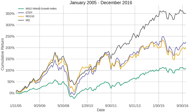
Figure 1. Portfolio performance with GL (global) universe.

FIGURE 2

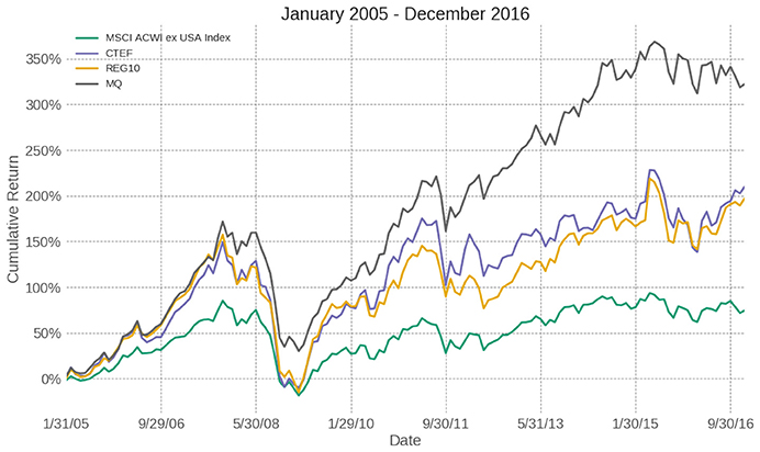
Figure 2. Portfolio performance with XUS (non-US) universe.

FIGURE 3

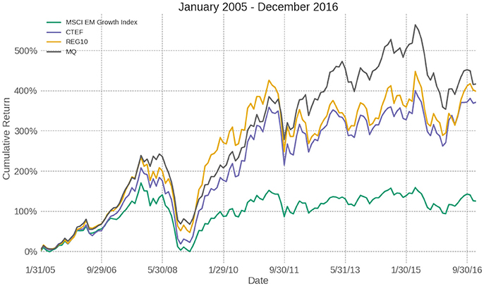
Figure 3. Portfolio performance with EM (Emerging Market) universe.

In Table 1, we report the summary statistics of all these nine portfolios from January 2005 to December 2016. All of these nine Mean-ETL portfolios produce positive active returns over their benchmarks and most of them are statistically significant.

TABLE 1

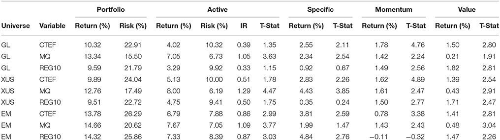
Table 1. Mean-ETL portfolio summary.

Among the three variables, MQ variable performs the best in all of the GL, XUS and EM universes. In the XUS universe, XUS-MQ produces a 8.00% annual active return with an information ratio of 1.29 and a t statistic of 4.47. In the GL stock universe, GL-MQ generates a 7.05% annual active return with an information ratio of 1.05 and a t statistic of 3.63, which is much higher than the GL-CTEF and GL-REG10. As for the EM stock universe, the annual active return of EM-MQ is 7.67% with an information ratio of 1.09 and a t statistic of 3.77. Other than the three stock universes we have studied in this paper, the recent study of Shao [8] reports that the MQ variable in the domestic (US) stock universe generates an active annual return 9.72% with an information ratio of 1.12 and a t statistic of 4.18 during the period of 2000–2013.

As for different universes, the Mean-ETL portfolios perform better in the XUS and EM universes than the GL universe. In the EM stock universe, all of the CTEF, MQ, and REG10 variables generate highly statistically significant active returns: the active returns of EM-MQ, EM-REG10, and EM-CTEF have an information ratio 1.09 (t = 3.77), 0.87 (t = 3.03), and 0.86 (t = 2.99), respectively. While all three variables generate positive active returns over the period of 2005–2016, only the MQ variable generates statistically significant active returns in the GL universe with a t statistic of 3.63.

The “Momentum” factor plays an important role in the portfolios based on the CTEF variable and it contributes highly statistically significant positive returns to the CTEF portfolios. The “Momentum” factor generates positive annual returns of 1.62% (t = 4.89), 1.78% (t = 4.76), and 0.78% (t = 3.38) in XUS-CTEF, GL-CTEF, and EM-CTEF, respectively.

We perform further analyses of the Mean-ETL portfolios based on the MQ variable, which generates the most statistically significant positive active returns. The Axioma attribution of the GL-MQ portfolio is shown in Table 2. In the GL-MQ portfolio, statistically significant positive returns are derived from the “Leverage” factor (debt-to-assets) and “Medium-Term Momentum” (cumulative returns over past 12 months excluding the last month).

TABLE 2

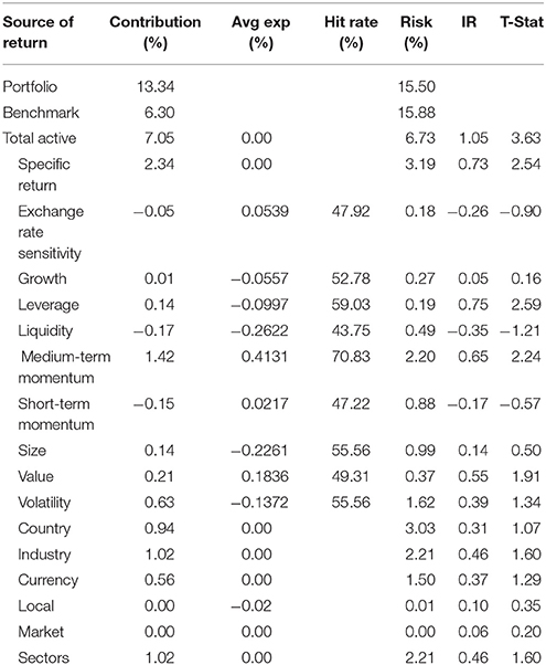
Table 2. Axioma attribution of Mean-ETL-MQ (GL) portfolio.

Table 3 presents the Axioma attribution report of the XUS-MQ portfolio. The “Medium-Term Momentum” factor continues to generate statistically significant positive return: an annual return 1.61% with information ratio of 2.71 and a t statistic of 2.47.

TABLE 3

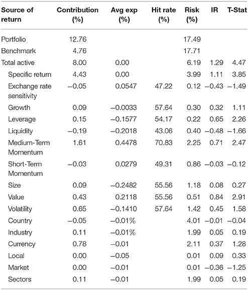
Table 3. Axioma attribution of Mean-ETL-MQ (XUS) portfolio.

The same Axioma analysis of EM-MQ is shown in Table 4. The “Leverage,” “Medium-Term Momentum,” and “Value” factors continue to generate strong positive returns, which are statistically significant. However, the factor that has the highest active return contribution is the “Country” factor, which generates annual return 2.13%, which is much higher than the GL-MQ and XUS-MQ portfolios. The top and bottom five countries in the “Country” factor are shown in Table 5.

TABLE 4

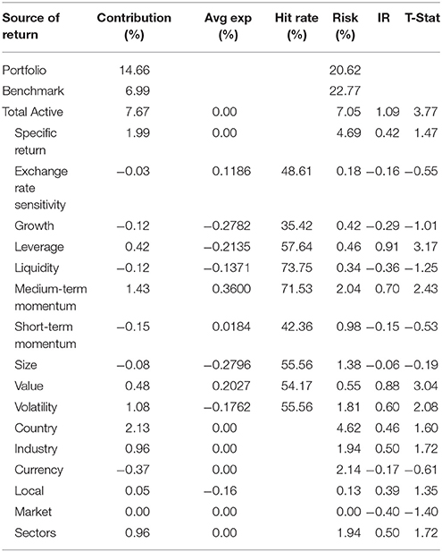
Table 4. Axioma attribution of Mean-ETL-MQ (EM) portfolio.

TABLE 5

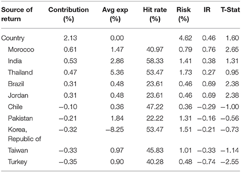
Table 5. Top and Bottom 5 countries in Mean-ETL-MQ (EM) portfolio.

From a practitioner's view, the past performance is not guarantee of future results. The performance of the Mean-ETL portfolios with these variables and universes will be different in the period outside 2005–2016. Like the updates of the original models after 25 years in Guerard [6], we will revisit the robustness of these portfolios with more data in the future.

5. Summary and Conclusions

In this study, we have provided a comprehensive and updated report on the application of the Mean-ETL portfolio framework in portfolio construction when using different fundamental variables and stock universes. Nine portfolios based on three fundamental variables (CTEF, MQ, and REG10) in three universes (GL, XUS, and EM) have been studied and reported. Previous works of the Mean-ETL framework with fundamental variables have been studied with different universes or time periods, and it is difficult to compare the efficiency of different variables. During the period of 2005–2016, we find that the Mean-ETL optimization continues to generate statistically significant active returns with different markets or fundamental variables. In this study, we also find that the MQ variable is a very significant predictor of the stock selection in the Mean-ETL optimization across the three universes (GL, XUS, and EM) during this period. Despite the Mean-ETL portfolios with MQ variable perform better than the other two variables across all three universes in this period, we cannot draw the conclusion that the MQ variable outperforms other variables with different portfolio construction techniques or time periods. For example, Mean-ETL portfolio with CTEF variable outperforms the portfolio with MQ variable in the U.S. stock market in Shao [8].

Author Contributions

The author confirms being the sole contributor of this work and approved it for publication.

Conflict of Interest Statement

BS is employed by Tianyou Asset Management LLC. The views and opinions expressed in this paper are those of the author and do not represent or reflect those of Tianyou Asset Management, LLC.

Acknowledgments

The author thanks Dr. John Guerard and Dr. Svetlozar Rachev for the comments and collaborations on the Mean-ETL optimization. Since our first paper of the Mean-ETL portfolio optimization on the fundamental variables [7] in 2013, we have explored the Mean-ETL methodology with broader universes and different directions. I also thank McKinley Capital Management team to run all the Axioma factor analysis on the portfolios. Any errors remaining are the responsibility of the author.

Footnotes

1. ^This paper is not intended to compare the Mean-Variance and Mean-ETL portfolio optimizations and different portfolio construction methodologies have their own merits.

References

1. Fama EF, French KR. Common risk factors in the returns on stocks and bonds. J Finan Econ. (1993) 33:3–56.

Google Scholar

2. Jegadeesh N, Titman S. Returns to buying winners and selling losers: implications for stock market efficiency. J Finance (1993) 48:65–91.

Google Scholar

3. Guerard JB, Gultekin M, Stone B. The role of fundamental data and analysts' earnings breadth, forecasts, and revisions in the creation of efficient portfolios. Res Finance (1997) 15:69–92.

4. Markowitz H. Portfolio selection. J Finance (1952) 7:77–91.

Google Scholar

5. Guerard JB Jr, Takano M. The development of mean-variance-efficient portfolios in Japan and the US. J Invest. (1992) 1:48–51.

Google Scholar

6. Guerard JB. The development of mean–variance-efficient portfolios in Japan and the United States: 25 years after; or, what has driven stock selection models in Japan and the United States? J Invest. (2017) 26:70–93. doi: 10.3905/joi.2017.26.1.070

CrossRef Full Text | Google Scholar

7. Guerard J, Rachev ST, Shao BP. Efficient global portfolios: big data and investment universes. IBM J Res Dev. (2013) 57:11:1–:11. doi: 10.1147/JRD.2013.2272483

CrossRef Full Text | Google Scholar

8. Shao BP. Mean-ETL portfolio construction in US equity market. In: Guerard JB, editors, Portfolio Construction, Measurement, and Efficiency. New York, NY: Springer International Publishing (2017). p. 155–68.

Google Scholar

9. Graham B, Dodd DL. Security Analysis: Principles and Technique. New York, NY: McGraw-Hill (1934).

10. Elton EJ, Gruber MJ, Gultekin M. Expectations and share prices. Manage Sci. (1981) 27:975–87.

Google Scholar

11. Arnott RD. The use and misuse of consensus earnings. J Portfolio Manage. (1985) 11:18–27.

Google Scholar

12. Guerard JB Jr, Blin J, Bender S. Forecasting earnings composite variables, financial anomalies, and efficient Japanese and US portfolios. Int J Forecast. (1998) 14:255–9.

Google Scholar

13. Shao BP, Rachev ST, Mu Y. Applied mean-ETL optimization in using earnings forecasts. Int J Forecast. (2015) 31:561–7. doi: 10.1016/j.ijforecast.2014.10.005

CrossRef Full Text | Google Scholar

14. Bloch M, Guerard J, Markowitz H, Todd P, Xu G. A comparison of some aspects of the US and Japanese equity markets. Japan World Econ. (1993) 5:3–26.

Google Scholar

15. Guerard JB Jr, Xu G, Gültekin M. Investing with momentum: the past, present, and future. J Invest. (2012) 21:68–80. doi: 10.3905/joi.2012.21.1.068

CrossRef Full Text | Google Scholar

16. Guerard JB. Investing in global markets: big data and applications of robust regression. Front Appl Math Stat. (2016) 1:14. doi: 10.3389/fams.2015.00014

CrossRef Full Text | Google Scholar

17. Guerard JB, Markowitz H, Xu G. Earnings forecasting in a global stock selection model and efficient portfolio construction and management. Int J Forecast. (2015) 31:550–60. doi: 10.1016/j.ijforecast.2014.10.003

CrossRef Full Text | Google Scholar

18. Guerard J, Deng S, Gillam RA, Markowitz H, Xu G, Wang Z. Investing in Global Equity Markets with Particular Emphasis on Chinese Stocks. (2016). Available online at: https://ssrn.com/abstract=2744304

19. Rachev ST, Martin RD, Racheva B, Stoyanov S. Stable ETL optimal portfolios and extreme risk management. In: Bol G, Rachev ST, Würth R, editors, Risk assessment. New York, NY: Springer (2009). p. 235–62.

Google Scholar

20. Artzner P, Delbaen F, Eber JM, Heath D. Coherent measures of risk. Math Finance (1999) 9:203–28.

Google Scholar

21. Rockafellar RT, Uryasev S. Optimization of conditional value-at-risk. J Risk (2000) 2:21–42. doi: 10.21314/JOR.2000.038

CrossRef Full Text | Google Scholar

22. Shao BP, Rachev ST. Mean-ETL optimization of a global portfolio. J Invest. (2013) 22:115–9. doi: 10.3905/joi.2013.22.4.115

CrossRef Full Text | Google Scholar