Interpretable Multiclass Models for Corporate Credit Rating Capable of Expressing Doubt

Corporate credit rating is a process to classify commercial enterprises based on their creditworthiness. Machine learning algorithms can construct classification models, but in general they do not tend to be 100% accurate. Since they can be used as decision support for experts, interpretable models are desirable. Unfortunately, interpretable models are provided by only few machine learners. Furthermore, credit rating often is a multiclass problem with more than two rating classes. Due to this fact, multiclass classification is often achieved via meta-algorithms using multiple binary learners. However, most state-of-the-art meta-algorithms destroy the interpretability of binary models. In this study, we present Thresholder, a binary interpretable threshold-based disjunctive normal form (DNF) learning algorithm in addition to modifications of popular multiclass meta-algorithms which maintain the interpretability of our binary classifier. Furthermore, we present an approach to express doubt in the decision of our model. Performance and model size are compared with other interpretable approaches for learning DNFs (RIPPER) and decision trees (C4.5) as well as non-interpretable models like random forests, artificial neural networks, and support vector machines. We evaluate their performances on three real-life data sets divided into three rating classes. In this case study all threshold-based and interpretable models perform equally well and significantly better than other methods. Our new Thresholder algorithm builds the smallest models while its performance is as good as the best methods of our case study. Furthermore, Thresholder marks many potential misclassifications in advance with a doubt label without increasing the classification error.

1. Introduction

The evaluation of the economic situation of commercial enterprises is an important task because inaccurate predictions may lead to huge financial losses. Machine learning methods using annual accounts offer an automated and objective way to achieve high prediction rates for this task. In any case, machine learning models may be incorrect. Therefore, these models cannot completely replace expensive experts. Thus, our goal is to build objective models with a low prediction error as a helpful decision support for experts in credit rating. Therefore, we additionally focus on the interpretability of models. There are binary tasks such as insolvency prediction and multiclass tasks like credit rating. In machine learning, the latter case is often reduced to several binary learning steps. This might change the structure and increase the complexity and size of the models and therefore may destroy their interpretability.

In the literature, the definitions for interpretability in terms of machine learning are different. A model is called interpretable if the importance of features is derivable [1] or if it consists entirely of interpretable rules, no matter how many there are [2]. We suggest in our recently published study [3] that interpretable models need to be interpretable by human beings and therefore should consist entirely of interpretable rules, but of a reasonable amount. Furthermore, these rules have to be connected by interpretable operations. The less rules there are in a model the more interpretable it becomes. The rules should have a structure of what a human being would think of: Boolean expressions with threshold indicators. In this work, a threshold indicator is the Boolean indicator function of a threshold of a financial ratio.

The question may arise why models need to be interpretable and why not simply apply black-box models with a high accuracy. Florez-Lopez and Ramon-Jeronimo [2] listed three important benefits from interpretable models.

• Interpretable models allow to justify the decision of a refused credit [4, 5] which is actually a legal obligation in some countries, e.g., in the UK and the US [6].

• Managers are less likely to refuse to use a model which they understand [7]

• Models that are understood can be combined with expert knowledge to obtain a more powerful model [8].

Sometimes the prediction for some instances may be of a high uncertainty. In some applications, it would be helpful to have an I-Dont-Know-classification (IDK) label for these instances to express doubt rather than guessing a label. These IDK-classified instances can be treated in a more sophisticated or expensive process. In insolvency prediction, for example, if an enterprise is labeled solvent with a high uncertainty, the possibility to lose the money of a granted credit to this enterprise can be reduced by manually reevaluating this enterprise again by experts. Technically, IDK-classifications are simply an additional class label which does not occur in the training set. Therefore, each multiclass model can represent IDK-classifications. There are several challenges when dealing with IDK-classifications, like the training process where none of these labels are observed, finding a reasonable amount of IDK-classifications, and using a decent error measure when evaluating the performance.

We further developed our binary Thresholder algorithm for learning Disjunctive Normal Forms (DNFs) to output interpretable multiclass models which can express doubt and compared it with another DNF and Decision Tree (DT) algorithm. We compared these three interpretable models with some of the most popular and recently used non-interpretable methods as well, namely Random Forests (RFs), Artificial Neural Networks (ANNs), and Support Vector Machines (SVMs).

In a binary learning setting to predict insolvency we already showed non-inferiority for interpretable models [3]. In this paper we want to show that this does not only work for a multiclass problem, but even better for a problem with man-made classifications, i.e., credit ratings. Our main finding is that the interpretable models outperform the more sophisticated black-box models in our case study on credit rating. This can be explained by the nature of the problem. Insolvency is influenced by multiple economic factors. In contrast, credit rating is based on decisions by people thinking in interpretable ways. Thus, we assume that logical operations on threshold indicators for financial ratios are the best choice to reconstruct human decisions in credit rating. Furthermore, we introduce Thresholder for interpretable multiclass models which additionally offers the possibility to express doubt.

The remainder of this paper starts with Section 2 where related work is presented. The utilized learning algorithms and multiclass methods are described in Section 3. Afterwards, we present the case study in Section 4 whose results are presented and discussed in Section 5. Finally, Section 6 concludes this paper with a brief summary of the main contributions of this paper and an outlook on future work.

2. Related Work

There are several binary classification problems in finance, e.g., predicting bankruptcy, insolvency, business failure, or financial distress. Credit rating or bond rating with more than two classes are typical multiclass classification problems. However, there are many studies which examine these problems for only two classes.

Most studies are solely based on data obtained from annual accounts. Despite the fact that few studies also consider qualitative factors [9], this paper focuses on quantitative data. A common problem is acquiring useful data sets since annual accounts of enterprises have to be collected from different sources, declarations of insolvency are only published for a limited amount of time, and rating classes which are not publicly available are determined by credit rating agencies. Therefore, many studies suffer from small and different data sets as well. Thus, their absolute results are not directly comparable. A second problem of most data sets are big imbalances. Naturally, there are less insolvent or low rated enterprises for a given time period than solvent ones. Inhomogeneities are a third problem. Predictions for a mixture of enterprises of different sizes, of different industries, and with annual accounts from different years are more difficult than they are for homogeneous data sets.

In the following, we provide a short overview of general statistical and machine learning methods, methods for multiclass problems, and interpretable models in finance.

2.1. Machine Learning in Finance in General

The following is a short overview about prior studies on binary financial problems using statistical and machine learning approaches. It shows which methods are used and that in most studies at least one of the data problems stated above is present.

One of the first studies on business failure uses an univariate model [10]. Afterwards, rather simple methods like (linear) Multiple Discriminant Analysiss (MDAs) [11–13], logit models [14–16], and probit models [17, 18] were used.

Later, these simple methods were outperformed and replaced by the very famous ANNs [19–22] and SVMs [23–26]. Both are the most popular methods to the present day.

An alternative to the two black-box methods above are interpretable methods like DTs [27, 28], Regression trees [29], Rough Set Theory (RST) [30–32], and DNFs [33–35] which are also referred to as rule sets. Especially newer studies yield comparable results to SVMs and ANNs.

The newest approaches mainly concentrate on ensemble learning algorithms in combination with boosting and bagging [36–41] to increase the performance of existing algorithms.

A detailed overview of the history of methods used on business data can be found in Balcaen and Ooghe [42] and Dimitras et al. [43]. A general survey on bagging and other ensemble techniques in bankruptcy prediction can be found in Verikas et al. [44].

2.2. Machine Learning in Finance for Multiclass Credit Rating

Most of the studies on multiclass credit rating propose SVMs or ANNs. However, interpretable DNFs or DTs are hardly ever considered.

Huang et al. [45] performed a credit rating comparing methods for improved accuracy of SVMs and improved interpretability through feature extraction for ANNs. However, they realized that only a slight performance improvement of SVMs was achieved. They worked with five different rating classes.

Instead of a credit rating a bond rating with six classes was done by Cao et al. [46]. They tested different multiclass methods for SVMs and compared these results with ANNs and logit models. A main finding was that few features are not only sufficient, but can even improve the accuracy. They achieved an accuracy gain of about 2%.

Hájek [47] proposed different ANNs for municipal credit rating and compared them with classification trees and SVMs. Probabilistic neural networks obtained the best results. However, the interpretable classification trees achieved good results as well. They used four and nine classes and concluded that only small lists of features determine the classification.

Kim and Ahn [48] performed a credit rating with four classes. They propose new multiclass methods for SVMs and compare them with other methods. Their method outperformed the rest, but only with an advantage of less than 1%.

Guo et al. [49] studied credit rating with four classes as well. They used a support vector domain combined with a fuzzy clustering algorithm and compared it with different SVM multiclass methods. Their approach outperformed conventional multiclass methods with less than 2%.

A credit rating with 16 classes was performed by Kwon et al. [50]. They used double ensemble approaches containing bagging and boosting to significantly improve DTs.

2.3. Interpretable Models in Finance

There are general approaches that try to simplify non-interpretable models. They render models interpretable by extracting rules or pointing out feature importance. Some approaches combine interpretable models to a more accurate but bigger interpretable model.

There are approaches to make ANNs more interpretable [4, 51–55]. Some approaches try to simplify black-box models like SVMs [56] and show interpretations for single data points or extract rules as well [57, 58]. These approaches try to extract rules which do only represent an approximation of the original model. This decreases the accuracy of the models. Some researchers combine interpretable rules [1, 2] to achieve better results of interpretable models. For all methods above there is a tradeoff between accuracy and interpretability. Models gain accuracy by getting bigger and thus lose interpretability. Vice versa, non-interpretable models lose accuracy by becoming interpretable. Although, the loss in accuracy often is very small.

In finance, most studies concentrate on improving the prediction accuracy. There are few studies dealing with interpretability of models, especially for multiclass problems. One of these studies was performed by Kim et al. [59] on a small data set to predict six class bond rating. They compared DTs, ANNs, MDAs, and logit models. ANNs performed much better than the rest. However, this study dates back to 1993, the data set is very small, and DT algorithms have evolved a lot since then. As mentioned above, Huang et al. [45] improved interpretability in credit rating through feature extraction for ANNs.

For binary problems in finance, research has shown that already existing interpretable models are not necessarily worse than more complex models. Jones et al. [60] concluded that simpler and more interpretable classifiers like logit, probit, and MDAs performed comparatively well to ANNs and SVMs when predicting rating changes. Virág and Nyitrai [61] studied RST for bankruptcy prediction. They showed that this interpretable model is competitive to ANNs and SVMs. We showed in a prior study [3] that interpretable models are not inferior to black-box models in insolvency prediction, by comparing DTs, DNFs, RFs, ANNs, and SVMs.

On a final note, Hand [5] argues that “the apparent superiority of more sophisticated methods may be something of an illusion.” He showed that for many cases the marginal gain of sophisticated and ensemble models is small compared to simple models. Section 2.2 shows similar observations for most multiclass credit rating studies. Nevertheless, we appreciate the work on sophisticated methods because classification performance is still a more important factor for a classifier than interpretability.

In this study, we examine interpretable multiclass models for a three-class credit rating. We consider the interpretable model classes of DTs and DNFs using different learning algorithms to build the models. The model size is restricted to obtain small and interpretable models. We compare them with the most common methods, namely ANNs and SVMs. RFs are used to represent combined interpretable models using thresholds. We compare the multiclass methods used by Guo et al. [49] and an ensemble method representatively for the work of Kwon et al. [50]. Furthermore, we use our new approach to express doubt in the classification. Three data sets with annual accounts of 1256 trading, 1361 construction, and 1066 financial enterprises are used for a three-class credit rating.

3. Methods Used for Credit Rating

In this paper, the following models are studied:

• Thresholder DNFs,

• RIPPER DNFs,

• C4.5 DTs,

• RBF-networks (ANNs),

• RFs,

• Linear SVMs (L-SVMs),

• RBF-kernel SVMs (R-SVMs), and

• Polynomial-kernel SVMs (P-SVMs).

In this section, we describe the three interpretable already published (binary) learning algorithms for DNFs and DTs in detail. Afterwards, there will be description of common multiclass methods, followed by a discussion of their interpretability. At last, we present our new multiclass approach to obtain interpretable multiclass models using Thresholder. The Thresholder algorithm and the multiclass methods were implemented by us. For the other algorithms the implementation of the WEKA learning framework [62] was used.

3.1. Known Interpretable Learning Algorithms Used

We use three algorithms to build interpretable models; our Thresholder algorithm, as well as the RIPPER algorithm to build DNFs, and the famous C4.5 algorithm to build DTs.

A DNF is a disjunction of monomials m with a conjunction of literals l

$\begin{array}{l}DNF=m_1\vee m_2\vee \dots \vee m_r\hfill \\ =(l_{1,1}\wedge l_{1,2}\wedge \dots \wedge {\text{l}}_{1,p}\text{)}\hfill \\ \vee (l_{2,1}\wedge l_{2,2}\wedge \dots \wedge l_{2,p})\hfill \\ \vee \dots \hfill \\ \vee (l_{r,1}\wedge l_{r,2}\wedge \dots \wedge l_{r,p}),\hfill \end{array}$

with r monomials and p literals per monomial. We call these literals threshold indicators. If this formula is fulfilled, the instance will be classified positive, otherwise negative. The literature calls DNFs rulesets as well and the containing monomials rules. This is likewise correct, but less precise as well.

A DT is a binary tree with threshold indicators as nodes which split the input space. The leaves determine the classification.

3.1.1. Thresholder Algorithm for Learning DNFs

We have recently published the binary classification version of this Thresholder algorithm [3] so we provide only a short overview. This algorithm is a greedy heuristic and calculates a DNF model of threshold indicators. In the base algorithm, each monomial's threshold is calculated step by step. This is achieved by considering each feature value of the instances as a possible upper and lower threshold candidate and selecting the best one. If all p thresholds are calculated or there is no further benefit in adding thresholds, the algorithm builds the next monomial.

We improved this greedy approach using a semi-greedy algorithm. For each monomial in the DNF, we calculate n monomial candidates m₁, m₂, …, m_n simultaneously, with the first threshold indicator of dimension 1, 2, …, n. The following threshold indicators of each monomial candidate are calculated greedy as before. The best of these n monomial candidates is added as monomial to the DNF. This decision is made according to the classification error of the DNF using this monomial candidate. Afterwards, the next monomial is calculated in the same way.

To further improve the heuristic, we use post-pruning which is adapted from the C4.5 DT algorithm. We build a bigger DNF than intended and afterwards prune some threshold indicators to obtain a different DNF. Like the improvement above, this technique should compensate for the greediness of the approach. The process of building the DNF involves adding one literal after another. In contrast, the pruning technique deletes multiple literals at any position in the DNF. Our pruning technique has three parameters pruning complexity p_c, pruning error p_e, and pruning size p_s and works as follows: remove the set of 1…p_c threshold indicators or the monomial, whichever worsens the error of the model at least. Repeat this until the error worsens by at most p_e. Depending on the value of p_e, this might increase the training error slightly, but decreases overfitting and therefore might decrease the generalization error. The third parameter p_s restricts the maximum size of the model measured by the number of threshold indicators. Pruning will not stop until model size is equal or below p_s. This parameter controls the degree of interpretability. For reducing the generalization error, these pruning parameters should be selected on a separate data set.

There are several generalization parameters which also allow for the output models to be adjusted to one's needs. The maximum number of literals and monomials is adjustable, as well as the pruning parameters allowing to output models of a certain size.

This algorithm was already successfully used in this form for a binary problem [3]. For this study, we applied only a few improvements for the pruning part. Further, we added parameter p_s that prunes the DNF until a certain model size is reached. Especially for small values of p_s, it is important to prune the DNF to exactly size p_s + p_c and, afterwards, to prune the remaining p_c literals all at once. This enhances the performance and minimizes the influence of the greediness of the pruning algorithm. Additionally, the option to prune a monomial as a whole was added. We added some performance improvements as well such as lowering p_c for bigger model sizes because it exponentially increases computation time with regard to the model size.

3.1.2. RIPPER Algorithm for Learning DNFs

Repeated Incremental Pruning to Produce Error Reduction (RIPPER) is an improvement to IREP [63] and was introduced by Cohen [64]. RIPPER is a greedy heuristic, which grows monomials, prunes them, and then adds them to a DNF. To achieve this, the training set is randomly partitioned into a growing set and a pruning set. After that, one monomial at a time is calculated, using the growing set. The selection of literals is based on the metric precision - false discovery rate. After a monomial is calculated, it is pruned using the pruning set and accuracy as the performance measure. The pruned monomial is added to the DNF. Instances covered by the monomial are deleted. The heuristic stops, if all positive instances are covered or the description length of the DNF is more than a certain parameter larger than the smallest description length of the monomials obtained so far. The DNF is post-processed in an optimization phase, which optimizes the monomials step by step by creating a replacement and a revision of the monomial. The replacement is created by growing and then pruning a new rule, where pruning minimizes the error of the entire DNF. The revision is created the same way, but starts with the original rule instead of an empty rule. A decision is made by the minimum description length (MDL) heuristic [65], whether the original monomial should or should not be exchanged by the replacement or the revision.

Important parameters are the number of folds which are used for pruning and the generalization parameter which determines the minimum number of instances in a rule.

3.1.3. C4.5 Algorithm for Learning DTs

C4.5 is a widely used DT algorithm developed by Quinlan [66] based on the ID3 algorithm [67]. The information gain criterion is used to split the data by creating the nodes of the tree. After it is grown, the tree is pruned by remove branches which are not helpful for the classification. This avoids overfitting and reduces the size of the model.

Important generalization parameters are the confidence factor which controls the amount of pruning and the minimum number of instances in a leaf.

3.2. Known Multiclass Meta-Algorithms Used

Multiclass classification problems have more than two different label values for their classes. Many learning algorithms naturally support only binary classification, like SVMs. However, there are meta-algorithms which turn binary learning algorithms to multiclass classifiers by using multiple binary learning algorithms.

3.2.1. All-at-once

Some classifiers naturally support training multiple classes all at once. Tree-based models like DTs and RFs can assign arbitrary label values in their leaves. Since DNFs are Boolean expressions, they naturally support only binary classification. ANNs classify multiple classes by using multiple output nodes with a probability for each label. SVMs cannot handle multiclass learning problems naturally.

3.2.2. One-vs-one

This method [68] combines binary classifiers to multiclass classifiers and therefore naturally allows binary classifiers like SVMs to be used for multiclass problems. There are classifiers trained for each pair of labels resulting in $\frac{l(l-1)}{2}$ classifiers where l is the number of labels. For an ordinal multiclass problem, each label c_i is trained against each label c_j > c_i. The predicted label is a majority vote of the $\frac{l(l-1)}{2}$ classifiers. In case of a tie, a decision must be made, e.g., by using the smaller class index.

3.2.3. One-vs-rest

Like the one-vs-one method, this method trains multiple binary classifiers [69]. There is one classifier trained for each label. Each label c_i = 1…l is trained against the rest. Again, the final decision is a majority vote of all classifiers. If label c_i wins against the rest, it gets a vote. Again, the final decision is a majority vote.

Compared to one-vs-one, an advantage of this method is the smaller runtime which is linear in the number of labels. On the contrary, the binary training is more expensive, because the training set consists of the whole data set. A disadvantage is the imbalance between the data of label c_i and the data of the merged rest in the training set where in general the latter is probably much bigger. Furthermore, it is problematic that for this method a tie is much more likely than for the one-vs-one method, because a label can only get either one or no vote. This problem can be solved by using probability estimates for each class as a vote.

3.2.4. One-vs-next

One-vs-next and one-vs-followers (explained below) are both methods for ordinal multiclass problems. Originally, Kwon et al. [70] proposed this method for ANNs. Later, this method was adopted for other methods like SVMs [48].

The idea is to train l − 1 classifiers to differentiate between label c_i and c_i−1 for c_i = l … 1. If the first classifier decides for the higher class, then this will be the final classification. However, if the classifier decides for the lower class, the next classifier will be evaluated. This is repeated until either the higher classification is chosen or the last classifier is evaluated with a final decision. Advantages of this method are fewer classifiers and balanced data sets. Furthermore, this method preserves interpretability of interpretable binary classifiers by simply cascading them.

3.2.5. One-vs-followers

Like the one-vs-next approach, this method works on ordinal multiclass problems. The difference is what label c_i is compared to. It is not only compared to c_i−1, but to all labels c_j = i − 1…0. This leads to the same amount of classifiers. Similarly to the one-vs-rest approach it leads to imbalanced training data sets. This method also maintains interpretability since it uses the same hypothesis class as the one-vs-next method.

3.3. New Thresholder Algorithm for Learning Cascaded DNFs

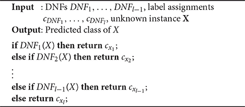
As mentioned above, DTs are naturally interpretable multiclass classifier. Interpretable DNF multiclass classification can be obtained by cascading number of labels l − 1 binary DNF classifiers which classify one class with one DNF consecutively. This cascade of DNFs can be seen as a decision list of DNFs. Algorithm 1 shows how such a classification is achieved. Since this model is basically an interpretable decision list which grows only linearly in size with the number of class labels, it can be considered an interpretable multiclass model.

RIPPER uses this model for multiclass classification. To build such a classifier, the algorithm orders the classes of the data set ascending by their size c₁, …, c_l and trains DNF₁, …, DNF_l−1 using labels c₁, …, c_l−1 as positive data and labels ⋃(c_i, i > 1), …, ⋃(c_i, i > l − 1) as negative data. The training leads to a cascaded DNF as described in Algorithm 1. This method is basically the one-vs-followers approach with a different class ordering.

ALGORITHM 1

Algorithm 1. Cascaded DNF classifier.

3.3.1. Learning Cascaded DNFs

For our Thresholder algorithm we use all multiclass strategies from Section 3.2 and convert them into an interpretable form. As mentioned above, the one-vs-next and one-vs-followers approaches already yield an interpretable form since they are trained according to Algorithm 1 with an ordering of class labels. The one-vs-one and one-vs-rest approaches are more difficult because the resulting majority votes consist of interpretable parts, but the whole classifiers are not interpretable, like RFs. In our approach, we solve this problem by transforming them into cascaded DNFs. We achieve this by using Boolean algebra to calculate conjunctions and negations of DNFs. Before we explain this algorithm in detail, we show how applying these two operations on DNFs will maintain the DNFs every time.

3.3.1.1. Conjunctions and negations of DNFs

The conjunction of two DNFs can be transformed back into a single DNF using the distributive property and the associative property of Boolean algebra as seen below. The disjunction of two DNFs is automatically a disjunction of all monomials and therefore a new DNF.

$\begin{array}{l}DN{F}_1\vee DN{F}_2\hfill \\ =(m_l\vee \dots \vee m_r)\vee ({m^{\prime }}_1\vee \dots \vee {m^{\prime }}_2)\hfill \\ =DN{F}_{1\vee 2}\hfill \end{array}$

The conjunction of a DNF and a literal is a new DNF with a conjunction of this literal with each monomial.

$\begin{array}{l}l\wedge DN{F}_1\hfill \\ =l\wedge (m_1\vee \dots \vee m_r)\hfill \\ =(l\wedge m_1)\vee \dots \vee (l\wedge m_r)\hfill \\ =(l\wedge l_{1,1}\wedge \dots \wedge l_{1,p})\vee \dots \vee (l\wedge l_{r,1}\wedge \dots \wedge l_{r,p})\hfill \\ =DN{F}_{l\wedge 1}\hfill \end{array}$

Using the two formulae above, the conjunction of two DNFs can be transformed into a single DNF.

$\begin{array}{l}DN{F}_1\wedge DN{F}_2\hfill \\ =(m_1\vee \dots \vee m_r)\wedge DN{F}_2\hfill \\ =(m_1\wedge DN{F}_2)\vee \dots \vee (m_r\wedge DN{F}_2)\hfill \\ =\left((l_{1,1}\wedge \dots \wedge l_{1,p})\wedge DN{F}_2\right)\vee \dots \vee \hfill \\ \left((l_{r,1}\wedge \dots \wedge l_{r,p})\wedge DN{F}_2\right)\hfill \\ =\left(l_{1,1}\wedge \dots \wedge (l_{1,p}\wedge DN{F}_2)\right)\vee \dots \vee \hfill \\ \left(l_{r,1}\wedge \dots \wedge (l_{r,p}\wedge DN{F}_2)\right)\hfill \\ =DN{F}_{1\wedge 2}\hfill \end{array}$

The negation of a DNF can be calculated using De Morgan's and distributive laws as seen below. Threshold indicators can be negated by inverting the relational operator, i.e., changing “>” to “≤” and vice versa. Using this, the negation of a monomial can be calculated.

$\begin{array}{l}\overline{m_1}\hfill \\ =\overline{(l_{1,1}\wedge \dots \wedge l_{1,p})}\hfill \\ =(\overline{l_{1,1}}\vee \dots \vee \overline{l_{1,p}})\hfill \end{array}$

The conjunction of two negated monomials can be transformed into a DNF by using every combination of one literal per monomial as a new monomial.

$\begin{array}{l}\overline{m_1}\wedge \overline{m_2}\hfill \\ =(\overline{l_{1,1}}\vee \dots \vee \overline{l_{1,p}})\wedge (\overline{l_{2,1}}\vee \dots \vee \overline{l_{2,p}})\hfill \\ =(\overline{l_{1,1}}\wedge \overline{l_{2,1}})\vee \dots \vee (\overline{l_{1,1}}\wedge \overline{l_{2,p}})\vee \dots \vee \hfill \\ (\overline{l_{1,p}}\wedge \overline{l_{2,1}})\vee \dots \vee (\overline{l_{1,p}}\wedge \overline{l_{2,p}})\hfill \end{array}$

And finally, the negation of a DNF, which is a conjunctive normal form, can be transformed into a DNF as well using the formulae above.

$\begin{array}{l}\overline{DN{F}_1}\hfill \\ =\overline{m_1\vee \dots \vee m_r}\hfill \\ =\overline{m_1}\wedge \dots \wedge \overline{m_r}\hfill \\ =DN{F}_{\overline{1}}\hfill \end{array}$

Calculating the conjunction or negation of a DNF exponentially increases the amount of threshold indicators, a problem which will be addressed later in Section 3.3.1.3.

3.3.1.2. Interpretable one-vs-one and one-vs-rest classifiers

Since the data sets of our case study have three classes, we explain our algorithm only for the three class case for reasons of simplicity. However, it can easily be extended to n classes.

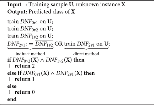
We denote DNF_ivj the binary classifier which is trained with label j as positive and label i as negative data. Taking an instance of the data set as parameter, it returns true for label j and false for label i. The majority vote of the three one-vs-one classifiers DNF_0v1, DNF_0v2, and DNF_1v2 votes for label 2 only if DNF_0v2 and DNF_1v2 both return true. It votes for label 1 only if DNF_0v1 and $DN{F}_{2v1}=\overline{DN{F}_{1v2}}$ both return true. It votes for label 0 if DNF_0v1 and DNF_0v2 both return false. Otherwise, there is a tie. In this case we assign label 0 as well.

Firstly, we train DNF_0v1, DNF_0v2, and DNF_1v2 similar to the normal one-vs-one approach. Afterwards, we build two cascaded DNFs using the conjunctions and negations of DNFs representing the majority votes as seen above. An alternative method is to directly train the negated DNF from the data instead of calculating it. This requires one additional training step. Both methods are shown in Algorithm 2.

ALGORITHM 2

Algorithm 2. Indirect and direct method for interpretable one-vs-one DNF classifiers.

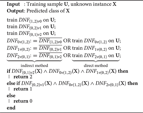
We denote DNF_{(i, j)vk} the binary classifier which is trained with label i and j as negative and label k as positive data. Taking an instance of the data set as parameter, it returns true for label k and false for label i or j. The interpretable one-vs-rest classifier returns a positive classification for class k only if DNF_{(i, j)vk} returns true, DNF_{(k, i)vj} returns false, and DNF_{(j, k)vi} returns false. Like the interpretable one-vs-one method, this method exists in an indirect and direct version. Algorithm 3 shows this procedure in detail.

ALGORITHM 3

Algorithm 3. Indirect and direct method for interpretable one-vs-rest DNF classifiers.

3.3.1.3. Simplification and pruning of cascaded DNFs

As mentioned above, the conjunction and negation operations for DNFs increase the size of the resulting cascaded DNFs exponentially, a problem which does not exist for directly calculated models from the one-vs-next and one-vs-followers approaches. However, in these bigger DNFs, many rules are redundant and can be pruned for simplification.

If a monomial contains multiple threshold indicators of the same dimension and orientation, the less restrictive ones can be discarded without changing the logic of the Boolean formula. In this example, the first threshold indicator can be discarded

$\begin{array}{l}\text{Solvent}=((\text{Cash}\text{flow}>1.45\text{mil}.€)\wedge \hfill \\ (\text{Cash}\text{flow}>1.5\text{mil}.€)\wedge \hfill \\ (\text{RoI}>9.5\%))\hfill \\ \vee \dots .\hfill \end{array}$

Whole monomials can be discarded as well; consider the example of the conjunction of two monomials m₁ and m₂, where m₁ is less restrictive than m₂ in every threshold

$\begin{array}{l}\text{Solvent}=((\text{Cash}\text{flow}>1.45\text{mil}.€)\wedge (\text{RoI}>9.5\%))\hfill \\ \vee ((\text{Cash}\text{flow}>1.5\text{mil}.€)\wedge (\text{RoI}>10\%))\hfill \\ \vee \dots .\hfill \end{array}$

Then, m₂ can be pruned and m₁ already represents the conjunction.

Using these conversions, which do not touch the outcome of the formulae, the size of the cascaded DNF shrinks significantly. Nevertheless, the model size might become clearly bigger than directly calculated models since there might be monomials which are not exactly as restrictive, but only almost as restrictive as other monomials

$\begin{array}{l}\text{Solvent}=((\text{Cash}\text{flow}>1.45\text{mil}.€)\wedge (\text{RoI}>9.5\%))\hfill \\ \vee ((\text{Cash}\text{flow}>1.4\text{mil}.€)\wedge (\text{RoI}>10\%))\hfill \\ \vee \dots .\end{array}$

Pruning them would change the logic of the formula, but in practice this might only affect very few instances indicating the usage of post pruning. Therefore, we apply the same pruning algorithm for both a single DNF and the cascaded DNF classifier.

After all, we have six interpretable multiclass methods implemented for our Thresholder algorithm, namely

• one-vs-next,

• one-vs-followers,

• one-vs-one(-indirect),

• one-vs-one-direct,

• one-vs-rest(-indirect), and

• one-vs-rest-direct.

All of these methods are trained with an ascending and descending order of the class labels in a three-fold-cross-validation of the training data to chose the better order. The all-at-once method of our Thresholder trains all of the six methods above in a three-fold-cross-validation and chooses the best one. When there is a tie, it chooses the one with the smaller model size.

3.3.2. IDK-Classification for Cascaded DNFs

IDK-labels are assigned by classifiers, but cannot be observed in training data sets. We propose to assign IDK-classifications when a tie of the one-vs-one and one-vs-rest multiclass method occurs. Therefore, all classifiers using these methods can implement IDK-classification.

However, we want to go one step further and develop interpretable models using IDK-classifications. In the previous section, we presented interpretable one-vs-one and one-vs-rest multiclass methods for Thresholder. We assign the label 0 in case of a tie. However, if we add an l-th DNF to our cascade, we can distinguish between label 0 and a tie which we can assign an IDK-classification. Algorithm 4 shows this procedure for the one-vs-one method. IDK-classification using the one-vs-rest method works similar.

The all-at-once method of Thresholder using IDK-classifications uses only the four multiclass methods which support IDK-classifications, i.e., the two versions of one-vs-one and one-vs-rest.

ALGORITHM 4

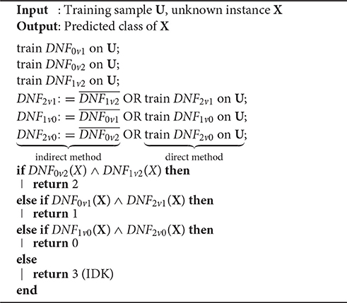
Algorithm 4. Indirect and direct method for interpretable one-vs-one DNF classifiers using IDK-classifications.

Compared to the basic one-vs-one method, the model size is increased by one additional DNF and the training involves negating or training two additional DNFs. As before, the model size can be controlled via pruning. Furthermore, using different values of τ, pruning can control the amount of IDK-assignments. Decreasing τ should result in an increase of IDK-classifications and an increase of the classification error.

4. Case Study

This section describes the database which we use for credit rating. It addresses the experiments we ran, the settings we used and the process of evaluation.

4.1. Data

This case study is based on the DAFNE database by the credit bureau [71]. In our previous study on insolvency prediction [3], we worked with a much older version of this database with a big number of inhomogeneous enterprises of different industries, sizes, and years of annual accounts. This time we obtained more homogeneous data. Thus, we were able to work with a random selection of three separate data sets roughly containing 1000 to 1500 enterprises of the industries wholesale and retail trade, construction, and finance. Each data set contains mostly German and only very big enterprises¹ with annual accounts from 2013 divided into three rating classes. The highest rating matches Standard and Poor's AAA to BB+ rating classes, the medium rating matches BB to B, and the lowest rating matches B− to D. The idea was to find 500 enterprises for each industry and rating class, but since enterprises with the lowest rating are comparatively rare, this requirement could not be met. Details about the actual numbers can be found in Table 1.

TABLE 1

Table 1. Number of enterprises of each rating class as they appear in our data sets.

The features of the data sets are directly taken or calculated from annual accounts, i.e., balance sheets and income statements. Many of these features contain missing values since only a few financial ratios are required to be published in an annual financial statement. We discarded all features that were not at least 90% complete. All features which were not used in our previous study [3] and which are just single values from balance sheets or income statements were discarded as well. Performing this feature selection, we ended up with nine financial ratios as shown in Table 2.

TABLE 2

Table 2. The nine financial ratios used in this study.

The missing values had to be replaced with some numerical values. Experiments with different replacement strategies have shown that missing values provide rating information. Enterprises with a low rating tend to have more missing values. Therefore, our replacement strategy for missing values is using the value zero instead of mean, median or other estimators. This value isolates the information and can easily be recognized in the resulting model. Our data sets are randomly drawn subsets of bigger data sets of the Creditreform. Thus, the distribution of missing values should represent the distribution of the missing values of the bigger data sets. Since this distribution is not altered, missing values are a legitimate discrimination criterion.

4.2. Experiments

We have chosen the classification error as a performance measure. According to the related literature this is a common measure for multiclass problems in finance. Since the data is split randomly, repetitions slightly change results. Therefore, we performed 20 repetitions and took the mean value of these results. Then we tested the statistical significance between the different methods using Welch's t-test [72] and the Wilcoxon signed-rank test [73] for pairwise error and model size comparisons. We denoted results as significantly different, if the p-value was below 0.01.

For the error rate in case of IDK-classifications, we use a parameter τ to penalize assignments of this class. As stated by Alpaydin [74], choosing τ = 0, an IDK-classification is always assigned. Choosing τ = 1, an IDK-classification is never assigned. Therefore, the parameter should be chosen that 0 < τ < 1. Therefore, we have chosen τ = 0.67, i.e., the probability of guessing the wrong label in the three class case.

There are different measures for the model size of DNFs and DTs. The size of a DT can be measured by the size of the tree which is the number of nodes (threshold indicators) and the number of leaves (output values). This measure is used in WEKA as well [62]. Possible measures for the DNF size are the number of rules as used in WEKA [62] and the total number of threshold indicators [75]². Since the first measure only counts the number of monomials and does not take the size of the monomials into account at all, we consider the second measure to be more appropriate to quantify model size and interpretability. However, simply using the latter measure for cascaded DNFs would result in an unfair advantage over DTs. Hence, we have to add the number of output values which is the number of single DNFs +1.

The algorithms from Section 3.1 were evaluated using the standard procedure which splits the data randomly into a 67% training and 33% test split. Since standard parameters are not always the best choice, a three-fold cross-validation was applied to the training set for the parameter selection of all algorithms.

We evaluated all learning algorithms of Section 3.1 in combination with all multiclass methods from Section 3.2. The one-vs-one and one-vs-rest methods were applied in two different ways. Thresholder used the indirect and direct method (Section 3.3.1.2). All other algorithms used the normal method with majority votes and a modified method with probability estimates as votes. To test whether the learning algorithms can be further improved by ensemble learning, we exemplarily tested the one-vs-one method with boosted classifiers using AdaBoost with 10 boosting iterations.

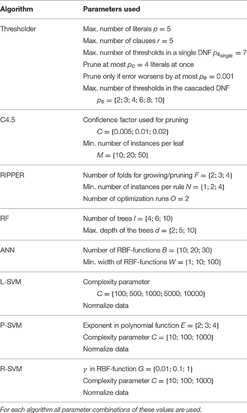
We experimented with different parameter values for the algorithms to find an ideal and fair setting for each of them to represent their performance. This resulted in sets of parameter values where the final setting is selected using a three-fold-cross-validation. For details of the parameter sets see Table 3. Parameters of interpretable models were chosen only based on their performance regardless of model size.

TABLE 3

Table 3. Parameter sets used for the learning algorithms.

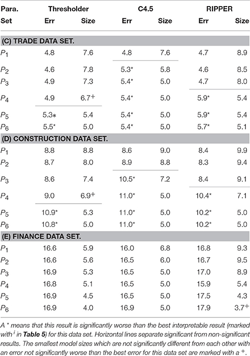
In a second experiment we tried different generalization parameters for all interpretable models of the all-at-once multiclass method. We started with the parameter settings of the previous experiments and changed the values stepwise in a way that the model size of the last parameter combination was five or lower. This is the smallest model size which allows for a separation of three classes. For details see Table 4. That way, we can evaluate a model's performance compared to its size. Lowering the model size is desirable, because a lower model size increases interpretability.

TABLE 4

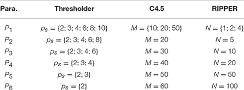
Table 4. The six different generalization parameter sets used for evaluating the correlation between classification error and model size.

A third experiment was performed to study the behavior of IDK-classifications. We tested all algorithms in combination with all multiclass methods supporting IDK-classification, i.e., one-vs-one and one-vs-rest. Additionally, we evaluated Thresholder using different values of τ. Although we tried different values of τ in the training process, τ is always fixed to 0.67 when testing the model. This allows for a proper evaluation. Since we are more interested in the performance using IDK-classifications and model size is of second rank, we use the parameters from Table 3.

5. Results and Discussion

In this section, the results of the three experiments of the case study are shown and discussed. The experiments were performed as described above. Welch's t-test and the Wilcoxon signed-rank test both yielded almost always the same results for our experiments. If they disagreed, result were denoted as significantly different.

In the following tables, the abbreviation err refers to the error rate and size to the model size.

5.1. Performance of All Models and Methods

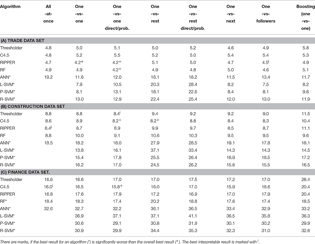
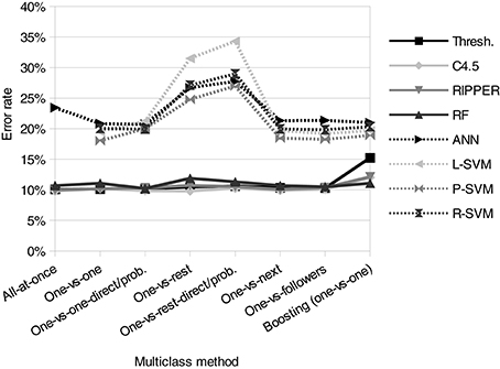
Table 5 shows the error rates for all three data sets, learning algorithms, and multiclass methods. Figure 1 visualizes the mean error rates for the three data sets and shows that all algorithms for interpretable models and RFs perform similarly well and are much better than other algorithms. Different multiclass methods do only affect the performance of the non-thresholds-based algorithms. Boosting does not significantly increase performance. In fact, in most cases it tends to overfit and slightly decreases it.

TABLE 5

Table 5. Error rates of learning algorithms and multiclass methods in percent.

FIGURE 1

Figure 1. Mean error values of learning algorithms and multiclass methods for all data sets.

This experiment shows that interpretable algorithms perform best. Moreover, all of them have a similar classification error. RFs perform slightly worse only for the finance data set. All other non-interpretable algorithms perform significantly worse. Thus, the best performing algorithms are all threshold-based. There is quite a big gap between the error rates of the threshold-based algorithms and the rest, as can be seen in Figure 1. The figure shows that the mean gap over the three data sets is almost always about 10% or higher for each multiclass method which means about twice as many misclassifications. Despite the fact that this figure only plots the mean values for all data sets, it reflects the relative results of each data set as well. Different multiclass methods do not influence the performance of threshold-based algorithms to a great extend. Nevertheless, for ANNs and SVMs, there is a big performance drop when using the one-vs-rest method which was observed in other studies [48, 49, 76] as well. The remaining multiclass methods only show marginal differences among each other. For these data sets, using methods with probability estimates is almost always worse than using methods with simple votes. When ignoring the badly performing one-vs-rest methods, SVMs perform better than ANNs as observed by Kim and Ahn [48]. The simple L-SVMs perform slightly better than the more sophisticated P-SVMs and R-SVMs on the trade and construction data set. The ensemble learning method boosting slightly increases the performance only of some of the bad performing non-interpretable algorithms. However, the best performances are achieved by the threshold-based algorithms and boosting does not increase it. This and the fact that they all perform similarly well leads to the conclusion that the remaining error is noise which can only be eliminated using additional information.

We were surprised at the bad performance of the popular SVMs and ANNs. Therefore, we experimented with different parameters and different kernels in this experiment. Furthermore, we tried a feature selection, but to no avail. There are very few studies comparing these methods with threshold-based models in the field of multiclass credit rating. Furthermore, the credit agencies' processes of determining credit ratings are unknown and differ from agency to agency. We suspect that Creditreform's credit rating is focused on thresholds of account data. Therefore, threshold-based models are more appropriate to reconstruct this credit rating using these data sets. Other approaches from Section 2.2 would probably increase the performance of SVMs and ANNs. However, the small performance gain of methods from these studies compared to the standard algorithms used in this experiment, renders it unlikely to fill the performance gap between the former and the threshold-based algorithms. This applies at least to this problem and these data sets.

5.2. Model Sizes of Interpretable Models

Since all interpretable algorithms yield the best results in the first experiment, we tried to obtain the required model size for this comparable performance. Therefore, we examined performance and model size for different parameters. Figure 2 and Table 6 show the connection of performance and model size when the model size is decreased. They denote statistical significances between error rates and model sizes as well.

FIGURE 2

Figure 2. Error rate and model size for different generalization parameters. A border is plotted between the results which are not significantly worse and the results which are significantly worse than the best result. No border is plotted for the finance data set because there are no results which are significantly worse than the best result.

TABLE 6

Table 6. Error rate in percent and model size for different generalization parameters.

The parameter selection for the previous comparisons is solely based on the classification error and does not consider model size, because we wanted to compare interpretable and non-interpretable algorithms. Therefore, it would be unfair to choose the winner of the similarly performing models solely based on the model size of these experiments. As described above, we did another experiment using different generalization parameters to compare classification error and model size for the all-at-once method of the Thresholder, RIPPER, and C4.5 algorithm. Figure 2 and Table 6 show that increasing the generalization also increases the classification error and lowers the model size at the same time. We consider the smallest model sizes that do not perform significantly worse than the overall best interpretable result of this data set. This is done for each algorithm and data set. In the following, we will refer to these smallest model sizes as the model size of an algorithm. Thus, we can compare the similarly performing algorithms based on their model size.

Furthermore, we did a significance analysis for the model sizes of each algorithm to determine models which are significantly bigger than the smallest model. For the trade data set, Thresholder and C4.5 models are significantly smaller than RIPPER models. Thresholder yields the significantly smallest models for the construction data set as well. For the finance data set the situation is different due to the small amount of low-rated enterprises. Using small models, these enterprises are ignored by the learners which results in model sizes below five. Nevertheless, these model sizes could be achieved without getting significantly worse. For the finance data set, RIPPER models are significantly smaller than Thresholder models. However, the advantage is small and only significant because of the constant model sizes of Thresholder and C4.5 over all repetitions of the experiments. Nevertheless, the mean model size of Thresholder (5.87) is more than one threshold smaller than the sizes of C4.5 (7.13) and RIPPER (6.93). Although the proportions of these numbers might seem small, it has to be taken into consideration that the number of thresholds in these models is much smaller (3.21, 4.13, and 4.33) resulting in differences of about 25%. A reason for the small thresholder models is probably the combination of several multiclass methods and choosing the best ones with the smallest model size. Another reason could be the generalization parameter which directly allows to control the model size.

Figures 3–5 show example models for all interpretable all-at-once algorithms for each data set. For each algorithm and data set we picked a single model out of the 20 repetitions of the parameter set with the biggest generalization that did not perform significantly worse. We took the models whose model sizes were closest to the mean model size for this algorithm, data set, and parameter set. It can be seen that these models are small and only contain a small number of different financial ratios. The finding that few features are sufficient to solve financial problems was shown before [46, 47]. Investigating these models shows that revenue is the most important financial ratio to classify trade and construction enterprises. Despite the fact that revenue is of no importance for financial enterprises, missing values (replaced by zero-values) are indeed a very important discrimination criterion. The worse the enterprise's rating the more missing values seem to appear in their annual accounts. The models catch them by using an upper threshold of or slightly above zero and a second lower threshold of or slightly below zero. All models displayed are of an interpretable structure and of an interpretable size. The size of the Thresholder DNFs is lower than or equal to the size of RIPPER DNFs and DTs. Albeit, DT interpretability is of a different kind.

FIGURE 3

Figure 3. Example models for Thresholder DNFs built on the three data sets. (A) Trade data set model. (B) Construction data set model. (C) Finance data set model.

FIGURE 4

Figure 4. Example models for DTs built on the three data sets. (D) Trade data set model. (E) Construction data set model. (F) Finance data set model.

FIGURE 5

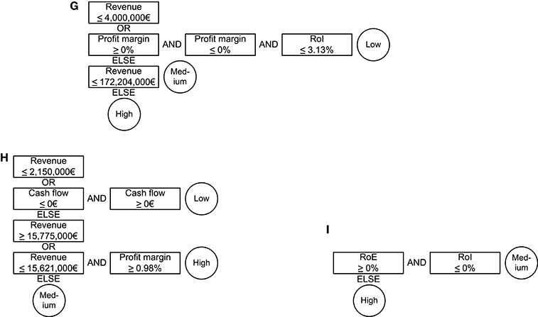
Figure 5. Example models for RIPPER DNFs built on the three data sets. (G) Trade data set model. (H) Construction data set model. (I) Finance data set model.

5.3. Performance of IDK-classifiers

Table 7 shows the results obtained using IDK-classifications. Results which were significantly worse than the best interpretable result (marked with ⁱ in Table 5) or with less than one assigned IDK-label were intentionally left out, because we could not derive benefit from them. The tables show the error rate, the number of IDK-assignments, and die proportion of IDK-assignments per misclassification.

TABLE 7

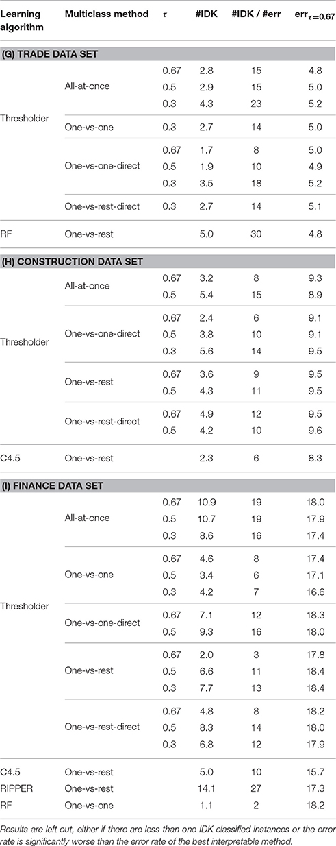
Table 7. Absolute number of IDK-assignments and error rate and number of IDK-assignments per misclassifications in percent of all learning algorithms and IDK-classifier capable multiclass methods.

Roughly a third of the 34 IDK-classifier results assign at least one IDK label and are not significantly worse than the best interpretable result. There are less for the trade (9) and construction data sets (10) and more for the finance data set (17). As expected, increasing the IDK class weight τ leads to a higher amount of IDK-class assignments. In return it leads to higher error rates. However, there are results assigning a higher number of uncertain predictions whose errors are not significantly worse than the error of the best interpretable result.

As mentioned above, the one-vs-rest approach is more likely to produces a tie than the other methods, resulting in more IDK-classifications. However, this does not hold for Thresholder where all methods perform similarly. An explanation for this could be the pruning of the cascaded DNF which might prune the decisions leading to a tie.

There is only a maximum number of five IDK-classifications in the trade and construction data set and 14 in the finance data set which seems to be a very low number compared to the size of a data set. Nevertheless, the purpose of this study is not to find as many IDK-instances as possible. Correct predictions are still the most important observations. However, it is desirable to turn as many misclassifications as possible into IDK-classifications. Consider that these absolute numbers of IDK-classifications are only observed on the test data set which is 33% of the whole data. Comparing their amount with the number of misclassifications yields rates of 15 to 30% IDK-classifications per misclassification without worsening the accuracy significantly.

While performing not significantly different, RFs yield the most IDK-classifications for the trade data set, Thresholder for the construction data set, and RIPPER for the finance data set. However, only Thresholder yields interpretable models to explain these IDK-assignments. Figure 6 shows example DNFs built by Thresholder using IDK-classification. For each data set we selected the setting which yields the most IDK-assignments without performing significantly worse than the best interpretable result. The model whose number of IDK-assignments is closest to the mean number of IDK-assignments for this data set and settings is displayed. The trade and finance models are similar to those in Figure 3, but with one additional threshold which discriminates the IDK-label from the rest. The model built on the construction data set is much bigger. An explanation can be found in the missing optimization of the model size as done in the experiment above. However, we think that these models are well suited for decision support with their additional information about doubt.

FIGURE 6

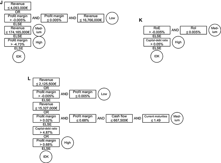
Figure 6. Example models for Thresholder DNFs using IDK-classifications built on the three data sets. (J) Trade data set model. (K) Finance data set model. (L) Construction data set model.

6. Conclusions

Even though the results are empirical, we conclude that interpretable models are well suited for classification problems in finance. Those performed slightly better than non-interpretable models in a prior study on insolvency prediction [3]. In this study on credit rating interpretable models even outperformed non-interpretable models reducing the misclassifications by about 50%. The results can be explained by the way classification is achieved. Insolvency happens when an enterprise cannot pay its debts which is caused by several financial factors in contrast to credit ratings which are at least partially man-made classifications. We conclude that man-made classifications are based on few thresholds, and therefore, can be detected by threshold-based algorithms. ANNs and SVMs might build models which are too complex for these simple rules and lead to an overfitting of the data. The fact that less sophisticated L-SVMs outperform P-SVMs and R-SVMs on two data sets confirms this assumption. Furthermore, boosting which reduces bias by building more complex models does not increase the performance. Since all threshold-based methods perform similarly, we expect the remaining error to be noise which cannot be explained by the data. In fact, Creditreform gave information that annual accounts only influence their rating by 20%. Instead, qualitative factors like payment experiences from the past are more important.

There are three main contributions of this paper. We showed that threshold-based methods and interpretable methods outperformed other methods like ANNs and SVMs in a case study on credit rating. The second contribution is a new interpretable multiclass method to learn DNFs by adopting several well known multiclass methods. The classification error of this method is similar to the other interpretable methods, but further experiments show smaller model sizes with similar error rates. As a third contribution, we introduce an interpretable method to express doubt in the classification. These IDK-labels can be used as a marker for doubtful classifications. These marks allow for a selective application of more expensive classification methods, e.g., classification by hand. However, simple methods can still be applied, e.g., assigning the most critical label or randomly choosing a label.

Practical implications of our work are that interpretable models are well suited for some classification problems in finance. Despite the fact that all interpretable models have a comparable classification error, we recommend using our Thresholder algorithm because it offers some benefits. Thresholder builds the smallest models, it allows to adjust the amount of interpretability by determining a maximum model size, it offers the highest amount of IDK-assignments per misclassifications, and it is the only algorithm that offers interpretable models for IDK-assignments.

As future work, we would like to implement the generalization of our multiclass method to work for more than three classes and evaluate it accordingly. These models will get much bigger due to logical operations on more DNFs. Experiments will show whether the resulting cascaded DNFs can be pruned down to an interpretable size. Furthermore, we would like to identify additional problem statements where interpretable models are non-inferior to interpretable models. We suggest using sophisticated models only when it is necessary. However, to determine this necessity it is important to understand which problems are solvable by interpretable models.

Author Contributions

LO developed the algorithm Thresholder together with SW. LO implemented the algorithms and conducted and evaluated the tests. The manuscript was drafted by LO and reworked by LO and SW together. All authors read and approved the final manuscript.

Conflict of Interest Statement

The authors declare that the research was conducted in the absence of any commercial or financial relationships that could be construed as a potential conflict of interest.

The reviewer JP and handling Editor declared their shared affiliation, and the handling Editor states that the process nevertheless met the standards of a fair and objective review.

Acknowledgments

We acknowledge support by the German Research Foundation and the Open Access Publication Funds of the Göttingen University. Furthermore, this research paper includes large parts of the Ph.D. thesis of Obermann [77].

Footnotes

1. ^Enterprise size is a feature in the database and its calculation is undocumented.

2. ^Technically they use the number of rules multiplied by the mean rule size.

References

1. Kainulainen L, Miche Y, Eirola E, Yu Q, Frénay B, Séverin E, et al. Ensembles of local linear models for bankruptcy analysis and prediction. Case Stud Business Indust Govern Stat. (2014) 4:116–33.

Google Scholar

2. Florez-Lopez R, Ramon-Jeronimo JM. Enhancing accuracy and interpretability of ensemble strategies in credit risk assessment. A correlated-adjusted decision forest proposal. Exp Syst Appl. (2015) 42:5737–53. doi: 10.1016/j.eswa.2015.02.042

CrossRef Full Text | Google Scholar

3. Obermann L, Waack S. Demonstrating non-inferiority of easy interpretable methods for insolvency prediction. Exp Syst Appl. (2015) 42:9117–28. doi: 10.1016/j.eswa.2015.08.009

CrossRef Full Text | Google Scholar

4. Tomczak JM, Zieba M. Classification Restricted Boltzmann Machine for comprehensible credit scoring model. Exp Syst Appl. (2015) 42:1789–96. doi: 10.1016/j.eswa.2014.10.016

CrossRef Full Text | Google Scholar

5. Hand DJ. Classifier technology and the illusion of progress. Stat Sci. (2006) 21:1–14. doi: 10.1214/088342306000000060

CrossRef Full Text | Google Scholar

6. Crook JN, Edelman DB, Thomas LC. Recent developments in consumer credit risk assessment. Eur J Oper Res. (2007) 183:1447–65. doi: 10.1016/j.ejor.2006.09.100

CrossRef Full Text | Google Scholar

7. Sun J, Li H, Huang QH, He KY. Predicting financial distress and corporate failure: a review from the state-of-the-art definitions, modeling, sampling, and featuring approaches. Knowl Based Syst. (2014) 57:41–56. doi: 10.1016/j.knosys.2013.12.006

CrossRef Full Text | Google Scholar

8. Finlay S. Multiple classifier architectures and their application to credit risk assessment. Eur J Oper Res. (2011) 210:368–78. doi: 10.1016/j.ejor.2010.09.029

CrossRef Full Text | Google Scholar

9. Angilella S, Mazzù S. The financing of innovative SMEs: a multicriteria credit rating model. Eur J Oper Res. (2015) 244:540–54. doi: 10.1016/j.ejor.2015.01.033

CrossRef Full Text | Google Scholar

10. Beaver WH. Financial ratios as predictors of failure. J Account Res. (1966) 4:71–111. doi: 10.2307/2490171

CrossRef Full Text | Google Scholar

11. Altman EI. Financial ratios, discriminant analysis and the prediction of corporate bankruptcy. J Finance (1968) 23:589–609. doi: 10.1111/j.1540-6261.1968.tb00843.x

CrossRef Full Text | Google Scholar

12. Blum M. Failing company discriminant analysis. J Account Res. (1974) 12:1–25. doi: 10.2307/2490525

CrossRef Full Text | Google Scholar

13. Laitinen EK. Prediction of failure of a newly founded firm. J Business Ventur. (1992) 7:323–40. doi: 10.1016/0883-9026(92)90005-C

CrossRef Full Text | Google Scholar

14. Martin D. Early warning of bank failure: a logit regression approach. J Bank Finan. (1977) 1:249–76. doi: 10.1016/0378-4266(77)90022-X

CrossRef Full Text

15. Ohlson, JA. Financial ratios and the probabilistic prediction of bankruptcy. J Account Res. (1980) 18:109–31. doi: 10.2307/2490395

CrossRef Full Text | Google Scholar

16. Gentry JA, Newbold P, Whitford DT. Classifying bankrupt firms with funds flow components. J Account Res. (1985) 23:146–60. doi: 10.2307/2490911

CrossRef Full Text | Google Scholar

17. Zmijewski ME. Methodological issues related to the estimation of financial distress prediction models. J Account Res. (1984) 22:59–82. doi: 10.2307/2490859

CrossRef Full Text | Google Scholar

18. Skogsvik K. Current cost accounting ratios as predictors of business failure: the Swedish case. J Business Finan Account. (1990) 17:137–60. doi: 10.1111/j.1468-5957.1990.tb00554.x

CrossRef Full Text | Google Scholar

19. Tam KY, Kiang MY. Managerial applications of neural networks: the case of bank failure predictions. Manage Sci. (1992) 38:926–47. doi: 10.1287/mnsc.38.7.926

CrossRef Full Text | Google Scholar

20. Wilson RL, Sharda R. Bankruptcy prediction using neural networks. Decis Supp Syst. (1994) 11:545–57. doi: 10.1016/0167-9236(94)90024-8

CrossRef Full Text

21. Charitou A, Neophytou E, Charalambous C. Predicting corporate failure: empirical evidence for the UK. Eur Account Rev. (2004) 13:465–97. doi: 10.1080/0963818042000216811

CrossRef Full Text | Google Scholar

22. Neves JC, Vieira A. Improving bankruptcy prediction with hidden layer learning vector quantization. Eur Account Rev. (2006) 15:253–71. doi: 10.1080/09638180600555016

CrossRef Full Text | Google Scholar

23. Fan A, Palaniswami M. Selecting bankruptcy predictors using a support vector machine approach. In: Proceedings of the International Joint Conference on Neural Networks, Vol. 6 (2000). p. 354–9. doi: 10.1109/ijcnn.2000.859421

CrossRef Full Text | Google Scholar

24. Härdle W, Lee YJ, Schäfer D, Yeh YR. Variable selection and oversampling in the use of smooth support vector machines for predicting the default risk of companies. J Forecast. (2009) 28:512–34. doi: 10.1002/for.1109

CrossRef Full Text | Google Scholar

25. Harris T. Credit scoring using the clustered support vector machine. Exp Syst Appl. (2015) 42:741–50. doi: 10.1016/j.eswa.2014.08.029

CrossRef Full Text | Google Scholar

26. Danenas P, Garsva G. Selection of support vector machines based classifiers for credit risk domain. Exp Syst Appl. (2015) 42:3194–204. doi: 10.1016/j.eswa.2014.12.001

CrossRef Full Text | Google Scholar

27. Frydman H, Altman EI, li Kao D. Introducing recursive partitioning for financial classification: the case of financial distress. J Finan. (1985) 40:269–91. doi: 10.1111/j.1540-6261.1985.tb04949.x

CrossRef Full Text | Google Scholar

28. Fernández E, Olmeda I. Bankruptcy prediction with artificial neural networks. In: Mira J, Sandoval F, editors. From Natural to Artificial Neural Computation. Vol. 930 of Lecture Notes in Computer Science. Berlin; Heidelberg: Springer (1995). p. 1142–6.

29. Fritz S, Hosemann D. Restructuring the credit process: behaviour scoring for German corporates. Int J Intell Syst Account Finan Manage. (2000) 9:9–21. doi: 10.1002/(SICI)1099-1174(200003)9:1<9::AID-ISAF168>3.0.CO;2-Q

CrossRef Full Text | Google Scholar

30. Slowinski R, Zopounidis C. Application of the rough set approach to evaluation of bankruptcy risk. Intell Syst Account Finan Manage. (1995) 4:27–41. doi: 10.1002/j.1099-1174.1995.tb00078.x

CrossRef Full Text | Google Scholar

31. McKee TE. Developing a bankruptcy prediction model via rough sets theory. Int J Intell Syst Account Finance Manag. (2000) 9:159–73. doi: 10.1002/1099-1174(200009)9:3<159::AID-ISAF184>3.0.CO;2-C

CrossRef Full Text | Google Scholar

32. Bose I. Deciding the financial health of dot-coms using rough sets. Inform Manage. (2006) 43:835–46. doi: 10.1016/j.im.2006.08.001

CrossRef Full Text | Google Scholar

33. Kotsiantis S, Tzelepis D, Koumanakos E, Tampakas V. Efficiency of machine learning techniques in bankruptcy prediction. In: 2nd International Conference on Enterprise Systems and Accounting. Thessaloniki (2005).

34. Brodag T. PAC-Lernen zur Insolvenzerkennung und Hotspot-Identifikation: Anwendung Statistischer Modelle des Algorithmischen Lernens auf Betriebswirtschaftliche und Bioinformatische Probleme der Praxis. Göttingen: University of Göttingen (2008).

35. Kwak W, Shi Y, Kou G. Predicting bankruptcy after The Sarbanes-Oxley act using the most current data mining approaches. J Business Econ Res. (2012) 10:233–42. doi: 10.19030/jber.v10i4.6899

CrossRef Full Text | Google Scholar

36. Alfaro Cortés E, Gámez Martínez M, García Rubio N. Multiclass corporate failure prediction by adaboost.M1. Int Adv Econ Res. (2007) 13:301–12. doi: 10.1007/s11294-007-9090-2

CrossRef Full Text

37. Alfaro E, García N, Gámez M, Elizondo D. Bankruptcy forecasting: an empirical comparison of AdaBoost and neural networks. Decis Supp Syst. (2008) 45:110–22. doi: 10.1016/j.dss.2007.12.002

CrossRef Full Text | Google Scholar

38. Nanni L, Lumini A. An experimental comparison of ensemble of classifiers for bankruptcy prediction and credit scoring. Exp Syst Appl. (2009) 36(Pt 2):3028–33. doi: 10.1016/j.eswa.2008.01.018

CrossRef Full Text | Google Scholar

39. Kang DK, Kim MJ. Performance enhancement of SVM ensembles using genetic algorithms in bankruptcy prediction. In: Proceedings of the 3rd International Conference on Advanced Computer Theory and Engineering (ICACTE '10), Vol. 2 (2010). p. V2154–8.

Google Scholar

40. Abellán J, Mantas CJ. Improving experimental studies about ensembles of classifiers for bankruptcy prediction and credit scoring. Exp Syst Appl. (2014) 41:3825–30. doi: 10.1016/j.eswa.2013.12.003

CrossRef Full Text | Google Scholar

41. Wang G, Ma J, Yang S. An improved boosting based on feature selection for corporate bankruptcy prediction. Exp Syst Appl. (2014) 41:2353–61. doi: 10.1016/j.eswa.2013.09.033

CrossRef Full Text | Google Scholar

42. Balcaen S, Ooghe H. 35 years of studies on business failure: an overview of the classic statistical methodologies and their related problems. Brit Account Rev. (2006) 38:63–93. doi: 10.1016/j.bar.2005.09.001

CrossRef Full Text | Google Scholar

43. Dimitras AI, Zanakis SH, Zopounidis C. A survey of business failures with an emphasis on prediction methods and industrial applications. Eur J Oper Res. (1996) 90:487–513. doi: 10.1016/0377-2217(95)00070-4

CrossRef Full Text | Google Scholar

44. Verikas A, Kalsyte Z, Bacauskiene M, Gelzinis A. Hybrid and ensemble-based soft computing techniques in bankruptcy prediction: a survey. Soft Comput. (2010) 14:995–1010. doi: 10.1007/s00500-009-0490-5

CrossRef Full Text | Google Scholar

45. Huang Z, Chen H, Hsu CJ, Chen WH, Wu S. Credit rating analysis with support vector machines and neural networks: a market comparative study. Decis Supp Syst. (2004) 37:543–58. doi: 10.1016/S0167-9236(03)00086-1

CrossRef Full Text | Google Scholar

46. Cao L, Guan LK, Jingqing Z. Bond rating using support vector machine. Intell Data Anal. (2006) 10:285–96.

Google Scholar

47. Hájek P. Municipal credit rating modelling by neural networks. Decis Supp Syst. (2011) 51:108–18. doi: 10.1016/j.dss.2010.11.033

CrossRef Full Text | Google Scholar

48. Kim Kj, Ahn H. A corporate credit rating model using multi-class support vector machines with an ordinal pairwise partitioning approach. Comput Oper Res. (2012) 39:1800–11. doi: 10.1016/j.cor.2011.06.023

CrossRef Full Text

49. Guo X, Zhu Z, Shi J. A corporate credit rating model using support vector domain combined with fuzzy clustering algorithm. Math Prob Eng. (2012) 2012:302624. doi: 10.1155/2012/302624

CrossRef Full Text | Google Scholar

50. Kwon J, Choi K, Suh Y. Double ensemble approaches to predicting firms' credit rating. In: PACIS. Jeju Island (2013). p. 158.

51. Craven MW, Shavlik JW. Extracting tree-structured representations of trained networks. Adv Neural Inform Process Syst. (1996) 8:24–30.

Google Scholar

52. Jang JSR, Sun CT. Functional equivalence between radial basis function networks and fuzzy inference systems. IEEE Trans Neural Netw. (1993) 4:156–9. doi: 10.1109/72.182710

PubMed Abstract | CrossRef Full Text | Google Scholar

53. Mantas CJ, Puche JM, Mantas JM. Extraction of similarity based fuzzy rules from artificial neural networks. Int J Approx Reason. (2006) 43:202–21. doi: 10.1016/j.ijar.2006.04.003

CrossRef Full Text | Google Scholar

54. Féraud R, Clérot F. A methodology to explain neural network classification. Neural Netw. (2002) 15:237–46. doi: 10.1016/S0893-6080(01)00127-7

PubMed Abstract | CrossRef Full Text | Google Scholar

55. Johansson U, König R, Niklasson L. The truth is in there-rule extraction from opaque models using genetic programming. In: FLAIRS Conference. Miami Beach, FL (2004). p. 658–63.

56. Barbella D, Benzaid S, Christensen JM, Jackson B, Qin XV, Musicant DR. Understanding support vector machine classifications via a recommender system-like approach. In: DMIN. Las Vegas, NV (2009). p. 305–11.

Google Scholar

57. Martens D, Baesens B, Gestel TV, Vanthienen J. Comprehensible credit scoring models using rule extraction from support vector machines. Eur J Oper Res. (2007) 183:1466–76. doi: 10.1016/j.ejor.2006.04.051

CrossRef Full Text | Google Scholar

58. Su CT, Chen YC. Rule extraction algorithm from support vector machines and its application to credit screening. Soft Comput. (2011) 16:645–58. doi: 10.1007/s00500-011-0762-8

CrossRef Full Text | Google Scholar

59. Kim JW, Weistroffer HR, Redmond RT. Expert systems for bond rating: a comparative analysis of statistical, rule-based and neural network systems. Exp Syst. (1993) 10:167–72. doi: 10.1111/j.1468-0394.1993.tb00093.x

CrossRef Full Text | Google Scholar

60. Jones S, Johnstone D, Wilson R. An empirical evaluation of the performance of binary classifiers in the prediction of credit ratings changes. J Bank Finan. (2015) 56:72–85. doi: 10.1016/j.jbankfin.2015.02.006

CrossRef Full Text | Google Scholar

61. Virág M, Nyitrai T. Is there a trade-off between the predictive power and the interpretability of bankruptcy models? The case of the first Hungarian bankruptcy prediction model. Acta Oeconom. (2014) 64:419–40. doi: 10.1556/AOecon.64.2014.4.2

CrossRef Full Text

62. Hall M, Frank E, Holmes G, Pfahringer B, Reutemann P, Witten IH. The WEKA data mining software: an update. SIGKDD Explor. (2009) 11:10–8. doi: 10.1145/1656274.1656278

CrossRef Full Text | Google Scholar

63. Fürnkranz J, Widmer G. Incremental reduced error pruning. In: International Conference on Machine Learning. New Brunswick, NJ (1994).

64. Cohen W. Fast effective rule induction. In: Twelfth International Conference on Machine Learning. Tahoe City, CA (1995). doi: 10.1016/b978-1-55860-377-6.50023-2

PubMed Abstract | CrossRef Full Text | Google Scholar

65. Rissanen J. Modeling by shortest data description. Automatica (1978) 14:465–71. doi: 10.1016/0005-1098(78)90005-5

CrossRef Full Text | Google Scholar

66. Quinlan JR. C4.5: Programs for Machine Learning. Morgan Kaufmann (1993). Available online at: http://books.google.de/books?id=HExncpjbYroC

67. Quinlan JR. Induction of decision trees. Mach Learn. (1986) 1:81–106. doi: 10.1007/BF00116251

CrossRef Full Text

68. Friedman J. Another Approach to Polychotomous Classification. Stanford, CA: Department of Statistics, Stanford University (1996).

69. Kreßel UHG. Pairwise classification and support vector machines. In: Schölkopf B, Burges CJC, Smola AJ editors, Advances in Kernel Methods: Support Vector Learning. Cambridge, MA: MIT Press (1999). p. 255–68.

PubMed Abstract

70. Kwon YS, Han I, Lee KC. Ordinal pairwise partitioning (OPP) approach to neural networks training in bond rating. Int J Intell Syst Account Finan Manage. (1997) 6:23–40. doi: 10.1002/(SICI)1099-1174(199703)6:1<23::AID-ISAF113>3.0.CO;2-4

CrossRef Full Text | Google Scholar

71. Verband der Vereine Creditreform e V. DAFNE Database. (2015). Available online at: http://en.creditreform.de/portfolio/marketing-services/target-group-analysis.html (Accessed August 17, 2016).

72. Welch BL. The generalization of 'student's' problem when several different population variances are involved. Biometrika (1947) 34:28–35. doi: 10.2307/2332510

CrossRef Full Text | Google Scholar

73. Wilcoxon F. Individual comparisons by ranking methods. Biometrics (1945) 1:80–3. doi: 10.2307/3001968

CrossRef Full Text | Google Scholar

74. Alpaydin E. Introduction to Machine Learning. Adaptive computation and machine learning. MIT Press (2004). Available online at: https://books.google.de/books?id=1k0_-WroiqEC

75. García S, Fernández A, Luengo J, Herrera F. A study of statistical techniques and performance measures for genetics-based machine learning: accuracy and interpretability. Soft Comput. (2009) 13:959–77. doi: 10.1007/s00500-008-0392-y

CrossRef Full Text | Google Scholar

76. Hsu CW, Lin CJ. A comparison of methods for multiclass support vector machines. IEEE Trans Neural Netw. (2002) 13:415–25. doi: 10.1109/72.991427

PubMed Abstract | CrossRef Full Text | Google Scholar

77. Obermann L. Interpretable Binary and Multiclass Prediction Models for Insolvencies and Credit Ratings. University of Göttingen (2016). Available online at: http://hdl.handle.net/11858/00-1735-0000-0028-8779-4