A 3D ray-tracing based model for radiowave simulations in vegetated environments with wind-induced dynamics

Introduction: This paper proposes an extension of a ray-tracing based model for radiowave propagation in the presence of vegetation, to account for the wind-induced channel dynamics in vegetated environments. The original propagation model uses various point scatterers with specific re-radiation and it has been proven to be suitable for a wide range of scenarios. However, the swaying motion of the tree branches and leaves, as an effect of the wind, creates a constantly changing environment that influences the propagating radio signals in both amplitude and phase, resulting in signal level fluctuations.

Methods: A large measurement campaign intending to record and characterize the effect of wind-induced dynamics in vegetated environments, was conducted in a controlled environment, inside an anechoic chamber. Experiments included various wind directions and at varying speeds: stationary (0 m/s), low (1.9 m/s) and high (4.7 m/s). The dynamic re-radiation pattern of trees present in the radio path were recorded at 20 and 62.4 GHz signal frequencies. The available experimental data was then used to develop a statistical model which is sought to characterize wind-induced dynamics of the point scatterers’ re-radiation function. Finally, the performance of the proposed dynamic model while predicting the received signal level fluctuations inside a tree formation scenario, was assessed against dynamic directional spectra measurements conducted in a controlled environment, for four different artificially generated wind incidences and two wind speeds, low (1.9 m/s) and high (4.7 m/s).

Results and discussion: This experiment proved that the proposed elementary model could be an asset on the characterization of the time-varying effects found in vegetation areas under wind influence.

1 Introduction

The presence of trees and vegetation areas will substantially degrade radio communication system performance, causing signal attenuation (absorption), scattering, and (de)polarization (Caldeirinha, 2001). Additionally, the swaying motion of the branches and leaves as an effect of the wind, creates a constantly changing environment that influences the propagating radio signals in both amplitude and phase, resulting in small-scale signal fluctuations. These phenomena become particularly critical at higher frequencies, in which the size of leaves and smaller branches present in the canopy, becomes comparable to the propagating signal wavelength (Rogers and et al., 2002).

In recent decades, several models addressing the propagation phenomena in the presence of trees and vegetation volumes have been proposed in the literature. One of the common modelling approaches is the empirical modelling. Empirical models (Weissberger, 1982; International Radio Consultative Committee, 1986; COST235, 1995; Meng et al., 2009; Seville and Craig, 1995), which are based on simple equations and developed based on specific on-site measurements, have successfully been used to characterise the well-known “dual-slope” attenuation effect in various scenarios and frequency bands. Nevertheless, due to their site-specific nature, they usually lack of accuracy outside the model scope and, in general, these models do not account for time-variant channel properties due to wind induced dynamics.

On the other hand, full wave theoretical models using deterministic approaches (Torrico et al., 1998; Torrico and Lang, 2012; Chee et al., 2013; Wang and Sarabandi, 2005; Wang, 2006) are able to provide very reliable propagation phenomena predictions in a wide range of vegetated environments. However, such models are often very complex in nature, requiring numerical approximations to provide accurate solutions, and its true applicability in real scenarios might be difficult, since this modelling approach requires an accurate electromagnetic description of the tree geometry, including parameters such as, leaf density, area, orientation and thickness, which are prohibitively time-consuming to obtain in a real-sized forests (Wang, 2006). This time-consumption problem quickly escalates whenever the wind-induced time-variability of the radio channel is to be considered, since a huge amount of simulations would be required as well as the respective time-variant input parameter extraction.

The Radiative Energy Transfer (RET) and discrete RET (dRET) based models have also been successfully used to characterise the propagation phenomena in the presence of vegetation. Indeed, several studies presented in (Fernandes, 2007; Fernandes et al., 2005; Caldeirinha et al., 2010)used the transfer theory to predict, not only the excess attenuation caused by the presence of vegetation volumes, but also the directional spectra inside various tree formations in both in- and outdoor environments. Additionally, early work aiming at the extension of the dRET model to account for the wind-induced channel dynamics has been proposed in (Morgadinho et al., 2012), in which a Multistate Markov model was used to provide small-scale signal fluctuation. However, the applicability of the transfer theory in forest environments, seems also to be limited. On one hand, the homogeneous medium consideration given in the original RET model (Johnson and Schwering, 1985) clashes with real forests, which usually exhibit free space gaps between adjacent trees. On the other hand, the discretized RET model (Didascalou et al., 2000), had overcome the homogeneous limitation of the original transfer theory but, since it requires the discretization of the vegetation volumes into small cells, it might become numerically intractable for large propagation distances (Wang and Sarabandi, 2007).

The point scatterer formulation based model is another modelling approach for radiowave propagation in vegetation, in which point scatterers are distributed within the computational volume to characterise the trees’ impact on the radiowave signal propagation. The referred modelling approach has been successively developed, extended and extensively validated in a wide range of scenarios, including various indoor tree formation scenarios with some degree of inhomogeneity within the vegetation volume (Leonor et al., 2014; Leonor et al., 2017); outdoor line-of-trees scenarios, including both in- and out-of-leaf foliation states and inhomogeneous outdoor tree formations with mixed species (Leonor et al., 2018); and indoor tree formation scenarios with oblique/slant incidence, i.e., three-dimension (3D) scenarios (Leonor et al., 2019). However, to the best of the authors’ knowledge, the effect of the wind, and the consequent signal level fluctuations over time, has not yet been accounted in this modelling approach. To this extent, this paper aims at the extension of the point scatterer formulation into a doubly-selective model for propagation in vegetation (Leonor, 2018).

The paper is then organised as follows. In Section 2, a brief overview of the point scatterer formulation modelling approach is presented. Section 3 aims at the characterisation of the effect of wind-induced dynamics on the received signal level. To this extent, measurements intending to record the dynamic re-radiation function of a tree specimen, were conducted in a controlled environment, inside a anechoic chamber, with artificially generated wind from various directions and speeds. Subsequently, the available experimental data and its statistical analysis was used to develop an elementary dynamic model characterising the radiowave propagation phenomena of a tree under wind influence. This dynamic elementary model was developed in two different stages. In the first stage, time-variant input propagation parameters were extracted directly from dynamic re-radiation measurements, yielding to a very reliable description of the signal level variations, specially in the forward scattering direction. However, its application to tree formation scenarios is cumbersome due to the synchronous nature of the input propagation parameters extraction method. To this extend a second dynamic model, based on well-known statistical distributions was proposed. Despite some limitations identified in this second method, it enabled the modelling approach to be applicable in complex vegetation structures, such as tree formations. The assessment of the statistical based dynamic model while predicting the received signal level fluctuations in a tree formation scenario is presented in Section 4. The performance of the proposed doubly-selective model was assessed against dynamic directional spectra measurements conducted inside an anechoic chamber, for four different artificially generated wind incidences and two wind speeds. Finally, Section 5, addresses some conclusions and raises directions for further work.

2 Original model overview

The ray-tracing based model proposed in (Leonor et al., 2014), and latter enhanced in Leonor et al. (2018) and in Leonor et al. (2019), uses point scatterer formulation to characterize the radiowave propagation phenomena of trees. In this model, trees present in the simulation radio channel are characterized using a set of point scatterers, which are distributed in various circles with varying heights and widths, providing a relatively homogeneous point scatterer distribution across the vegetation volume. A detailed description on algorithm defined for the point scatterer distribution, which will generate sort of a sphere which dimensions are dependent on the canopy height and width, can be found in Leonor et al. (2019). Figure 1 depicts an example of a small tree modelled using the point scatterer distribution.

Figure 1

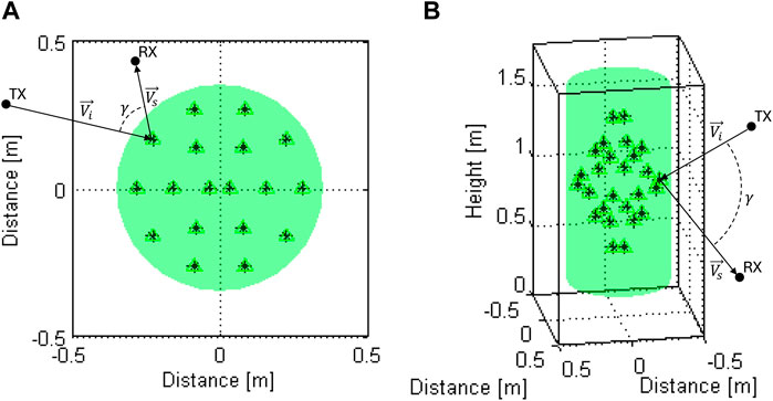
Figure 1. 3D tree physical model: (A) Top and (B) Rotation view.

To gather the interactions between all point scatterers present in the simulation volume a two-iteration ray-tracing algorithm is used. The first iteration of ray launching includes the direct component and also the rays travelling from the transmitter (TX) toward the scattered points and bounced back to the receiver (RX). In the second iteration, point scatterers illuminated with the rays of first iteration are assumed as new TXs, and the rays travelling from each point toward the other scatterers and subsequently bounced to the RX are included. Finally, the received signal complex envelope is calculated by coherently adding all the multipath components arriving at the receiving antenna, for each time-step.

Each tree, and its respective point scatterers, is characterized by a set of input propagation parameters, which includes.

• ${\beta }_i$, that regulates the forward lobe beamwidth of the point scatterers’ re-radiation pattern;

• $k_i$, used to manage the amount of excess loss suffered by the radiowave rays travelling through the tree volume.

The point scatterers’ re-radiation function is based on the normalized version of the well-known phase function model, originally presented in Ulaby et al. (1990), which is expressed by

$\rho \left(\gamma \right)=\frac{\alpha {\left(\frac{2}{\beta }\right)}^2{e}^{-{\left(\frac{\gamma }{\beta }\right)}^2}+\left(1-\alpha \right)}{\alpha {\left(\frac{2}{\beta }\right)}^2+\left(1-\alpha \right)}(1)$

where $\gamma$ is the angular difference (in radians), between the incident and scattered rays, $\alpha$ controls the level of the scattered power and $\beta$ is the forward lobe beamwidth. It was found in Leonor et al. (2014) that successively applying the phase function for different values of $\alpha$ and $\beta$ to the tree physical model, along with the $k$ parameter used to manage the excess loss of the ray travelling inside the vegetation volume, the $\beta$ parameter alone was suitable to characterise the shape of the tree re-radiation function. Hence, to simplify the propagation model and the number of its input propagation parameters, the $\alpha$ was fixed at half-scale (0.5).

Equation 1 is derived for two-dimension (2D) scenarios, however, based on the measurement results presented in Leonor et al. (2019), it was concluded that the symmetry around the forward scattering direction is found, not only in the azimuth plane, but also in the elevation plane. Therefore, to characterize the tree scattering phenomena in 3D scenarios, the $\gamma$ parameter was defined as the angle between the 3D vectors representing the incidence and the scattering directions, $\overrightarrow{V_i}$ and $\overrightarrow{V_s}$, respectively, given by Equation 2

$\gamma =\arccos \left(\frac{\overrightarrow{V_i}\cdot \overrightarrow{V_s}}{\left|\overrightarrow{V_i}\right|\left|\overrightarrow{V_s}\right|}\right).(2)$

Additionally, rays travelling through the vegetation volume will account for excess attenuation. Considering a generic scenario composed by $N_T$ trees, as depicted in Figure 2, the total excess loss $L_{E{x}_{\mathit{total}}}$ of the rays travelling inside the vegetation volume, is given in dB, by Equation 3

$L_{E{x}_{\mathit{total}}}={\displaystyle \sum _{i=1}^N}{k}_i{\left(d_i-d_{i-1}\right)}^{0.5}\left[dB\right](3)$

where, $N_T$ is the number of the trees intersected, $d_i$ is the total transmission distance inside the $i^{th}$ tree, as depicted in Figure 2, and $k_i$ is an input parameter used to characterize the attenuation slope of the specific $i^{th}$ tree (Leonor et al., 2018).

Figure 2

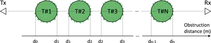
Figure 2. Generic simulation scenario.

As far as input propagation parameter extraction is concerned, an empirical method was proposed in (Leonor et al. (2018)), which is based on two simple measurements that can be relatively easily conducted in an outdoor forest environment. The aim of such measurements, which are to be taken with the RX at positions $\varphi =0°$ and $\varphi =\pm 90°$ (see Figure 5), is to evaluate the tree insertion loss $(I_L)$ and the tree front-to-side signal discrimination $(G_{FS})$, i.e., the difference between the signal level recorded at the forward and the side scattering directions, respectively. Both $I_L$ and $G_{FS}$ values are given in decibel units (dB). After the proper characterization of $I_L$ and $G_{FS}$ parameters, ${\beta }_i$ and $k_i$ values can be extracted using,

${\beta }_{\mathit{emp}}=40e^{-0.02G_{FS}}\left[°\right](4)$

and

$k_{\mathit{emp}}=8{\left(\frac{I_L}{T_d}\right)}^{0.2}\left[dB/m\right](5)$

where $I_L$ is the tree insertion loss and $T_d$ the tree diameter.

3 Measurement system overview

Measurements intending to record time-varying received signal level, caused by the swaying motion of the tree branches, twigs and leafs, were carried out at 20 and 62.4 GHz.

The 20 GHz measurement system, depicted in Figure 3 a through block diagram, consists of a Gunn diode voltage controlled oscillator (VCO), providing a continuous-wave (CW) tone of 20 GHz rated at 20 dB m, which is radiated to the radio path using a 10 dBi standard horn antenna with a half-power beamwidth (HPBW) of approximately $45°$. At the RX side, the radio-frequency (RF) signal was acquired by a 20 dBi standard gain horn antenna with a HPBW of approximately $17°$. The received signal travelled to a frequency down conversion section through a waveguide attenuator, which includes a variable attenuator (Att) to enhance the system dynamic range, a balanced mixer and a 19.78 GHz local oscillator (LO). The LO is used to down-convert the RF signal into a 220 MHz intermediate-frequency (IF) signal which is subsequently amplified by a 44 dB low noise amplifier (LNA). At the data logger section the IF signal was acquired by logarithmic amplifier (LogAmp) and a data acquisition (DAQ) card, enabling fast signal acquisition, up to 100 ksamp/s.

Figure 3

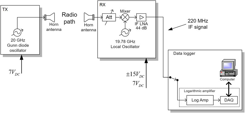
Figure 3. 20 GHz measurement system block diagram.

The 62.4 GHz measurement system was built using a phase locked loop oscillator (PLO) composed by a Gunn diode oscillator tuned at 20.8 GHz and a frequency multiplier used to triple the signal frequency. The ensemble oscillator-multiplier generates a RF signal tuned at 62.4 GHz and rated at 16 dB m. This RF signal is transmitted to the radio path over a waveguide attenuator and a 25 dBi standard horn antenna with a HPBW of approximately $9°$. The block diagram of the millimetre-wave (mmWave) measurement system is depicted in Figure 4.

Figure 4

Figure 4. 62.4 GHz measurement system block diagram.

At the RX end, a similar 25 dBi standard horn antenna was used to acquire the RF signal, which in turn, was transmitted to a frequency down-conversion set, using a waveguide attenuator. The frequency conversion stage consists of a balanced mixer and a VCO operating and 61.8 GHz, which converts the RF signal into a 600 MHz IF signal. The IF component is then amplified by a 44 dB LNA and filtered by a band-pass filter (BPF) centred at 600 MHz with a 5.38 MHz of bandwidth (−3 dB). Similarly to the 20 GHz measurement system, the IF signal was acquired by a LogAmp and DAQ.

The dynamic range specifications of the 20 and 62.4 GHz measurements system are summarized in Table 1. The noise levels of both systems were set by the LogAmps sensitivity and overall dynamic ranges of 147.8 and 170 dB were found for the 20 and 62.4 GHz measurements system, respectively. Although the saturation of the RX active devices is not considered here, during the actual course of the measurements it was prevented by means of the introduction of additional attenuation at the RX whenever it was needed.

Table 1

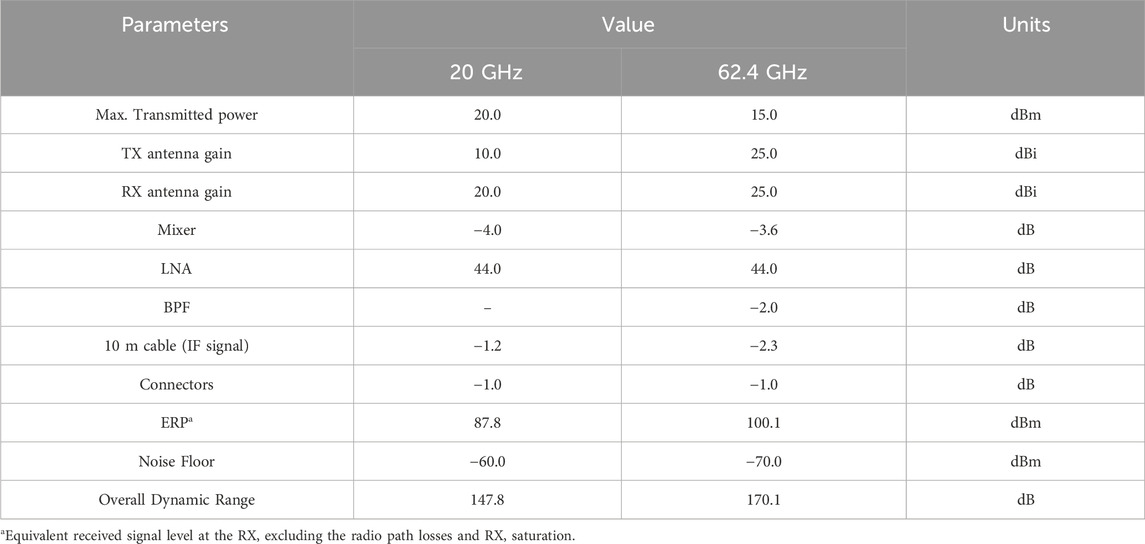
Table 1. Measurement systems’ Link budget.

4 Extension of the 3D ray-tracing based model to doubly-selective vegetated scenarios

In this section, the 3D ray-tracing based model for propagation through vegetation, presented in Leonor et al. (2019), is extended to include the time-varying received signal level, caused by the swaying motion of the tree branches, twigs and leafs. The development of this model extension was based on dynamic re-radiation measurements conducted in a controlled environment, inside an anechoic chamber, which included artificially generated wind from various directions and speeds, at 20 and 62.4 GHz signal frequencies.

A primary model validation is also presented in this section, including the comparison between both measured and simulated time-series of the received signal level, and the comparison of its respective first and secondary order statistics, namely, the cumulative distribution function (CDF), the probability density function (PDF), the average fade duration (AFD), the level crossing rate (LCR) and the autocorrelation function (ACF) received data samples obtained at the various conditions under consideration.

4.1 Methodology and measurement geometry

Measurements intending to record the time-varying re-radiation pattern of a single trees, were conducted inside an anechoic chamber, at 20 and 62.4 GHz. A TX was placed at a distance of 1.70 m from the centre of the tree under measurement (TUM), which is sufficient to ensure plane wave illumination, and the RX was made to rotate around the tree, from $\varphi =-120°$ to $120°$ with $2°$ steps. In each RX step, the received signal level was recorded for a period of one second, at a sampling rate of 10 kHz. Artificial wind was generated from various directions: A to F, as depicted in Figure 5, with different wind speeds: stationary (0 m/s), low (1.9 m/s) and high (4.7 m/s). Figure 6A) depicts the tree used during these experiments, where it’s observable its high leaf density, while Figure 6B) illustrates the measurement scenario from the RX side with visible setups of wind fan at wind positions defined as A and B. Finally, this procedure was repeated for both 20 and 62.4 GHz signal frequencies.

Figure 5

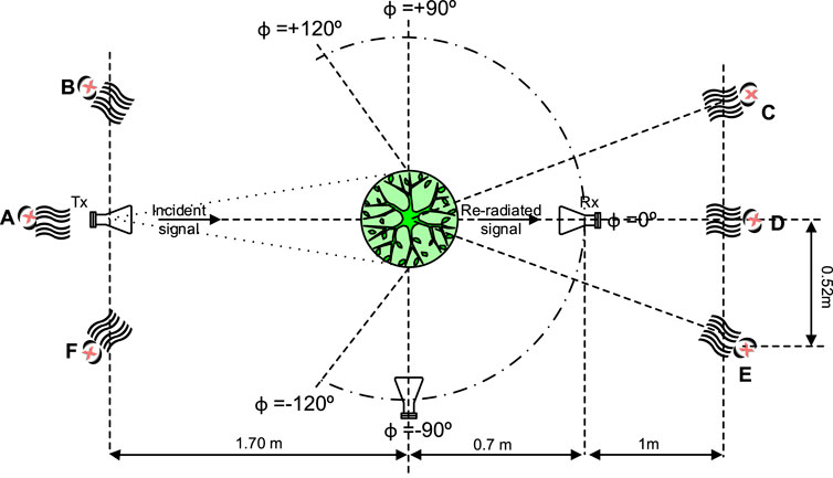
Figure 5. Measurement geometry.

Figure 6

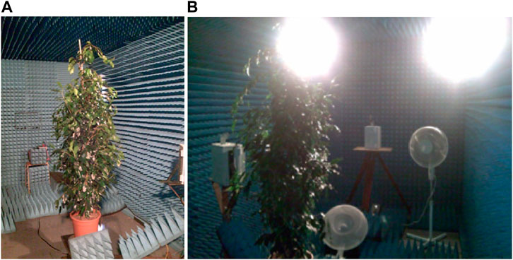
Figure 6. Picture of the measurement scenario: (A) Ficus tree inside the anechoic chamber; and (B) Tree measurement depicted from the receiver side with visible setups of wind fan at wind positions defined as A and B.

Considering the six wind directions (A to F), the three wind speeds (static, low and high), the angular range of the RX rotation (i.e., $-120°$:$2°$:$120°$) and the two signal frequencies, the overall number of time-series extracted using the measurement geometry depicted in Figure 5 is 4,356. These measurements allow the characterisation and modelling of the temporal variations of the received signals due to different wind incidence directions, speeds and bi-static scattering angles.

4.2 Measurement results and statistical analysis

An in-depth statistical analysis on the dynamic measurement results has been conducted. This analysis included the evaluation of the mean and standard deviation (STD) values of the 4,356 different time-series. The normalised mean signal level, with respect to the free space, obtained for wind incidences A and C at 20 GHz are depicted in Figure 7A) and b), respectively, while the same data obtained at 62.4 GHz is depicted in Figure 7C) and d). Figure 8 displays the STD values for same measurement scenarios. As may be observed, there is no evident influence of wind speed on the recorded STD values. Notwithstanding, given the relatively reduced size of the vegetation volume, and the low wind speeds artificially induced inside the anechoic chamber (less that 5 m/s), the obtained STD values are in line with the current International Telecommunication Union - Radiocommunication Sector (ITU-R) recommendation (Assembly, 2013), where STD variations of less than 1 dB were found for wind speeds of 5 m/s.

Figure 7

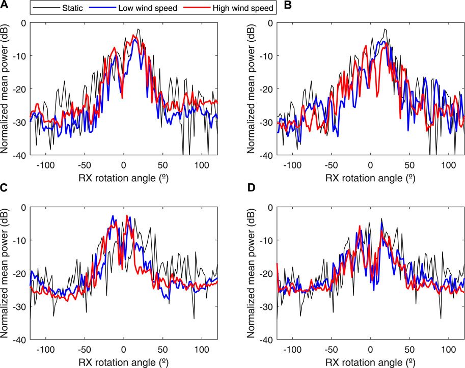
Figure 7. Normalised mean signal level for wind incidences: (A) A at 20 GHz; (B) C at 20 GHz; (C) A at 62.4 GHz; and (D) C at 62.4 GHz.

Figure 8

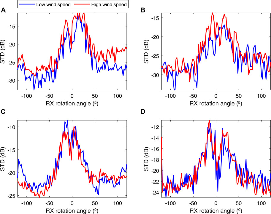
Figure 8. Standard deviation of the signal level for wind incidences: (A) A at 20 GHz; (B) C at 20 GHz; (C) A at 62.4 GHz; and (D) C at 62.4 GHz.

Based on the tree re-radiation pattern and the bi-static scattering angle, three propagation regions can be defined as the RX moves around the vegetation volume in the azimuthal plane. These are (Caldeirinha, 2001): forward scattering $(-30°\le \varphi \le 30°)$, transition ($-45°\le \varphi <-30°$ and $30°<\varphi \le 45$) and side scattering regions ($-120°\le \varphi <-45°$ and $45°<\varphi \le 120°$). These three regions will be further discussed in the characterisation and modelling of the radio channel.

4.3 Propagation model input parameter analysis

Given the availability of the time-series obtained at both RX positions required to apply empirical models (4) and (5), i.e., $\varphi =0°$ and $\varphi =90°$, the first attempt to extend the point scatterer formulation to include wind induced dynamics, was based on the approach adopted in Morgadinho et al. (2012), which relies on time-varying input propagation parameters. Hence, the empirical models (4) and (5) were used to characterise the time-variability of the required input parameters, that is, these empirical models were applied to all the 10 k samples recorded at each step of the dynamic re-radiation measurement, for all the scenarios taken into consideration (Leonor, 2018).

This method was able to provide remarkably accurate representation of the measured signal variability in the forward scattering direction. However, the time-varying $\beta$ parameter proved to be inefficient to characterise the signal variations observed in the side scattering region, i.e., $\varphi =90°$, since it underestimates the measured signal variability. Hence, the $\alpha$ parameter influence on the point scatterers’ re-radiation function, was further investigated.

This analysis consisted of analysing the influence of the $\alpha$ parameter on the front-to-side signal discrimination $(G_{FS})$ of the phase function model. The result of this analysis is depicted in Figure 9, where the $G_{FS}$ values were normalised with respect to the value obtained using $\alpha =0.5$, which is used in the original version of the point scatterer formulation model. As one may observe in Figure 9, the influence of the $\alpha$ parameter on the normalised $G_{FS}$ is relatively constant, regardless of the value used for the $\beta$ parameter. Hence, it is possible to find which $\alpha$ value should be used for a given $G_{FS}$ variation using

${\alpha }_{\mathit{emp}}=0.5+\frac{{\tan }^{-1}\left(\frac{G_{FS}-G_{F{S}_{\mathit{static}}}}{\pi }\right)}{\pi }(6)$

where $G_{F{S}_{\mathit{static}}}$ is the value found for the static wind conditions and the $G_{FS}$ is the recorded time-varying parameter, both expressed in dB. The optimum value of $\alpha$ found on this parametric study as function of the $G_{FS}$ and the empirical model for the $\alpha$ parameter (6) are depicted in Figure 9.

Figure 9

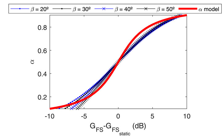
Figure 9. Analysis on the $\alpha$ values to describe the $G_{FS}$ variation.

Using the dynamic measurement data $G_{FS}$ and $I_L$ to extract the time-variant $\alpha$, $\beta$ and $k$ parameters, from Equations 4–6, respectively, the ray-tracing based simulation platform was used to predict the dynamic re-radiation pattern for all the wind incidences, i.e., A to F, for the two wind speed and at both signal frequencies, i.e. 20 and 62.4 GHz.

The results obtained for the normalised power level (NPL) in the forward scattering region for a wind incidence from: a) B with low speed and b) F with high speed at 20 GHz; and c) C with low speed and d) E with high speed at 62.4 GHz, are depicted in Figure 10. As referred previously, the results obtained in the forward scattering direction yielded to a very faithful representation of the measured time-series, since $k$, the most important parameter in this region, is extracted directly from the measured tree insertion loss. Notwithstanding, this analysis proved that the accuracy of the proposed model was not compromised by the introduction of the time-varying $\alpha$.

Figure 10

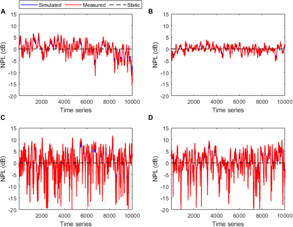
Figure 10. Time series obtained in the forward scattering direction $({\varphi }_{RX}=0°)$ for a wind incidence from: (A) B with low speed and (B) F with high speed at 20 GHz; and (C) C with low speed and (D) E with high speed at 62.4 GHz.

The results with same wind conditions obtained in the side scattering region are depicted in Figure 11. Despite the fact that the time-series representation provided by the proposed model is not as reliable as that obtained in the forward scattering region, the introduction of the time-varying $\alpha$ parameter had lead to significantly better results in the side scattering region, since both measured and simulated NPL variations are now roughly within similar power level ranges.

Figure 11

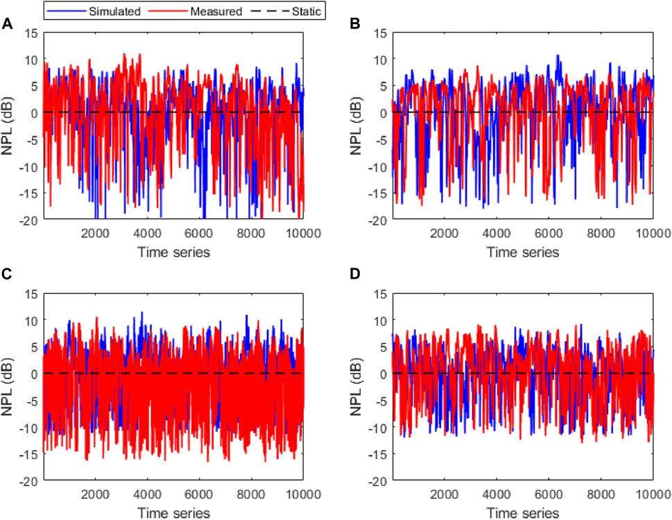
Figure 11. Time series obtained in the side scattering direction $({\varphi }_{RX}=90°)$ for a wind incidence from: (A) B with low speed and (B) F with high speed at 20 GHz; and (C) C with low speed and (D) E with high speed at 62.4 GHz.

The results provided by the proposed dynamic elementary model have been further analysed using first and second order statistics. These include the computation of CDF, PDF, AFD, LCR and ACF of both measured and simulated time-series, for all the scenarios taken into consideration. The results obtained in the forward scattering region $({\varphi }_{RX}=0°)$ with wind incidence from B at low wind speed at 20 GHz, are depicted in Figure 12. As expected after the visual analysis of the time-series depicted in Figure 10, a relatively good agreement between the statistical analysis of both measured and predicted results was achieved, specially in the CDF, LCR and ACF analysis. Similar overall model performance was also achieved in the side scattering region. Results obtained in ${\varphi }_{RX}=90°$ with wind incidence from B with low speed at 62.4 GHz are depicted in Figure 13.

Figure 12

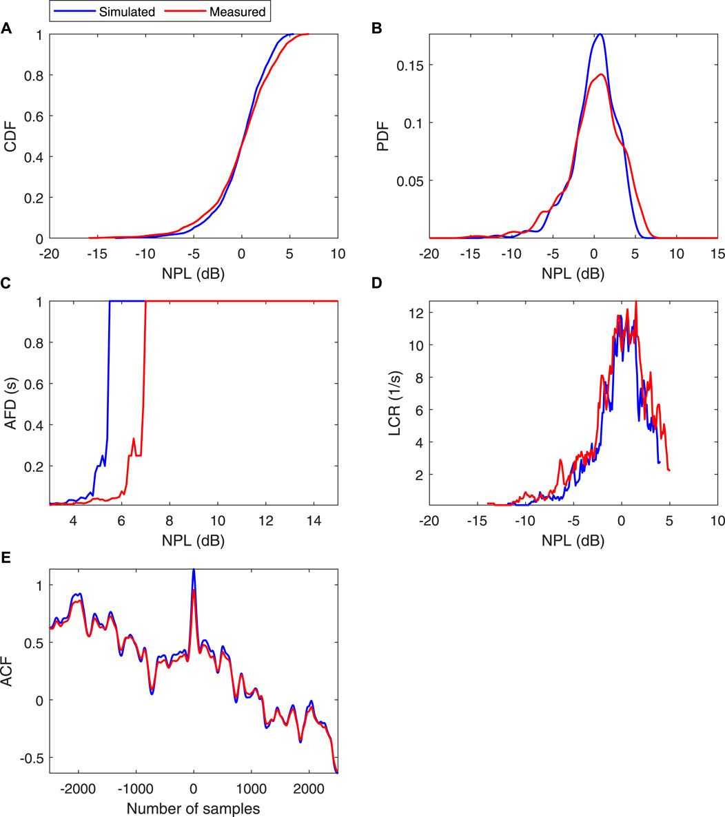
Figure 12. Statistical representation relative to the results obtained in the forward scattering direction $({\varphi }_{RX}=0°)$ with wind incidence from B with low wind speed at 20 GHz: (A) CDF of NPL, (B) PDF of NPL, (C) AFD, (D) LCR and (E) ACF.

Figure 13

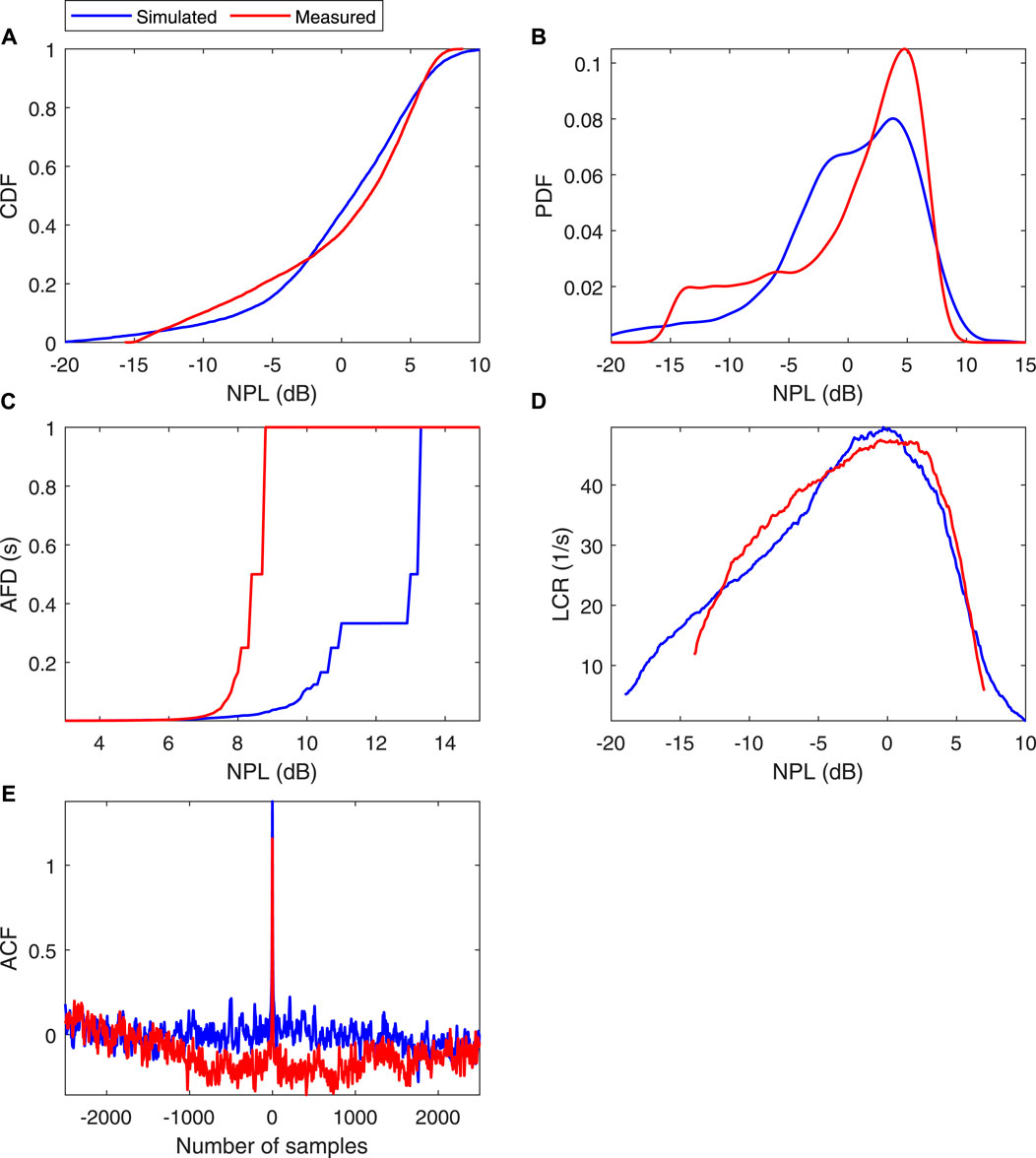
Figure 13. Statistical representation relative to the results obtained in the side scattering direction $({\varphi }_{RX}=90°)$ with wind incidence from B with low wind speed at 62.4 GHz: (A) CDF of NPL, (B) PDF of NPL, (C) AFD, (D) LCR and (E) ACF.

Finally, the Kolmogorov-Smirnov (KS) test was used to assess the degree of similarity between the distribution functions of both measured and simulated time-series of the received signal level. Due to the huge amount of available data, the performance of the proposed model was evaluated in terms of averaged KS test result. Table 2 depicts the averaged KS test results obtained between both measured and simulated time-series. The averaged KS test result was consistently above the 80%, which is a fair good approximation, indicating that the signal level variation caused by the presence of the wind is being properly characterized by the proposed propagation model.

Table 2

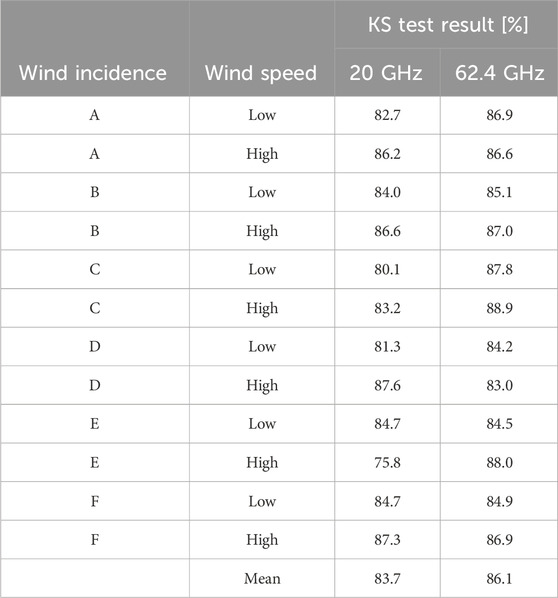
Table 2. Averaged KS test results [%].

4.4 Statistical dynamic model development

Despite the fact that the time-variant input propagation parameters $\alpha$, $\beta$ and $k$, have been proved to be suitable to characterise the signal level variations caused by the wind-induced swaying motion of tree branches and leaves, in both forward and scattering regions, for various wind incidences, two speeds, and two signal frequencies, the model is based on a synchronised input parameter extraction. This means that the time variability of the input propagation parameters must be continuously analysed and extracted so that the signal variations can be properly characterised.

This might cumbersome the model applicability in more complex scenarios, such as tree formations, in which trees present in a formation should primarily be characterised individually, and the extracted input propagation parameters are subsequently used in the ray-tracing algorithm allowing, not only the prediction of the dynamic properties of each individual tree, but also the interactions between different trees present in the simulation channel.

For that purpose, the statistics of the time-variability of the input parameters obtained in the previous section have been further investigated, yielding at the development of a statistical based model, in which the input propagation parameter are defined using random variables with properties of known distributions. This analysis consisted of using the KS test to assess the degree of similarity between the time-varying input parameters with known statistical distributions. With this analysis, it was concluded that the statistical distribution which better characterises the $\alpha$ and $k$ parameters time-variability is the Lognormal distribution, while the Weibull distribution was found to be the most suitable to characterise the $\beta$ parameter variation.

Given the high degree of similarity found between the input parameter variation and these known distributions, the second part of this statistical analysis consisted of finding the specific input values for the these distributions which may generate values for $\alpha$, $\beta$ and $k$ parameters. The Lognormal distribution is defined by the $\mu$ and $\sigma$ parameters, which on a logarithmic scale, are called the location parameter and the scale parameter, respectively, whereas the Weibull distribution uses the scale and shape parameters, $A$ and $B$, respectively. These parameters were then obtained for the specific input propagation parameter datasets and are available in supplementary material of this publication, including the values obtained at 20 and 62.4 GHz, respectively.

The subsequent section will address the performance analysis of this statistical model while characterising the signal level variations found for single and isolated trees under wind influence. To this extent, the input propagation parameters will be defined using the values obtained previously, i.e., acording to Equations 7–9.

$\alpha =\mathbf{L}\left(x,{\mu }_{\alpha },{\sigma }_{\alpha }\right),(7)$

$\beta =\mathbf{W}\left(x,A_{\beta },B_{\beta }\right)\left[°\right](8)$

$k=\mathbf{L}\left(x,{\mu }_k,{\sigma }_k\right)\left[dB/m\right](9)$

where $\mathbf{L}(x,\mu ,\sigma )$ is a random variable with Lognormal distribution with location $\mu$ and scale $\sigma$, and $\mathbf{W}(x,A,B)$ is a random variable with Weibull distribution with scale and shape parameters, $A$ and $B$, respectively.

4.5 Statistical dynamic model validation

The statistical distributions were used to characterise the input propagation parameters time-variability for all the dynamic re-radiation measurement scenarios taken into consideration, that is, wind incidences from A to F, low and high wind speeds, and at 20 and 62.4 GHz signal frequencies. Figure 14 depicts the results obtained at the forward scattering direction for a wind incidence from: a) B with low speed and b) F with high speed, at 20 GHz; and c) C with low speed and d) E with high speed, at 62.4 GHz. Since the model input parameters are now characterised by random variables and hence, they are not extracted directly from the time-varying tree insertion loss, the agreement between both measured and simulated time-series is not as great as that provided by the original dynamic model. This is due to the fast variation nature of a random variable. Similar behaviour was found for the side scattering region results depicted in Figure 15.

Figure 14

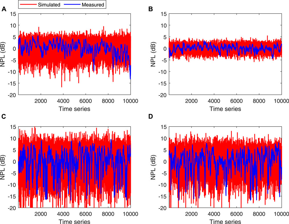
Figure 14. Time series obtained in the forward scattering direction $({\varphi }_{RX}=0°)$ for a wind incidence from: (A) B with low speed and (B) F with high speed at 20 GHz; and (C) C with low speed and (D) E with high speed at 62.4 GHz.

Figure 15

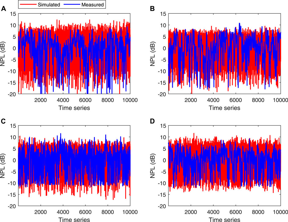
Figure 15. Time series obtained in the forward scattering direction $({\varphi }_{RX}=90°)$ for a wind incidence from: (A) B with low speed and (B) F with high speed at 20 GHz; and (C) C with low speed and (D) E with high speed at 62.4 GHz.

This lack of accuracy on the simulated time-series, specially found in the LCR and ACF analysis, suggests that the input propagation parameters should not be characterised using simple random distribution methods. Nevertheless, despite the overrated signal variation provided by the statistical model, the signal level variations of both measured and simulated time-series are roughly between same level range.

The performance of this statistical based dynamic model have been further analysed, including the evaluation of the first and second order statistics parameters, namely, the CDF, PDF and AFD. LCR and ACF parameters were not included due to the model limitation referred previously. Figure 16 depicts the statistical representation of the results obtained at the forward scattering direction $({\varphi }_{RX}=0°)$ with wind incidence from B with low wind speed at 20 GHz. Disregarding the AFD and LCR, a relatively good agreement between measured and simulated results was achieved for the remaining statistical parameters, specially in the CDFs. This is a remarkable achievement since this statistical model used to characterise the input propagation parameters time variability will enable the application of the dynamic point scatterer formulation to more complex vegetation structures, such as tree formations.

Figure 16

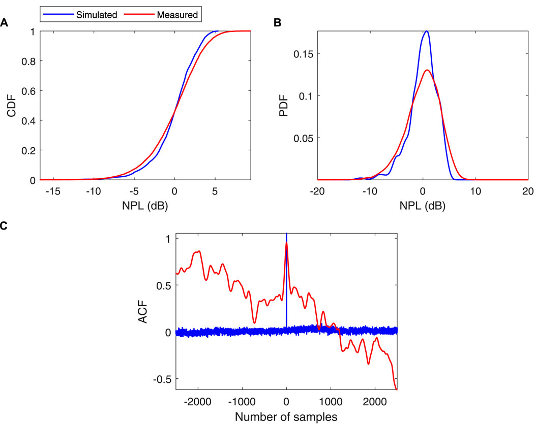
Figure 16. Statistical representation of the results obtained in the forward scattering direction $(\varphi =0°)$ with wind incidence from B with low wind speed at 20 GHz: (A) CDF of NPL, (B) PDF of NPL and (C) ACF.

Similar model performance was found at the side scattering region, in which the simulated signal level is highly affected by the $\alpha$ and $\beta$ time-variability. The statistical representation relative to the results obtained at the side scattering direction with wind incidence from B with low wind speed at 62.4 GHz is depicted in Figure 17. As at the forward scattering direction, the LCR and AFD values found for the side scattering region lack of accuracy due to the fast variation nature of the random variables used to characterise $\alpha$ and $\beta$ parameters. Yet, a relatively good agreement between both measured and simulated CDFs was achieved for this particular scenario.

Figure 17

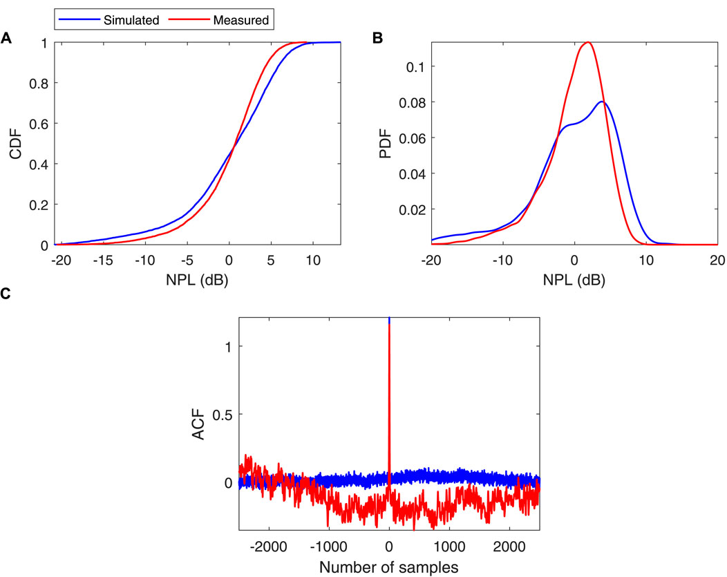
Figure 17. Statistical representation of the results obtained in the side scattering direction $({\varphi }_{RX}=90°)$ with wind incidence from B with low wind speed at 62.4 GHz: (A) CDF of NPL, (B) PDF of NPL and (C) ACF.

For an overview of the overall model performance, the CDF and ACF statistics will be shown in three dimensions accounting for the RX rotation angle, fade or threshold levels and respective statistic magnitude. These will provide an insight view on the overall model performance while predicting the specific time-series with regard to all of the RX rotation angles. Results depicted in Figure 18 concerns to the measured and simulated data obtained with wind incidence from B, with low wind speed, at 20 GHz, whereas the results obtained wind incidence from B, with low wind speed, at 62.4 GHz, are depicted in Figure 19.

Figure 18

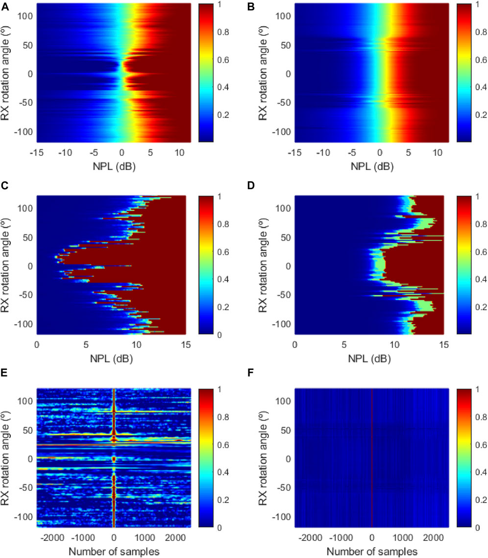
Figure 18. Statistical representation of both measured (left) and simulated (right) of the results obtained with wind incidence from B, low wind speed at 20 GHz. (A) Measured CDF of NPL (B) Simulated CDF of NPL (C) Measured AFD (D) Simulated AFD (E) Measured ACF (F) Simulated ACF.

Figure 19

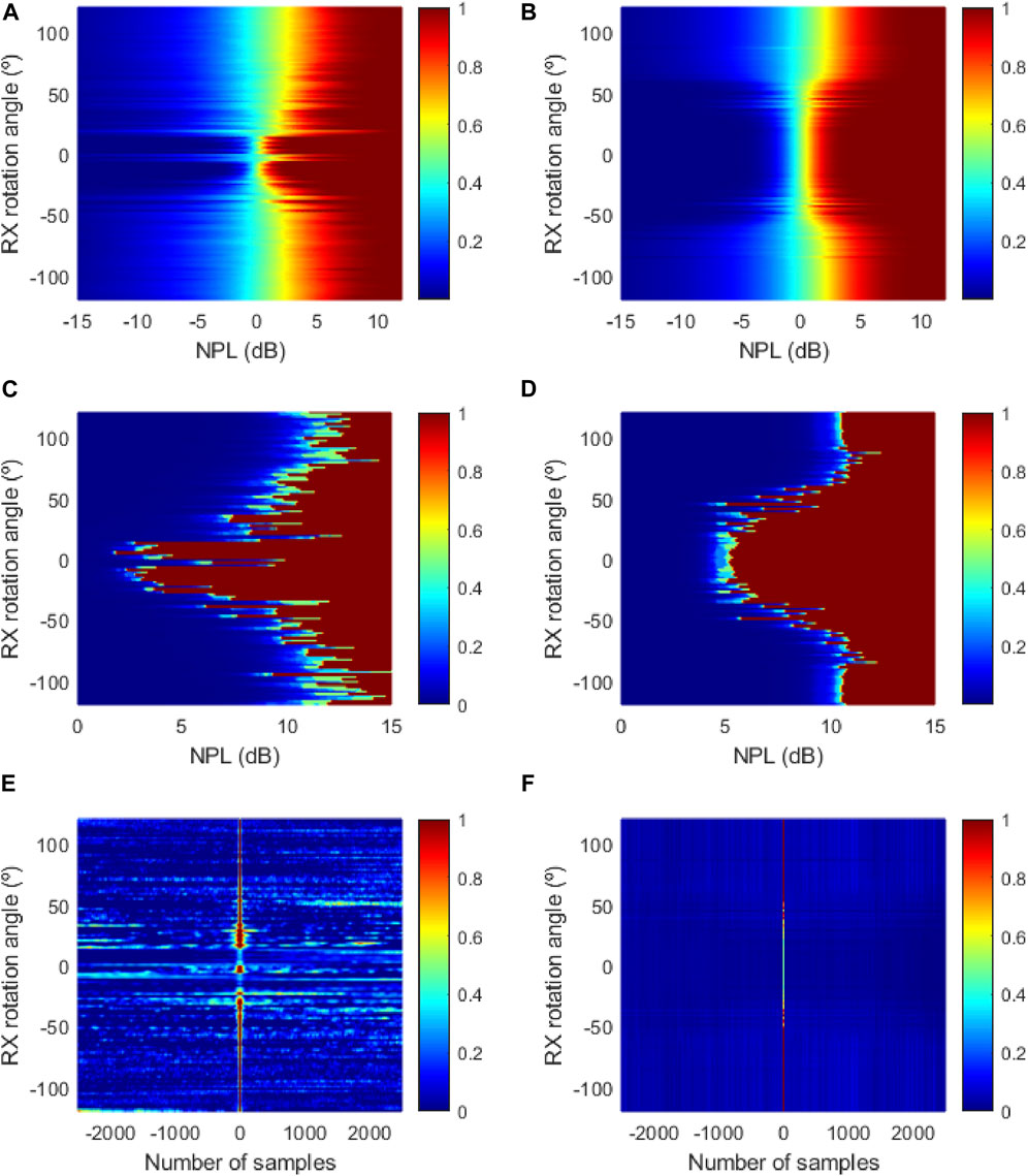
Figure 19. Statistical representation of both measured (left) and simulated (right) of the results obtained with wind incidence from B, low wind speed at 62.4 GHz. (A) Measured CDF of NPL (B) Simulated CDF of NPL (C) Measured AFD (D) Simulated AFD (E) Measured ACF (F) Simulated ACF.

Finally, the simulated time-series were compared against measurement results, using the KS test. Due to the huge amount of available data, the performance of the proposed model was evaluated in terms of averaged KS test result. Table 3 depicts the averaged KS test results obtained between both measured and simulated time-series. The averaged KS test result was consistently above the 80%, which is a fair good approximation.

Table 3

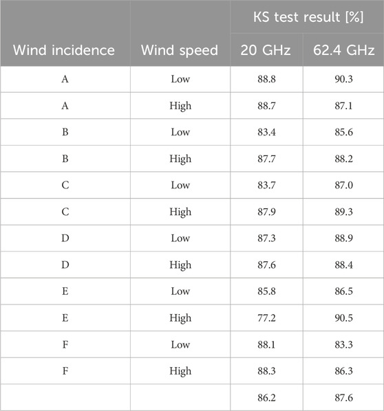
Table 3. Averaged KS test results.

As a final remark to the extension of the point scatterer formulation to include wind-induced dynamics, it is worth to emphasise that the original dynamic model using the input propagation parameters $\alpha$, $\beta$ and $k$, extracted directly and synchronously from dynamic re-radiation measurements, provided a very reliable description and characterisation of the measured time-series. However, its application in tree formation scenarios is inhibited by to the synchronous nature of the input propagation parameters extraction method. On the other hand, the use of known distributions to characterise the time-variability of the input propagation parameters severely decreased the overall model accuracy, particularly in the LCR and AFD analysis. Nevertheless, such method enabled the model application in complex vegetation structures, such as tree formations, in which the distribution parameters, $\sigma$ and $\mu$ for the Lognormal and $A$ and $B$ for the Weibull distributions, may be extracted for a specific tree, and subsequently used to model that tree in a tree formation scenario. Given the these statements, and for the purpose of this research work, the statistical based dynamic model will be assumed to be suitable to characterise the wind induced time-variability of the vegetation environments, and it will be used latter on this document, for the final model validation.

5 Performance analysis in tree formation scenarios under wind influence

This section aims at the validation of the proposed statistical model in more complex scenario, such as tree formation, in which the ray-tracing based simulation platform must, not only to account the time-variability of the received signal level, caused by the swaying motion the branches, twigs and leafs of each tree, but also to account for the signal interaction between different trees and vegetation volumes. To this extend, the proposed statistical model was used to characterise the input propagation parameters $\alpha$, $\beta$ and $k$ of various trees present in a formation, and the directional spectra was simulated for four different RX positions inside the tree structure, for various wind directions and speeds, and at 20 and 62.4 GHz signal frequencies. The performance of the proposed model was subsequently assessed against experimental data obtained in a controlled environment.

5.1 Measurement geometry

Figure 20 depicts the measurement geometry adopted for validation purposes, where the TX was located at 1.4 m from the vegetation structure, composed by 5 Ficus benjamina trees disposed in a $3\times 3$ matrix. At each one of the four RX positions illustrated in Figure 20, the RX was made to rotate around its vertical axis in a $360°$ range, with $2°$ steps. At each step of the RX rotation, the received time-series was recorded over a period of 10 s, with a sampling rate of 1 kHz.

Figure 20

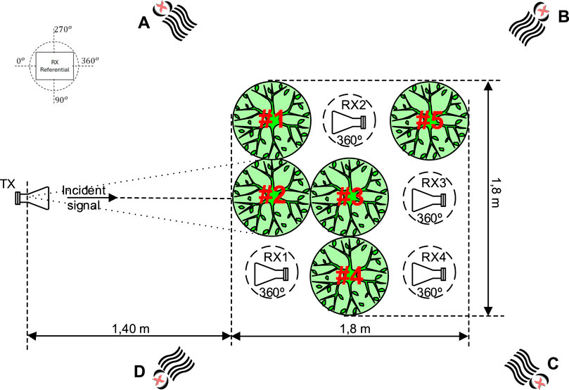
Figure 20. Measurement geometry.

The dynamic directional spectra measurements were conducted in a controlled environment, inside an anechoic chamber, for four different artificially generated wind incidences, A to D, two wind speeds, i.e., low and high, and at 20 and 62.4 GHz signal frequency.

5.2 Simulation geometry

To assess the generic doubly-selective 3D vegetation model based on the point scatterer formulation, a simulation geometry similar to that depicted in Figure 20 was defined. To this extent, the TX was set to a distance of 1.4 m from the first row of trees, represented by the green circles in Figure 21, and four different RX positions were defined according with the measurement geometry. At each one of the RX positions, the $360°$ dynamic directional spectra was simulated using the time-variant input propagation parameters.

Figure 21

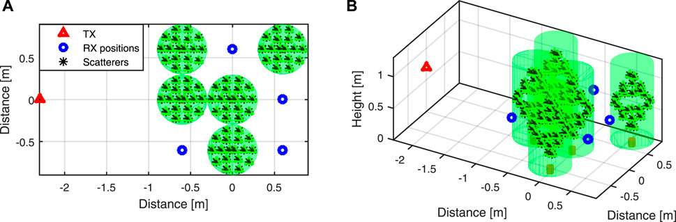
Figure 21. Simulation geometry: (A) top and (B) side views.

The dynamic re-radiation function of each individual tree was not available, therefore the detailed characterisation of the trees present in the simulation channel could not be established. However, all the trees used in the tree formation presented similar characteristics, i.e., height, radius, leaf density, and hence, the statistical parameters obtained for the Tree#1 in Section 4.4 at 20 GHz, were used to model all the trees in the simulation geometry.

5.3 Measurement results and analysis

As referred previously, the statistical based dynamic model overestimates the signal level variation rate, due to the very-fast variation nature of a random variable. Hence, the model performance analysis will be mostly focused in the signal level variation range of both measured and simulated time-series, e.g., CDFs, rather than their variation rate.

Figure 22 depicts both the measured and simulated results obtained at RX position RX1. In this position the RX is in LOS, however, when the RX is pointed to the Tree#2, i.e., ${\varphi }_{RX}=-90°$, the received signal level is more dependent on the wind conditions, since the swaying motion of branches, twigs and leafs, will significantly affect the received signal level. Figure 22 depicts the CDFs of both measured and predicted time-series recorded at RX1 when ${\varphi }_{RX}=-90°$, for the four wind incidences at low speed. From these results, one can conclude that the model accuracy strongly depends on the wind direction, since a poor accuracy was found for wind incidences from B and C, Figure 22B) and c), respectively, a slightly better but still weak agreement between both measured and simulated CDFs, was found for a wind incidence from A, Figure 22A), and a relatively good agreement was found for wind incidence from D, depicted in Figure 22D).

Figure 22

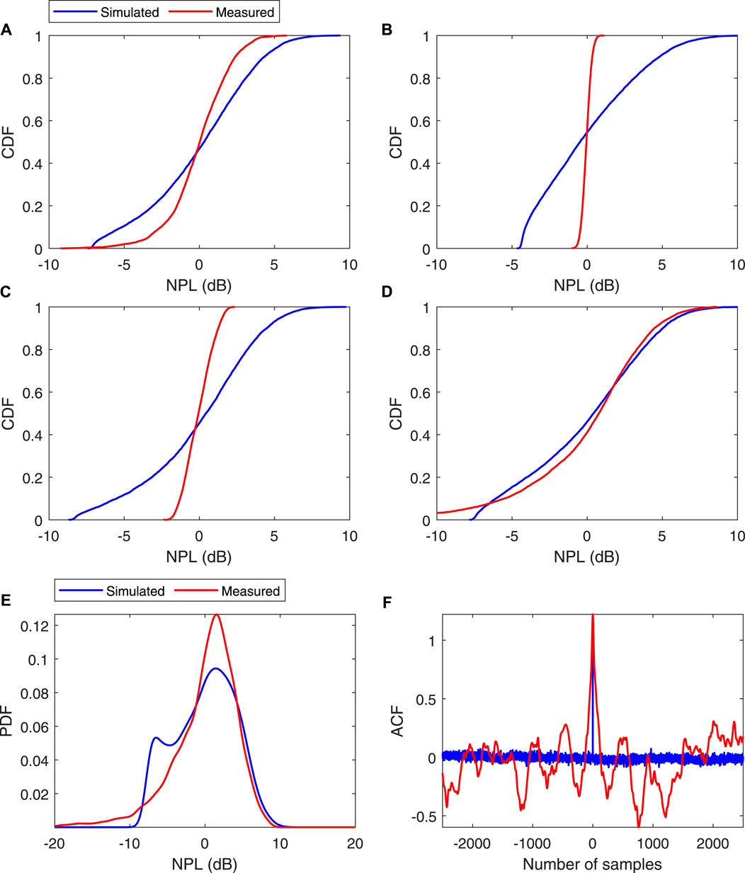
Figure 22. Results obtained for RX position RX1 $({\varphi }_{RX}=-90°)$ at 20 GHz: (A) CDF obtained with low wind speed from A (B) CDF obtained with low wind speed from B (C) CDF obtained with low wind speed from C (D) CDF obtained with low wind speed from D (E) PDF obtained with low wind speed from D, and (F) AFD obtained with low wind speed from D.

This is related with the fact that all the trees in the simulation channel were modelled using time-varying input parameters, i.e., all the trees are assumed to be under wind influence. However, during the wind incidences from B and C, the Tree#2, the one that affects the measurement results the most, is covered by Tree#5 and Tree#4, respectively. Hence, the wind speeds arriving at the Tree#2 are weakened. A similar phenomenon was found for wind incidence from A, in which the wind speed arriving striking the Tree#2 is minimised by the Tree#1. Finally, the wind incidence from D strikes directly on Tree#2, hence, it will cause an enhanced swaying motion the tree branches, twigs and leafs, contributing to an increase of the signal level variation.

A more detailed analysis on the model accuracy while predicting the dynamic effect of the motion of the swaying trees, is depicted in Figure 22E) and f), where the statistical representation of the data recorded in RX position RX1, when pointed at Tree#2, i.e., ${\varphi }_{RX}=-90°$, with wind incidence from D with low speed, is presented, including the PDF and the AFD of both measured and simulated data.

The results obtained at RX2 when pointed directly to the TX, i.e., ${\varphi }_{RX}\approx 20°$, with high wind speeds, are depicted in Figure 23. At this particular position, it was expected that the wind incidence from A would cause a high signal level variation, since both Tree#1 and Tree#2 are swaying. However, the measured signal variations were found in a $\pm$2 dB range. This is related to the fact that the trees used during the measurements, and trees in general, are not homogeneous, and they tend to be sparser near the tree limits. Given the measurement geometry and the RX pointing direction, is most likely that a strong direct component travels between Tree#1 and Tree#2, minimising the wind influence on the received signal level variation. In the proposed propagation model, the tree volume is considered to be homogeneous, and hence the results depicted in Figure 23 do not manifest a great agreement between both measured and simulated data sets.

Figure 23

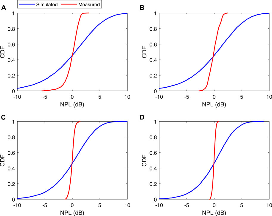
Figure 23. Results obtained for RX position RX2 $({\varphi }_{RX}=20°)$ at 62.4 GHz: (A) CDF obtained with high wind speed from A (B) CDF obtained with high wind speed from B (C) CDF obtained with high wind speed from C (D) CDF obtained with high wind speed from D.

When the RX2 is pointed at Tree#3, i.e., ${\varphi }_{RX}=90°$, and given that all the trees in the simulation channel are assumed to be under wind influence, it is expected that a good agreement between both measured and predicted time-series is achieved for wind incidences from C and D, which strikes directly to that specific tree. A reduced model accuracy is expected for wind incidences from A and B, since the Tree#3 is covered by Tree#1 and Tree#5, respectively. These statements are confirmed by the results depicted in Figure 24, in which the CDF curves obtained for a wind incidence from C, Figure 24C), are almost perfectly matched. Further statistical analysis on the data obtained for RX position RX2, ${\varphi }_{RX}=90°$ with wind incidence from F with high speed is depicted in Figures 24E, F.

Figure 24

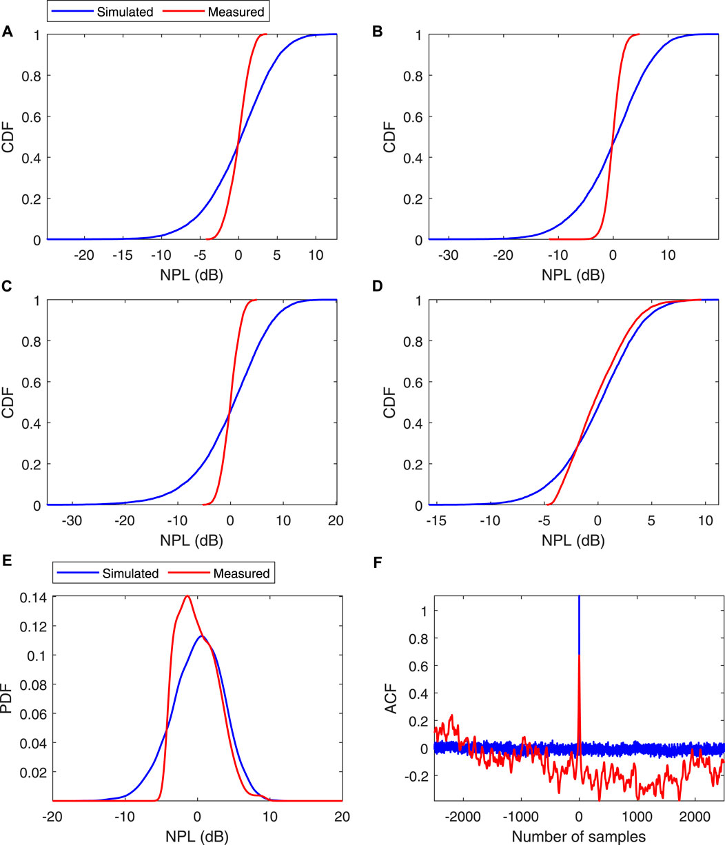
Figure 24. Results obtained for RX position RX2 $({\varphi }_{RX}=90°)$ at 62.4 GHz: (A) CDF obtained with low wind speed from A (B) CDF obtained with low wind speed from B (C) CDF obtained with low wind speed from C (D) CDF obtained with low wind speed from D (E) PDF obtained with high wind speed from F, and (F) AFD obtained with high wind speed from F.

Similar dependence of the overall model accuracy with the wind incidences was found for the remaining RX positions and pointing directions. Results obtained in RX position RX4 pointed at Tree#5, i.e., ${\varphi }_{RX}=-90°$, with high wind speed, are depicted in Figure 25. Given the measurement geometry and the previous results analysis, reliable results are expected for a wind incidence from B, which is consistent with the data provided in Figure 25B). The detailed statistical analysis obtained for this particular measurement scenario is depicted in Figures 25E, F.

Figure 25

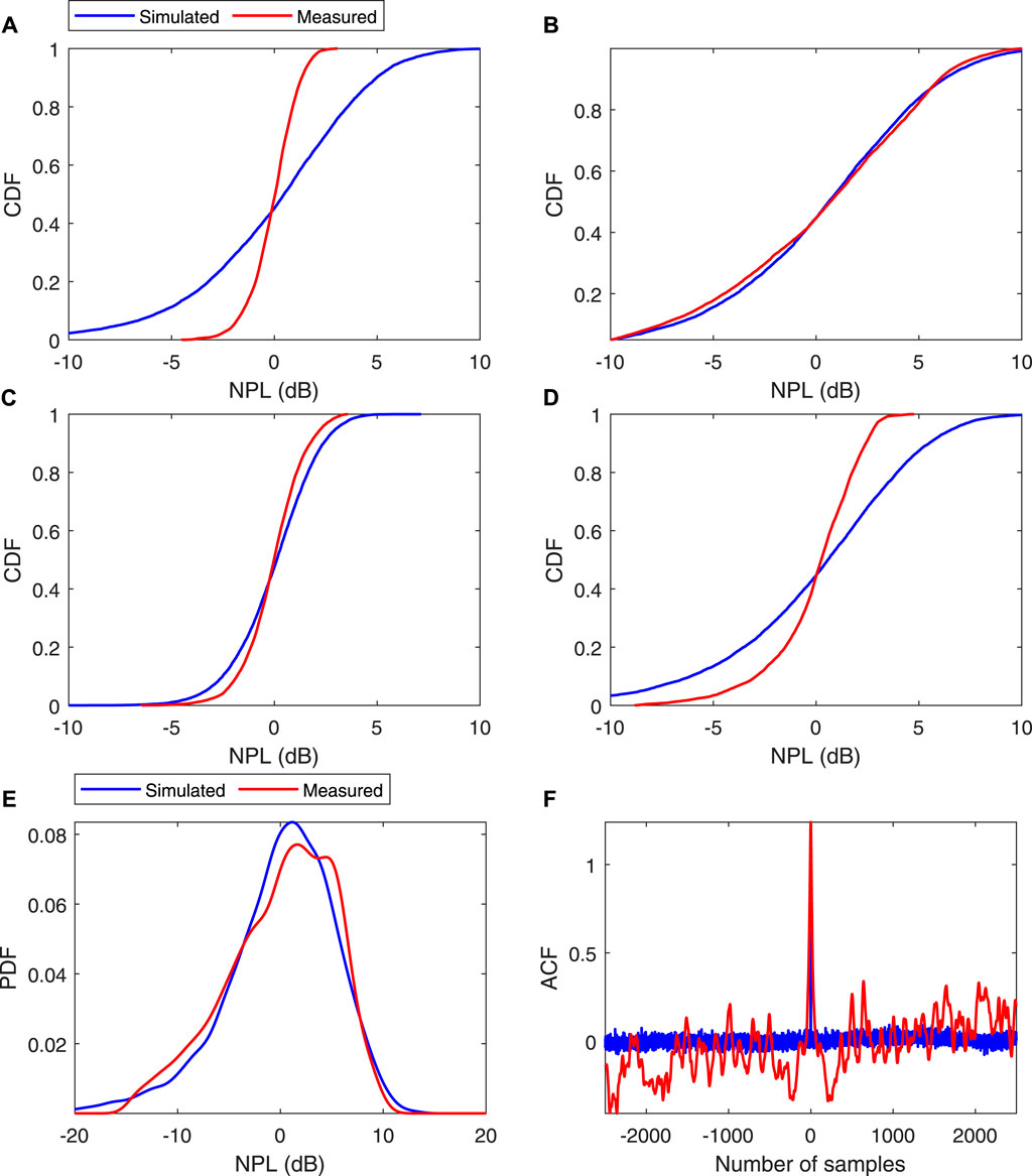
Figure 25. Results obtained for RX position RX4 $({\varphi }_{RX}=-90°)$ at 20 GHz: (A) CDF obtained with high wind speed from A (B) CDF obtained with high wind speed from B (C) CDF obtained with high wind speed from C (D) CDF obtained with high wind speed from D (E) PDF obtained with high wind speed from B, and (F) AFD obtained with high wind speed from B.

6 Conclusion

In this paper, a 3D ray-tracing based doubly-selective model for propagation in vegetation, which accounts for the time-varying effects caused by the wind induced channel dynamics, is proposed. This dynamic model, at the outset, consisted of extracting the empirical input propagation parameters directly and synchronously from measured time-series of the dynamic re-radiation measurements, and yielded to a very reliable description of the signal level variations. However, its application in tree formation scenarios is limited due to the synchronous nature of the input propagation parameters extraction method, since the time instant that the input parameters are extracted, is different than that when the measurements in a tree formation scenario are conducted. Hence, this dynamic model was adapted to be based on the statistics of the signal level variation, in which the time-variability of the input propagation parameters was characterised using known statistical distributions, such as Lognormal and Weibull. Given the very-fast variation nature of a random variable, this second approach provided an accuracy reduction on the estimation of the signal time-series, particularly on the LCR and AFD analysis. However, such method enabled the model application in complex vegetation structures, such as tree formations, in which the distribution parameters, $\sigma$ and $\mu$ for the Lognormal and $A$ and $B$ for the Weibull distributions, may be extracted for a specific tree, and subsequently used to model that tree in a formation scenario. Given this achievement, and the relatively good performance provided by this statistical model, this modelling approach was considered to be suitable to characterise the wind induced effects on vegetated environments, and it was integrated on the doubly-selective vegetation model.

The performance of the doubly-selective vegetation model while predicting the received signal level fluctuations, caused by the wind-induced swaying motion of the tree branches and leaves, in a tree formation scenario, was subsequently assessed against dynamic directional spectra measurements conducted in a controlled environment, inside an anechoic chamber. These measurements were performed at 20 and 62.4 GHz for four RX positions, four different artificially generated wind incidences and two wind speeds, i.e., low and high. The dynamic propagation model proved to be suitable to characterise the time-varying directional spectra providing a good representation of the measured time-series and its first and second order statistics.

The dynamic model developed to account for the wind induced channel time-variability, lacks of accuracy as far as the LCR and AFD analysis are concerned, due to the very-fast variation nature of the random variables used to characterise the time-varying input propagation parameters. Additionally, and as has been proven in Section 4, in tree formation scenarios, the wind will not affect all the trees equally. Thus, to effectively characterise the wind induced time-varying effect in such complex vegetation structures, wind propagation models and its effect on the variability of the input propagation parameters, should also be taken into account.

Data availability statement

The raw data supporting the conclusions of this article will be made available by the authors, without undue reservation.

Author contributions

NL: Writing–original draft, Writing–review and editing. TF: Writing–review and editing. MS: Writing–review and editing. RC: Writing–review and editing.

Funding

The author(s) declare that financial support was received for the research, authorship, and/or publication of this article. This work is part of the project UID/EEA/50008/2023, funded by the Portuguese Foundation for Science and Technology (FCT).

Conflict of interest

The authors declare that the research was conducted in the absence of any commercial or financial relationships that could be construed as a potential conflict of interest.

The author(s) declared that they were an editorial board member of Frontiers, at the time of submission. This had no impact on the peer review process and the final decision.

Publisher’s note

All claims expressed in this article are solely those of the authors and do not necessarily represent those of their affiliated organizations, or those of the publisher, the editors and the reviewers. Any product that may be evaluated in this article, or claim that may be made by its manufacturer, is not guaranteed or endorsed by the publisher.

Supplementary material

The Supplementary Material for this article can be found online at: https://www.frontiersin.org/articles/10.3389/fanpr.2025.1417976/full#supplementary-material

References

Assembly (2013). Radiocommunication. Recommendation itu-r p. 833-8, attenuation in vegetation. ITU-R.

Google Scholar

Caldeirinha, R. (2001). “Radio Charaterisation of single trees at micro- and millimetre wave frequencies,”. Ph.D. thesis (UK: University of Glamorgan).

Google Scholar

Caldeirinha, R., Fernandes, T., Leonor, N., and Ferreira, D. (2010). “Extension of the dret model to include scattering from tree trunks in microcell urban mobile scenarios,” in Proc. IEEE vehicular Technology conference (VTC-Spring) (Taipei, Taiwan).

Google Scholar

International Radio Consultative Committee (1986). Influences of terrain irregularities and vegetation on tropospheric propagation. Reports and recommendations of the CCIR, 236–6.

Google Scholar

Chee, K., Torrico, S., and Kurner, T. (2013). Radiowave propagation prediction in vegetated residential environments. IEEE Trans. Veh. Technol. 62, 486–499. doi:10.1109/tvt.2012.2226764

CrossRef Full Text | Google Scholar

COST235 (1995). Radio propagation effects on next-generation fixed-service terrestrial Telecommunications systems. Luxembourg: Final Report.

Google Scholar

Didascalou, D., Younis, M., and Wiesbeck, W. (2000). Millimeter-wave scattering and penetration in isolated vegetation structures. IEEE Trans. Geoscience Remote Sens. 38, 2106–2113. doi:10.1109/36.868869

CrossRef Full Text | Google Scholar

Fernandes, T. (2007). “A discrete RET model for micro- and millimetre wave propagation through vegetation,”. Ph.D. thesis (U.K: University of Glamorgan).

Google Scholar

Fernandes, T., Caldeirinha, R., Al-Nuaimi, M., and Richter, J. (2005). A discrete ret model for millimeter-wave propagation in isolated tree formations. IEICE Trans. Commun. E88-B, 2411–2418. doi:10.1093/ietcom/e88-b.6.2411

CrossRef Full Text | Google Scholar

Johnson, R., and Schwering, F. (1985). A transport theory of millimeter wave propagation in woods and forest. Technical Report CECOM-TR-85-1.

Google Scholar

Leonor, N. (2018). “A generic doubly-selective 3D vegetation model using point scatterers,”. Ph.D. thesis (Spain: Univ. of Vigo).

Google Scholar

Leonor, N., Caldeirinha, R., Fernandes, T., Ferreira, D., and Sánchez, M. (2014). A 2d ray-tracing based model for micro- and millimeter-wave propagation through vegetation. IEEE Trans. Antennas Propag. 62, 6443–6453. doi:10.1109/tap.2014.2362124

CrossRef Full Text | Google Scholar

Leonor, N., Caldeirinha, R., Sanchez, M., and Fernandes, T. (2017). A two-dimensional ray-tracing-based model for propagation through vegetation: a practical assessment using ornamental plants at 60 GHz. [Wireless corner]. IEEE Antennas Propag. Mag. 59, 145–150. doi:10.1109/map.2016.2629839

CrossRef Full Text | Google Scholar

Leonor, N., Fernandes, T., Garcia Sanchez, M., and Caldeirinha, R. F. S. (2019). A 3d model for millimeter-wave propagation through vegetation media using ray-tracing. IEEE Trans. Antennas Propag. 67, 4313–4318. doi:10.1109/tap.2019.2905957

CrossRef Full Text | Google Scholar

Leonor, N., Sanchez, M., Fernandes, T., and Caldeirinha, R. F. S. (2018). A 2d ray-tracing based model for wave propagation through forests at micro and millimeter wave frequencies. IEEE Access 6, 32097–32108. doi:10.1109/access.2018.2836223

CrossRef Full Text | Google Scholar

Meng, Y., Lee, Y., and Ng, B. (2009). Empirical near ground path loss modeling in a forest at vhf and uhf bands. IEEE Trans. Antennas Propag. 57, 1461–1468. doi:10.1109/tap.2009.2016703

CrossRef Full Text | Google Scholar

Morgadinho, S., Caldeirinha, R., Al-Nuaimi, M., Cuinas, I., Sanchez, M. G., Fernandes, T. R., et al. (2012). Time-variant radio channel characterization and modelling of vegetation media at millimeter-wave frequency. IEEE Trans. Antennas Propag. 60, 1557–1568. doi:10.1109/tap.2011.2180301

CrossRef Full Text | Google Scholar

Rogers, N. C., Seville, A., Richter, J., Ndzi, D., Savage, N., Caldeirinha, R. F. S., et al. (2002). A generic model of 1-60 GHz radio propagation through vegetation - final report. UK: QINETIQ/KI/COM/CR020196/1.0.

Google Scholar

Seville, A., and Craig, K. (1995). Semi-empirical model for millimetre-wave vegetationattenuation rates. Electron. Lett. 31, 1507–1508. doi:10.1049/el:19951000

CrossRef Full Text | Google Scholar

Torrico, S., Bertoni, H., and Lang, R. (1998). Modeling tree effects on path loss in a residential environment. IEEE Trans. Antennas Propag. 46, 872–880. doi:10.1109/8.686776

CrossRef Full Text | Google Scholar

Torrico, S., and Lang, H. (2012). “Wave attenuation prediction through a volume of random located lossy-dielectric branches – 3-d vector transport theory,” in 6th European conference on antennas and propagation (EUCAP) (prague), 3342–3345.

Google Scholar

Ulaby, F., Haddock, T., and Kuga, Y. (1990). Measurement and modeling of millimeter wave scattering from tree foliage. Radio Sci. 25, 193–203. doi:10.1029/rs025i003p00193

CrossRef Full Text | Google Scholar

Wang, F. (2006). “Physics-based modeling of wave Propagation for terrestrial and space communications,”. Ph.D. thesis (USA: University of Michigan).

Google Scholar

Wang, F., and Sarabandi, K. (2005). An enhanced millimeter-wave foliage propagation model. IEEE Trans. Antennas Propag. 53, 2138–2145. doi:10.1109/tap.2005.850704

CrossRef Full Text | Google Scholar

Wang, F., and Sarabandi, K. (2007). A physics-based statistical model for wave propagation through foliage. IEEE Trans. Antennas Propag. 55, 958–968. doi:10.1109/tap.2007.891841

CrossRef Full Text | Google Scholar

Weissberger, M. (1982). An initial critical summary of models for predicting the attenuation of radio waves by trees. Technical Report ESD-TR-81-101 Department of Defense.

Google Scholar