Machine learning algorithms for the prediction of EUROP classification grade and carcass weight, using 3-dimensional measurements of beef carcasses

Introduction: Mechanical grading can be used to objectively classify beef carcasses. Despite its many benefits, it is scarcely used within the beef industry, often due to infrastructure and equipment costs. As technology progresses, systems become more physically compact, and data storage and processing methods are becoming more advanced. Purpose-built imaging systems can calculate 3-dimensional measurements of beef carcasses, which can be used for objective grading.

Methods: This study explored the use of machine learning techniques (random forests and artificial neural networks) and their ability to predict carcass conformation class, fat class and cold carcass weight, using both 3-dimensional measurements (widths, lengths, and volumes) of beef carcasses, extracted using imaging technology, and fixed effects (kill date, breed type and sex). Cold carcass weight was also included as a fixed effect for prediction of conformation and fat classes.

Results: Including the dimensional measurements improved prediction accuracies across traits and techniques compared to that of results from models built excluding the 3D measurements. Model validation of random forests resulted in moderate-high accuracies for cold carcass weight (R2 = 0.72), conformation class (71% correctly classified), and fat class (55% correctly classified). Similar accuracies were seen for the validation of the artificial neural networks, which resulted in high accuracies for cold carcass weight (R2 = 0.68) and conformation class (71%), and moderate for fat class (57%).

Discussion: This study demonstrates the potential for 3D imaging technology requiring limited infrastructure, along with machine learning techniques, to predict key carcass traits in the beef industry.

Introduction

Within the livestock industry, new automated practices can be implemented at different stages of the supply chain from farm to fork, with various technologies being available to improve efficiency post-slaughter, for example during carcass processing. This includes the automation of carcass grading, which has the potential to improve profitability while reducing emissions, both on-farm and in the abattoir.

Currently in the UK, carcasses are graded using the EUROP carcass classification grid, where the conformation (shape) and fat coverage of a carcass are assessed (Strydom, 2022). Conformation classes range from E to P, with E representing carcasses of excellent shape and P carcasses of poor shape, and fat classes range from 1–5, with one being low, and five being excessive levels. Each class has the potential to be subdivided into one of three subclasses (plus, equal or minus), allowing for one of 15 potential conformation and fat classes to be assigned (15-point scale). The two classes are combined to give an overall grade, and this determines the price paid to the producer in pence per kilogram (UK GBP) of the carcass. With mechanical grading, the 15-point scale is used, allowing for one of 225 potential grades to be awarded to the overall carcass (AHDB, 2024). However, many abattoirs rely on manual (visual) grading when classifying carcasses, and with this method, different countries across Europe implement different combinations of the subclasses. For example, in the UK, plus and minus subclasses are only used for conformation classes U, O, and P and fat classes 4 and 5, and only equal subclasses are used for conformation classes E and R and fat classes 1, 2 and 3 (traditional grid). Regardless of the grid used, cattle of grades that represent the market specifications more closely result in higher prices, while lower prices result from cattle of poor conformation or high fat classes, with the latter often associated with over-finished animals. Therefore, ensuring cattle are sent to slaughter at the optimum grade has the potential to reduce emissions resulting from over-finished animals (i.e., emissions from excess inputs and excess enteric methane production) and improve profitability due to the premium prices being met.

It has been recognized, however, that the subjective nature of visual grading can lead to a lack of trust in the classification system (Allen and Finnerty, 2000). This is due to the fact that the grades awarded may be influenced by many factors, such as the classifier and their experience (Wnęk et al., 2017), the time of day, or prior carcasses. This may reduce the financial incentive for producers to finish their cattle at the optimum slaughter date, and therefore objective techniques must be adopted. Despite this, they are not widely utilized in the UK, which may be due to only one system (VBS2000, e + v technology, Oranienburg, Germany) being approved for commercial use under government guidance. This system is integrated into the slaughter line, and images are captured of the carcass side, which has raster stripes projected onto it, indicating the contour of the carcass for the shape (conformation) to be assessed. The quantity of red and white flesh is compared for the estimation of fat class. To ensure this process works effectively, the system requires 9.2m of floor space to cater for the associated infrastructure (Craigie et al., 2012). It may not always be favorable for abattoirs to sacrifice this space for the technology, particularly when the costs associated with purchasing and installing the equipment are factored in. Therefore, visual grading is still favored in many abattoirs and the final grades, and therefore prices paid to farmers, are decided subjectively.

In order to encourage the adoption of mechanical grading systems, technology requiring limited infrastructure, resulting in lower costs, must be made available. Although large amounts of infrastructure were previously needed for technologies to extract the necessary information of the carcass for objective grading (e.g., 3D information), advancements have not only made more complex technology more affordable, but also more compact. Therefore, 3D information can be extracted from small, purpose-built systems requiring limited infrastructure, reducing the cost and space required. This is the case with time-of-flight cameras, which can produce point cloud images, allowing for 3D information to be generated using the camera alone (Hansard et al., 2013). Along with new technology, novel approaches for analyzing data are also available, such as machine learning. Previously, techniques such as linear regression were used for predictive analytics, however, advancements in technologies have allowed for real-time analysis of big data. Machine learning aims to mimic that of humans in terms of learning from the environment, either for predictions (supervised machine learning techniques) or pattern recognition (unsupervised machine learning) (Liakos et al., 2018), and machine learning has been widely adopted in the agricultural industry in recent years, aiding the monitoring of crop, water, soil, and livestock management (Benos et al., 2021). There are many benefits associated with machine learning compared to that of traditional statistics (e.g. linear regression), with machine learning in particular being helpful for analyzing data where the number of inputs exceed the number of outputs (Bzdok et al., 2018) or where outputs are categorical (Goyache et al., 2001). Despite this, machine learning methods have been noted to be more “sophisticated” than that of linear formulas (Goyache et al., 2001), resulting in what is often referred to as a “black box” approach (Alves et al., 2019). This can lead to a lack of understanding of how the algorithm reaches its final prediction and which features of an observation led to the prediction. This is particularly true with methods such as artificial neural networks where there are input and output layers, with a series of hidden layers between, and thus it has been noted that there is no automatic procedures to estimate suitable artificial neural network architecture (Goyache et al., 2001). Despite these potential negatives, studies have found that various machine learning techniques often outperform linear regression when predicting carcass traits (Alves et al., 2019; Miller et al., 2019; Shahinfar et al., 2019), indicating the potential for their implementation within the grading industry, assuming suitable and practical technology is provided.

The objective of this study was to assess the ability of 3D measurements extracted from images of beef carcasses, combined with machine learning algorithms, to predict key carcass traits. The images were obtained from a time-of-flight camera, which required limited infrastructure. Extracted 3D measurements were included, along with other fixed effects (carcass details), to predict carcass conformation, fat class and cold carcass weight (CCW), using machine learning algorithms. Two supervised machine learning techniques were compared, as well as results from models built using basic fixed effects (kill date, breed type, sex, and CCW for the prediction of conformation and fat class) or a combination of fixed effects and 3D measurements.

Materials and methods

Data were collected from 33,730 beef carcasses at one commercial abattoir in Scotland. Data from a total of 89 different breeds and crosses were recorded, across 106 days between 16th of April 2022 and the 6th of October 2022. On average, data were collected for 318 carcasses per day.

Carcass processing

At the abattoir cattle were stunned by captive bolt and exsanguinated as each carcass was hooked to an automatic track conveyor (kill line). The carcasses were then dressed and eviscerated, following standard abattoir practice, to UK specification (see Meat and Livestock Commercial Services Limited beef authentication manual, www.mlcsl.co.uk, for full description). The carcasses were split down the midline, with each half being individually hooked to the conveyer by the achilleas. The carcasses then moved down the kill line, passing in front of the camera immediately prior to grading, where 7 seconds worth of video was captured per carcass. After image capture the carcasses were manually graded, and any excess flesh and fat was then trimmed before butchery.

3D image capture

A Basler Blaze (Basler Inc., Exton, PA, USA) time-of-flight near infra-red camera (housing size 100mm x 81mm x 64mm) collected the image data of the carcasses. The camera used infrared light beams to generate 3D point cloud images of the external surface of the right-hand side of the carcass. A total of 35 3D image frames were captured for each right-hand side of the carcass (seven seconds worth of video, with five frames captured per second). In addition to the camera, a 1.6m-wide steer bar was positioned behind the carcasses, 2m above the ground. This was the only other required infrastructure and was installed to reduce the risk of the carcasses rotating while images were being captured.

Visual grading

After the carcasses moved on from image capture, they were graded manually for both conformation class and fat class. The grade awarded was assigned from the traditional EUROP classification grid used within the UK, by a trained assessor. While the carcasses were being graded, the hot carcass weight was automatically recorded using a suspension weigh scale installed on the line. Two percent of the hot carcass weight was subtracted to give the value for the CCW.

Image processing and 3D measurement calculation

The 3D point cloud frames were processed by Innovent Technology Ltd., through algorithms developed using Halcon Image Processing Library (MVTech Software GmbH, Munich, Germany). The algorithms generated a single edge contour (outline) of the right-hand side of the carcass and from that a series of 3D measurements were extracted. Although 35 frames were captured per carcass, it was not always possible for every frame to be processed, due to unclear images resulting from noise caused by the carcass swinging horizontally. A total of 713,090 images were processed from 33,730 carcasses and 44 measurements (5 lengths, 18 widths and 21 volumes) were extracted from each frame (Figure 1; Table 1) and used to build the machine learning algorithms.

Figure 1

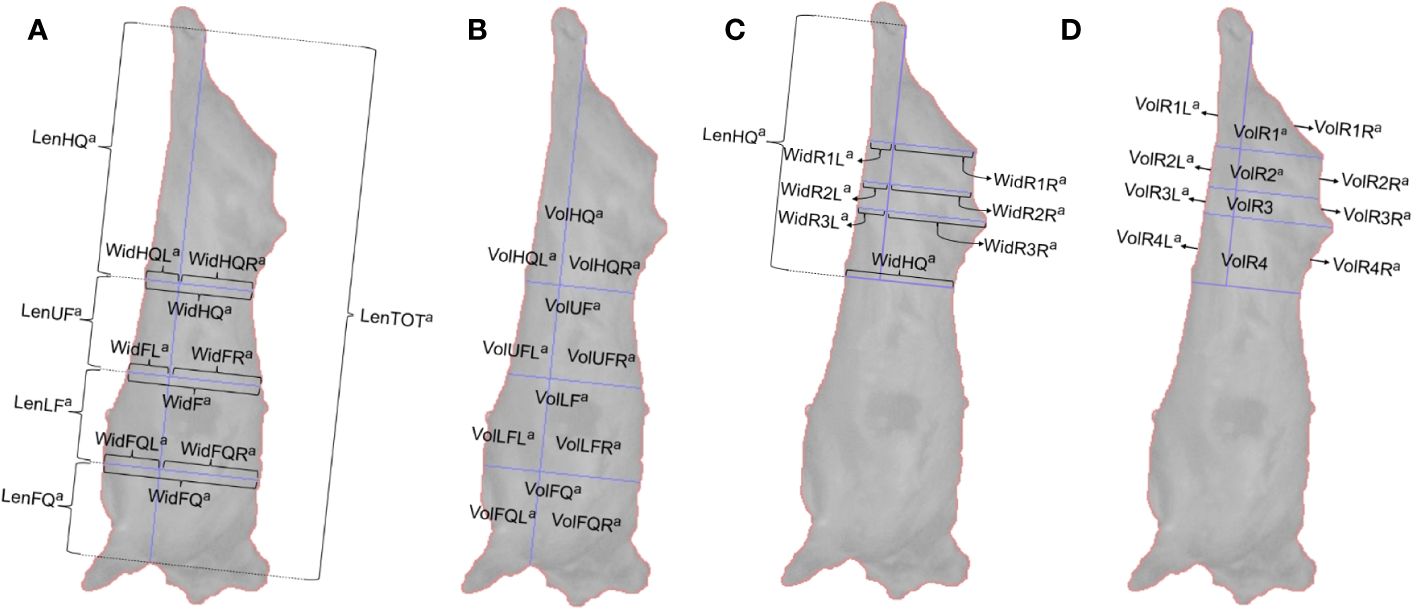
Figure 1 (A) Length and width measurements extracted from images of the carcass, (B) volume measurements extracted from images of the carcass, (C) width measurements of the rump extracted from images of the carcass, (D) volume measurements of the rump extracted from images of the carcass.

Table 1

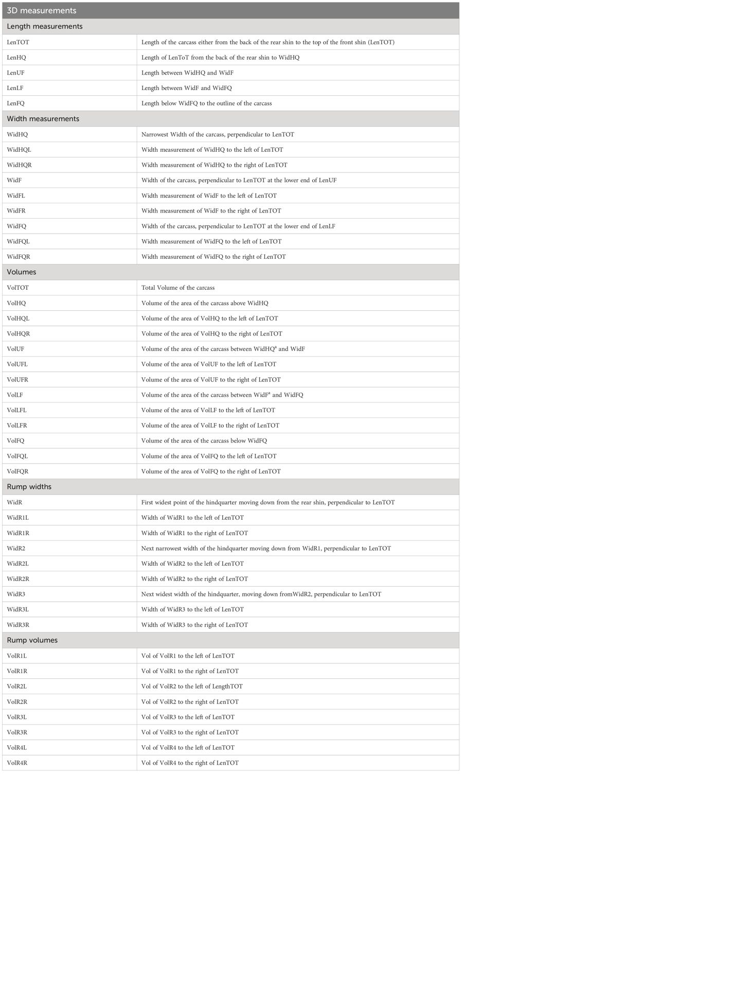
Table 1 Three-dimensional (3D) measurements extracted from the carcass.

The locations on the carcass where the 3D measurements were taken from were selected based upon findings from literature searches (Borggaard et al., 1996; Bozkurt et al., 2008; Rius-Vilarrasa et al., 2009; Emenheiser et al., 2010; De La Iglesia et al., 2020; Stinga et al., 2020). The width and length measurements were extracted from locations that allowed the carcass side to be separated into the hindquarter, flank and forequarter, due to the role these sections play in both butchery and grading. An axis based on anatomical features of the carcass, measuring from the back of the rear shin to the top of the front shin, provided a total length measurement of the carcass and the rest of the 3D measurements were extracted relative to this axis. Widths were measured perpendicular to the axis (Figure 1A), with the width of the hindquarter being identified as the narrowest width of the carcass and two further width measurements were extracted at equal spacing below the narrowest width and the lowest point of the axis. Smaller subsections of each measurement were also recorded, which were identified by points where measurements crossed, for example widths to the left/right-hand side of the total length axis. Volumes were extracted from within the carcass outline (Figure 1B). Smaller individual volumes were extracted, again defined by subsections determined by the lines drawn to measure widths and the axis. An additional series of width measurements (Figure 1C) and volume measurements (Figure 1D) were extracted from the hindquarter of the carcass. These measurements were selected due to the rump region of the carcass appearing susceptible to changes across the classification grades when assessed visually.

Preliminary data inspection and data cleaning

The 3D measurements extracted from the carcass images were imported into RStudio, V4.2.3 (RStudio, Boston, MA, USA). Quality assurance measures put in place by Innovent technology Ltd., identified 407,770 of the 713,090 images as unsuitable for analysis, due to issues such as the carcass side rotating, or members of the abattoir’s workforce being included in the image processing. Along with this, it was observed that the flank tissue on some carcasses was severed during dressing. This resulted in abnormalities in carcass presentation (Figure 2A) compared to that of carcasses that had not been cut (Figure 2B), impacting measurements. For this reason, carcasses that had the flank severed were also removed from further analysis.

Figure 2

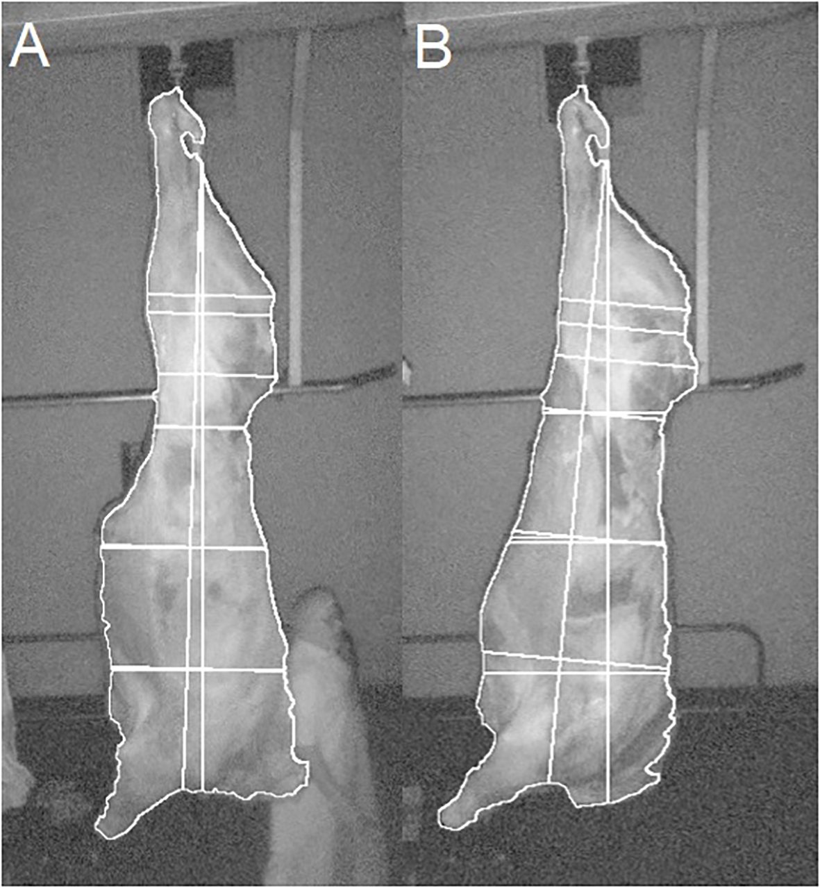
Figure 2 Example images of carcasses and extracted measurements, with (A) flank tissue cut and (B) flank tissue not cut.

Carcass details collected by the abattoir (such as the carcass classification grade, weight, eartag number (UKID), sex and breed) were stored in a SQL server management database (version SQL Server 2014, Microsoft, Washington, USA), and were imported into RStudio to be joined with the measurements of any corresponding carcasses. Only images for steers and heifers were considered for analysis.

The measurements extracted from the remaining 305,320 images for 19,186 carcasses were used to build density plots to test for normal distribution. Any measurement values that were identified as obvious outliers were removed. The mean and standard deviation values were calculated for each measurement using the remaining values. Any values outwith 5 standard deviations above or below the mean of each measurement were also removed, leaving 285,109 images for 17,250 carcasses (Table 2).

Table 2

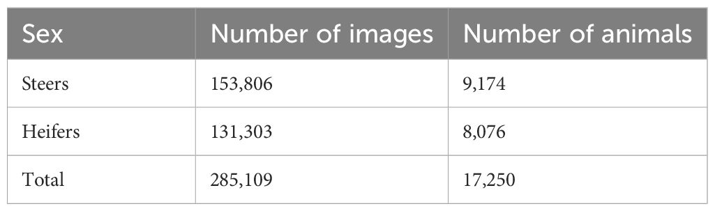
Table 2 Number of datapoints (images) and animals in the final dataset.

The most common manually recorded classification grade in the final dataset was R4L (n=6,104). Few carcasses of the extreme grades (E+, P+, P−, 1, 5L, 5H) were recorded (Table 3). The breed of the carcass, which was recorded as a breed code categorized under the cattle tracing system (British Cattle Movement Service, 2014), was also converted to a simplified breed type category (cattle of either Continental or British descent).

Table 3

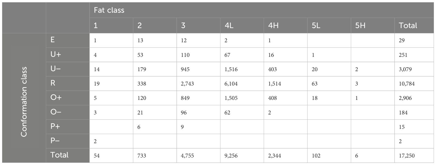
Table 3 Number of each grade awarded for all carcasses in the final dataset.

Data analysis

A minimum of one and up to thirty-five 3D images were captured per carcass, resulting in an average number of 16 useable images per animal. Coefficients of variation (CV) were calculated for each dimensional measurement per carcass to assess variation from measurements extracted across images of each carcass. The majority of carcasses had a low CV for each measurement (average across all images <0.3) between frames and consistent levels of variability were noted across the 3D measurements. For this reason, the values within each 3D measurement were averaged using the arithmetic mean over all suitable images for each carcass, resulting in one row of data per carcass, each containing 3D measurements, conformation class, fat class, cold carcass weight and fixed effects (breed, sex, and kill date) for further analysis. For each of the three carcass traits (carcass conformation, fat class and CCW), separate training and validation datasets were created, containing 70% and 30% of the datapoints respectively. For the prediction of conformation and fat class, as the dependent variables were categorical, the data were split using stratified random sampling, selecting 70% of datapoints from each class, ensuring each class was represented in the training dataset. The CCW was also included as fixed effect for the prediction of conformation and fat class, therefore this variable was included in these datasets. Random sampling was used to split the data for the prediction of CCW as this was continuous. The split of carcasses remained the same for all models per trait. The data were then analyzed using two supervised machine learning methods: Random Forest (RF) and artificial neural network (ANN) models in RStudio, version 2023.03.1 + 446 (R Core Team, 2023).

Random forests

The “train” function from the “caret” package (Kuhn, 2008) was used to build the RF models using the training dataset for each respective carcass trait. For all RF models built, roughly two thirds of the data in the training dataset is automatically sampled randomly with replacement to build numerous trees in the model. These are referred to as bootstrap samples. In some trees an observation may be included in the bootstrap sample more than once, or not at all. The outcomes across all trees are then averaged to give the final result from the RF. The data that were not included in the bootstrap samples are known as the out-of-bag (OOB) sample, and this can be used to estimate the error rate of the model, by calculating the percentage of incorrect predictions (Breiman, 2001). A 10-fold cross validation repeated three times was used to validate each RF model built in the training process and the type of algorithm was set to “Classification” for the prediction of conformation and fat class, or “Regression” for the prediction of CCW. The parameters of the algorithm were the number of trees per RF (ntree) and the number of randomly selected variables (mtry). Ten ntree values were chosen at increments of 100 between 100–1,000. The mtry ranged from one to the maximum number of predictors available in the dataset and therefore, for models built for the prediction of cold carcass weight, the mtry ranged from one to three, when using only the fixed effects, and one to forty-seven for models including the 3D measurements. For the prediction of the categorical traits (conformation class and fat class), the maximum mtry was one higher than that of the mtry for models built for the prediction of CCW, as CCW was included as a predictor for conformation and fat class. Models were built using the training dataset to test all possible combinations of parameters to optimize model performance. This resulted in grid combinations of up to 40 models when using only fixed effects, and 480 models when including dimensional measurements. The OOB estimate of error was recorded for the models built for the prediction of conformation or fat class, and the mean absolute error (MAE) was recorded for the model predicting CCW. Accuracy (the percentage of correctly classified classes) was chosen to measure the prediction accuracy of RF models predicting the categorical traits (conformation and fat class), and the coefficient of determination (R² value) and root means squared error (RMSE) were used as the metrics for the prediction of the continuous trait (CCW).

Out of all possible parameter combinations, the model with the parameter values that resulted in the highest prediction accuracy was selected as the final model. Predictor variable importance was calculated from each final model, using the “varImp” function (Kuhn, 2008), indicating the metric “mean decrease Gini”. This is the average of a variable’s total decrease in node impurity, weighted by the proportion of samples in the node of each decision tree. A higher mean decrease in gini value reflects variables of higher importance. The final models were then used to predict the dependent variable from previously seen data (training dataset) and then unseen data (validation dataset), using the “predict” function (R Core Team, 2023). Similar metrics as those used when building the models were used to assess the prediction accuracy when validating the final model, with different metrics being used for the continuous (CCW) and categorical traits (conformation and fat class). The R² value, RMSE and MAE were calculated for CCW. For conformation and fat class, the recorded and predicted classes were compared using a confusion matrix, with the percentage of correctly classified cases being calculated, along with the percentage of classes over-/under-scored by one class. The area under the receiver-operator curve (AUC) was then calculated for conformation and fat class, providing an additional metric for assessing the accuracy of the models. Initially the probability of each grade was predicted and the multiclass receiver operating characteristic (ROC) curve was calculated, plotting the true positive and false positive rate using the “multiclass.roc” function (Robin et al., 2011). As multiple classifications were being assessed, the resulting AUC was the average across all classes, and this resulted in a value between 0–1. The higher the AUC, the better the model is at predicting the correct class.

Artificial neural networks

The original cleaned data were then used to build ANN models, using the “train” function from the “caret” package (Kuhn, 2008). Initially the independent variables were normalized using the “scale” function in base R (R Core Team, 2023). Here the mean of each variable was subtracted from each value before being divided by the standard deviation (X_scaled = (X_original – mean)/standard deviation). For the RF models, the data did not need to be scaled as this was a tree-based function and the variables are not directly compared. The normalized data were then split into training and validation datasets for each dependent variable. For each trait, the training data was used to build the ANN models, using the method “nnet” (Venables et al., 2002). Values for size (the number of units in the hidden layer) and weight decay (the regularization parameter) were specified and a tenfold cross validation, repeated three times, was used. For all ANN models built, decay was set to either 0.1, 0.01, or 0.001. The size was set to either 2, 4, 6, or 8 for models built using only fixed effects, or 20, 40, 60, or 80 for models built using fixed effects and 3D measurements. Although a different method (nnet) was used for the ANN models compared to that of the RF models, the metrics used to evaluate the prediction of CCW remained the same (R², RMSE, MAE). However, for the categorical traits, the prediction was assessed through the accuracy (percentage of correctly classified cases) and the kappa statistics (comparison of observed and expected classifications). The final model for each trait was selected as the model with the highest accuracy or highest R², and the lowest RMSE, or MAE, or Kappa statistic. The “varImp” function (Kuhn, 2008) was again used to identify the most important variables, however, for the ANN models, the output for this function assigns each variable a percentage of importance, with the sum of all variable percentages equaling 100%. The variable with the highest percentage indicates the variable of the greatest importance in the model. The final model was then used to predict the dependent variables, initially using seen data (training dataset) and then unseen data (validation datasets). The same processes used to build the RF model confusion matrices and estimate the AUC were used for the ANN models.

Results

Prediction of cold carcass weight

Random forests

The cold carcass weights ranged from 163.6–588.0kg, with an average of 335.2kg. A total of 30 RF models were created for the prediction of CCW, using only the fixed effects. The number of variables tried at each split ranged from 1 to 3. The RMSE and the R² values were used as metrics for determining the prediction accuracy of the RFs, as the CCW is a continuous variable rather than categorical. The RMSE for the RFs ranged between 36.48–37.42kg and the R² ranged between 0.21–0.24. The best RF was identified as being built with 500 trees and it had a mtry of 3, and resulted in a MAE of 28.62. The sex of the carcass was identified as the most important variable, followed by the kill date and then the breed type.

When including the dimensional measurements, 470 RF models were built for the prediction of CCW. The RMSE decreased, ranging between 22.10–24.00kg, and the R² increased substantially, ranging between 0.68–0.72. The RF with the lowest RMSE and highest R² value was the RF built with 1,000 trees and a mtry of 27 and resulted in a MAE of 16.76. The most important variable in the final RF model was the total length of the carcass, followed by the volume of the hindquarter. The kill date was the 8th most important variable, and the sex of the carcass was the 14th most important. Breed type was the least important predictor variable. The CCW for carcasses in the validation dataset were then predicted using this final model, with comparisons between the actual and predicted CCW displayed in Figure 3, with the best fit line (y = 110 + 0.68x). Results from the most accurate RF models built for the prediction of CCW are displayed in Table 4 and the top 5 most important 3D measurements in those models, along with the ranking of the fixed effects importance are listed in Table 5.

Figure 3

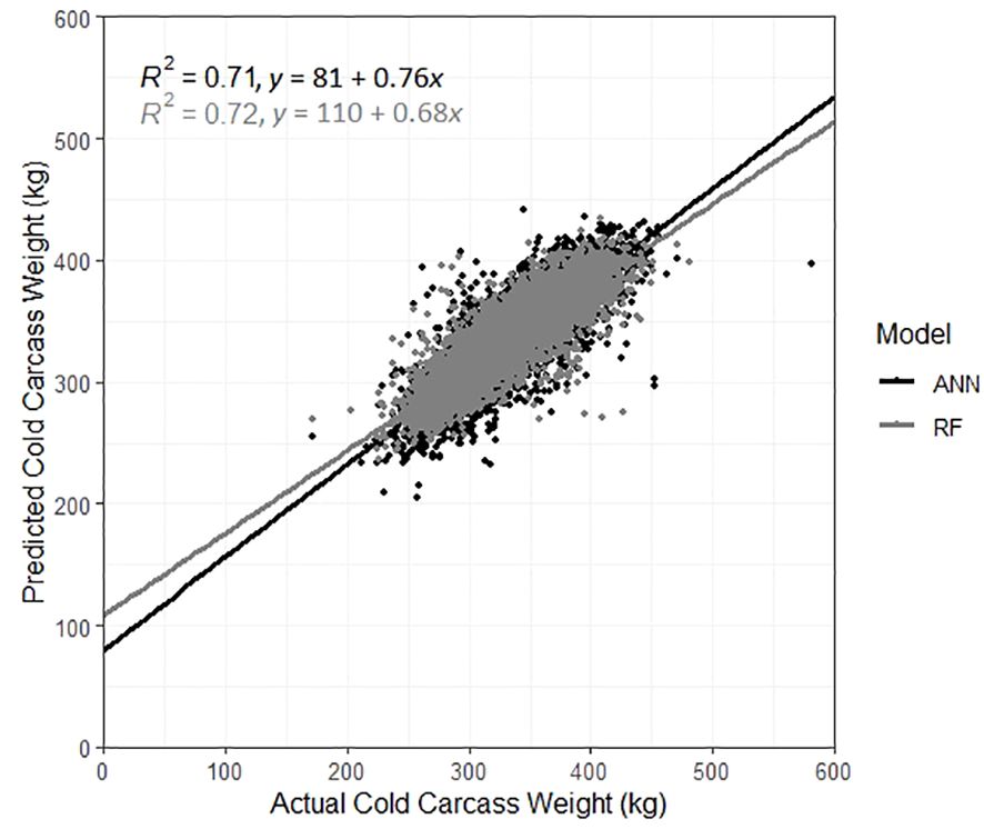
Figure 3 Actual vs. predicted cold carcass weight for carcasses in the validation dataset, predicted using the best artificial neural network model (black) and the best random forest model (grey).

Table 4

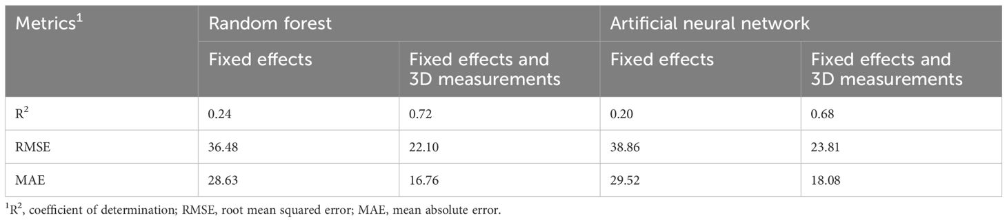
Table 4 Comparison of results for different metrics across the best random forest model and best artificial neural network model for the prediction of cold carcass weight, considering only fixed effects (kill date, sex and breed type), and fixed effects and 3D measurements.

Table 5

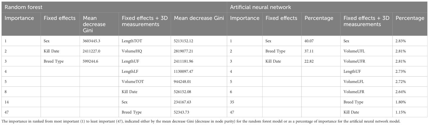
Table 5 Importance of variables in the best random forest model and artificial neural network model, built for the prediction of cold carcass weight.

Artificial neural networks

The R² values for the ANNs built using only fixed effects (n = 12) ranged between 0.16–0.20. The RMSE for the ANNs ranged between 36.84–38.86kg and the MAE ranged between 29.52–31.50. The RMSE was used to select the optimal model, and this was identified as the model built with a size of 6 and decay of 0.01. The sex of the carcass was identified as the most important variable (40.07%), followed by breed type (37.11%) and then kill date (22.82%).

When including the dimensional measurements, both RMSE and MAE decreased, and the R² increased across all size and decay combinations (n = 12). The R² ranged from 0.58–0.68 and the MAE ranged from 18.08–20.10. The RMSE ranged from 23.81–28.02kg, with the lowest RMSE resulting from the model built with a size of 40 and a decay of 0.001. This model was then used to predict the CCW of carcasses in the validation dataset. The actual and predicted weights are displayed in Figure 3, with the best fit line (y = 81 + 0.76x).

Results from the most accurate ANN models built for the prediction of CCW are displayed in Table 4 and the top 5 most important 3D measurements included in those models, along with the ranking of the fixed effects importance are listed in Table 5. When including the 3D measurements in the ANN models, the most important variable was again identified as sex (2.83%). The breed type was the 39th most important variable (1.80%) and the kill date was the least important (1.15%). The volume of the upper flank (VolUF) was the second most important variable and the most important 3D measurement in the ANN.

Prediction of conformation class

Random forests

A total of 520 RF models were built for the prediction of conformation class. Of the 40 RFs built using fixed effects only, the accuracy ranged between 0.59–0.65. The most accurate RF consisted of 900 trees and a mtry of 2, with an OOB estimate of error of 35.22%. The model predicted 69% of the training dataset’s classes correctly and a further 29% were over-/underscored by only one neighboring grade. Slightly lower results were seen for the validation dataset, however, where the model predicted 64% of classes correctly and 34% of classes were over-/under-scored by one.

For the final model built using only fixed effects, CCW was found to be the most important variable. Kill date and breed type were the two next most important variables, with sex being the least important variable in the model. Random forests built including the dimensional measurements resulted in more accurate models, with accuracy ranging between 0.63–0.71. Of the 480 RF models built including the 3D measurements, the most accurate model was built with 900 trees and 32 variables at each split with an OOB estimate of error rate of 29.24%. This RF predicted 100% of classes correctly in the training dataset. The confusion matrix built using the validation dataset (Table 6) showed that 71% of classes were correctly classified (black) and 28% were over/under-scored by one neighboring class (grey).

Table 6

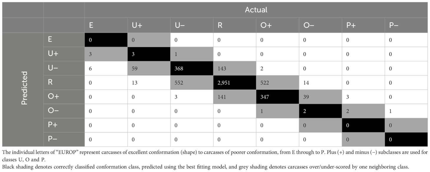
Table 6 Confusion matrix for actual vs. predicted conformation classes for carcasses in the validation dataset, predicted using the best random forest model built using fixed effects and 3D measurements.

For the most accurate model including the 3D measurements, CCW was again the most important variable. The width of the forequarter, the total length of the carcass and the width of the flank were identified as the top three most important measurements after CCW. Kill date was identified as the sixth most important variable and breed type as the eight. The sex of the carcass was again identified as the least important variable. Results from the most accurate RF models for the prediction of conformation class are displayed in Table 7 and the top 5 most important 3D measurements in those models, along with the ranking of the fixed effects importance, are listed in Table 8.

Table 7

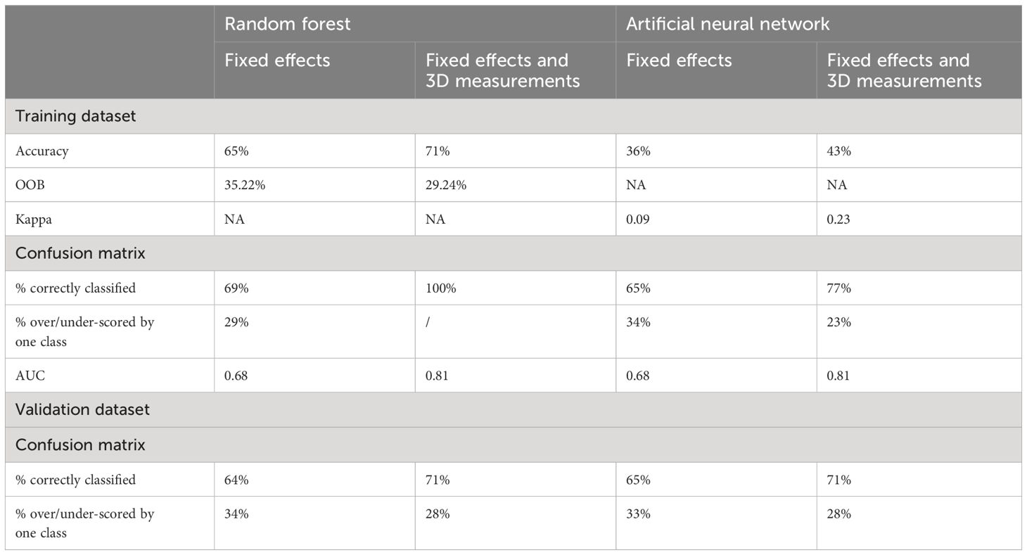
Table 7 Comparison of results for different metrics across the best random forest model and best artificial neural network model for the prediction of conformation class, considering only fixed effects (kill date, sex, breed type and CCW), and fixed effects and 3D measurements.

Table 8

Table 8 Importance of variables in the best random forest model and artificial neural network model, built for the prediction of conformation class.

Artificial neural networks

A total of 24 ANN models were built for the prediction of conformation class. All twelve ANN models built using only fixed effects resulted in accuracies of 36% and the Kappa statistic ranged between 0.08–0.09. The most accurate model had a size of 6 and a decay of 0.001. The confusion matrix resulted in an accuracy of 65% for both the predicted classes in the training dataset and validation dataset. A further 34% of classes for the training dataset and 33% in the validation dataset were over-/under-scored by one class. The averaged multiclass AUC for this best model, built using only fixed effects was 0.68. The most important variable for the prediction of conformation class, using the best ANN with only fixed effects was identified as the sex of the carcass (33.85%). The breed type (31.19%) and CCW (23.73%) were the second and third most important variables respectively, and the kill date was the least important variable in the ANN (11.23%).

Including the 3D measurements in the models improved accuracies, with 41–43% of classes being classified correctly across the 12 models, and the Kappa statistic increased, ranging between 0.18–0.23. The optimal model was built with a size of 20 and a decay of 0. The confusion matrix for the training dataset showed that the model predicted 77% of classes correctly and 23% were over-/under-scored by one class. For the validation dataset (Table 9) the confusion matrix showed 71% of classes were predicted correctly (black) using the best model. A further 28% were classified within the neighboring class (grey). The averaged AUC across the classes was 0.81. The CCW was identified as the most important variable in the best ANN using fixed effects and 3D measurements (6.33%). The sex (3.09%) and the breed type (3.09%) were the third and fourth most important variables. The kill date was the 26th most important variable (1.81%) out of the 48 variables input into the model. LenTOT was the second most important variable (3.31%) and the most important 3D measurement.

Table 9

Table 9 Confusion matrix for actual vs. predicted conformation classes for carcasses in the validation dataset, predicted using the best artificial neural network.

Prediction of fat class

Random forests

For the 520 RFs built for the prediction of fat classification, again 40 of those were built using only fixed effects, with the mtry ranging between 1–4. The percentage of correctly classified classes resulting from the models ranged between 46–55%. The RF identified as the best model included 500 trees and a mtry of 2. The OOB estimate of error rate for this model was 45.47%. The model predicted 56% of classes in the training dataset correctly and a further 39% of classes were over/under-scored by one neighboring class. Similar results were seen for the validation dataset, where the model predicted 55% of classes correctly and 40% within one neighboring class. The averaged multiclass AUC for fat classes predicted using the best RF with the fixed effects only, was 0.58. The CWW was the most important variable in the best RF model build including only fixed effects, followed by kill date, breed type and finally the sex of the carcass.

The remaining 480 RFs, using fixed effects plus dimensional measurements, combining the ntree values with the mtry values (1:48) resulted in similar accuracies however, ranging from 0.54–0.56. The best model had 1,000 trees and a mtry of 33 and an OOB estimate of error rate of 44.24%. When the model was used to predict the fat class of carcasses in the training dataset, 100% of classes were predicted correctly. When used to predict unseen data from the validation dataset (Table 10), the model predicted 57% of fat classes correctly (black), and a further 28% were over/under-scored by one subclass (grey).

Table 10

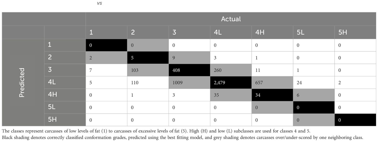
Table 10 Confusion matrix of actual vs. predicted fat classes for carcasses in the validation dataset, predicted using the best random forest.

The CCW was identified as the most important variable in this RF. Kill date was the second most important variable, however the breed type and the sex of the carcass were the 47th and 48th most important variables respectively. Width of the flank (WidthF) was the third most important variable in the RF. The averaged area under the multiclass curve was 0.69.

Results from the most accurate RF models for the prediction of fat class are displayed in Table 11 and the top 5 most important 3D measurements in those models, along with the ranking of the fixed effects importance, are listed in Table 12.

Table 11

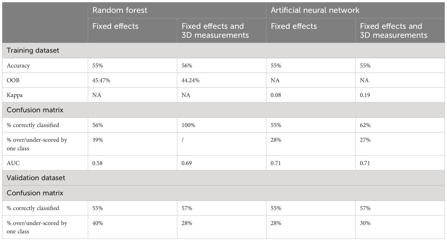
Table 11 Comparison of results for different metrics across the best random forest model and best artificial neural network model for the prediction of fat class, considering only fixed effects (kill date, sex, breed type and CCW), and fixed effects and 3D measurements.

Table 12

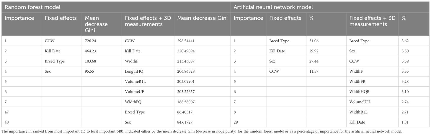
Table 12 Importance of variables in the best random forest model and artificial neural network model, built for the prediction of fat class.

Artificial neural networks

The accuracy for all 12 ANNs built for the prediction of fat class, using fixed effects, was 0.55 and the Kappa statistic was 0.08. The best model was defined as the model built with a size of 4 and a weight decay of 0. The confusion matrices for both the training and validation dataset produced the same results, with 55% of fat classes predicted correctly, and 28% within one neighboring class. The averaged multiclass AUC was 0.71. Breed type was identified as the most important variable (31.06%), followed by kill date (29.92%), sex (27.44%) and finally CCW (11.57%).

The ANNs for prediction of fat class including the dimensional measurements (n = 12) resulted in accuracies of 0.48–0.54. The Kappa ranged between 0.15–0.19. The best model was defined as the ANN with size = 20 and decay = 0. The best model predicted 62% of classes correctly with the training dataset and 27% within one neighboring class. The confusion matrix comparing actual and predicted fat classes for carcasses in the validation dataset, predicted using the best ANN (Table 13) showed 57% of classes were correctly predicted (black) and 30% were classified within one neighboring class (grey). The averaged AUC across the classes was 0.77. The breed type of the carcass was again identified as the most important variable (3.62%) for the prediction of carcass fat class. Sex (3.50%) and CCW (3.39%) were the second and third most important variables, followed by WidFL (width of the flank to the left of the axis), which was the most important 3D measurement (3.35%). Kill date was the 29th most important variable in the best ANN (1.81%).

Table 13

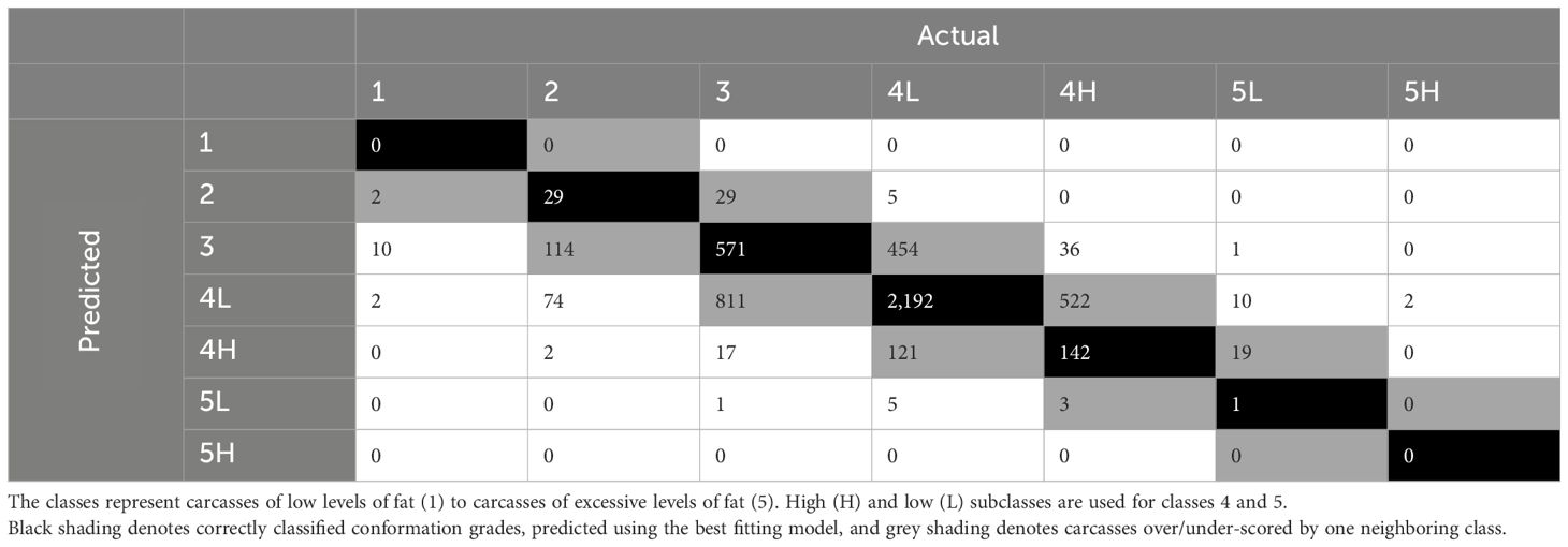
Table 13 Confusion matrix for actual vs. predicted fat classes for carcasses in the validation dataset, predicted using the best artificial neural network.

Results from the most accurate artificial neural network models for the prediction of fat class are displayed in Table 11 and the top 5 most important 3D measurements in those models, along with the ranking of the fixed effects importance, are listed in Table 12.

Discussion

Supervised machine learning algorithms (random forests and artificial neural networks) were used to predict the conformation class, fat class, and CCW of beef carcasses. The models were built using either fixed effects or fixed effects and 3D measurements (widths, lengths and volumes) extracted from 3D images of the carcasses. The study aimed not only to compare the prediction accuracies resulting from the two machine learning techniques, but also the accuracies resulting from the two sets of variables.

Prediction of cold carcass weight

Machine learning models built for the prediction of CCW using fixed effects only resulted in low accuracies (R²). The best RF resulted in higher accuracies than that of the best ANN, however, with an increase from 0.20 to 0.24. These results were similar to those achieved using traditional statistics (multiple linear regression) with the same dataset, where the R² = 0.22 (Nisbet et al., 2024). In terms of all models built using only fixed effects, the accuracies (R²) for CCW were lowest across the three traits. This could be due to the other traits including an additional fixed effect predictor (CCW), which may have a stronger relationship with the other two traits compared to the breed, sex and kill date alone. This can be seen with the models for fat and conformation, where the CCW was in the top three most important variables across both methods per trait, including or excluding the 3D measurements.

In terms of the variables highlighted as important for the prediction of CCW, there were few similarities across the two machine learning methods. For models built including only the fixed effects, sex was the most important variable, and this was also the most important variable in the ANN build including the 3D measurements suggesting differences in the carcass weight of steer and heifer carcasses. This agrees with that of previous studies, where significant differences have been noted between the sex of a carcass and the carcass weight (Tůmová et al., 2021). Heggli et al. (2021) also found carcass weights between young bulls and heifers to be significantly different.

Despite this, in the current study, sex was, however, the 14^th most important predictor in the RF model, and placed after kill date, which was second in the RF model built including only fixed effects. The remaining fixed effects were found to have little importance when predicting CCW, indicating the 3D measurements to be valuable in the prediction of this trait. In particular, the measurements from the upper flank section of the carcass (VolumeUFL, VolumeUFR, and LengthUF) were identified as important for the prediction of CCW, being the 2^nd–4^th most important variables in the ANN, and the LengthUF was the third most important variable in the RF model. The total length of the carcass was the most important variable in the RF model. This may be explained by the fact that CCW and the total length of the carcass (LenTOT) were highly correlated (R² = 0.69), mirroring that of a study by Seo et al. (2021), where the carcass weight and total length of the carcass were found to be highly correlated. In the current study, kill date was the 8^th most important, sex was the 14^th most important, and breed type was the least important variable. For the ANNs, however, breed type and kill date were the second least and least important variables respectively. This further indicates the weak relationship between the fixed effects and the cold weight of the carcass, and hence the importance of dimensional measurements for CCW prediction.

Including the dimensional measurements in the models increased accuracies compared to that of models built just including fixed effects for both machine learning techniques (RF R² = 72%; ANN R² = 68%). The results using the machine learning approaches were similar to those previously obtained from the same dataset using traditional statistics (multiple linear regression) (Nisbet et al., 2024), where the prediction accuracy again improved when including the 3D measurements (R² = 0.70). Although the previously fitted linear regression models resulted in higher accuracies than that of the ANNs, the RF models outperformed all tested techniques. This is similar to results found in a study by Shahinfar et al. (2019), where RFs resulted in higher accuracies than that of linear regression models for the prediction of all tested carcass traits. For the prediction of hot carcass weight in particular, the linear regression models resulted in correlation coefficients of 0.68, whereas the RF models resulted in a correlation coefficient of 0.79, despite linear regression being viewed as the “gold standard”. There are many potential reasons why the RF model may have outperformed the linear regression models, one of which being the fact RFs are ensemble approaches, allowing them to overcome limitations such as overfitting (Chiaverini et al., 2023). In order to avoid overfitting with linear regression, typically variables included in models have to meet a certain criterion and thus are user chosen. This was also the case in the previous study (Nisbet et al., 2024) due to the stepwise selection method, and variance inflation factor threshold (<5). Machine learning approaches, however, are data driven and thus the model is created by the algorithm based on the available data. Therefore, machine learning techniques are often superior to traditional methods such as linear regression, particularly when many variables are included (Ley et al., 2022). The parameter tuning implemented for the RF algorithms also may have aided this, with every possible number of variables being tested at each split, across different RFs resulting in 470 different parameter combinations. This allowed for an optimum variable input number to be highlighted, and although this was not always the maximum possible, it did not mean any variables were necessarily excluded from the random forest. This, along with the utilization of bagging (bootstrap aggregation), which seems to enhance accuracy (Breiman, 2001), may also provide an explanation as to why the RFs outperformed the results produced from the ANN models, which had no form of feature selection or refinement of included variables, which may have lead to the inferior results, compared to the two other tested techniques. Similarly, it has also been noted that RF models perform better on medium sized datasets than ANN algorithms (Grinsztajn et al., 2022), suggesting the RF algorithms are more suited to the current dataset compared to that of the ANNs algorithms.

the results in the current study were lower than those reported by Alves et al. (2019), where measurements were used to predict the hot carcass weight of commercial lambs with high accuracy(R² = 0.82 when considering all variables, or R² = 0.88 when using variable selection methods). These measurements, however, were recorded directly on the live animal, rather than on images of the carcass, and included physical measurements as well as subjective scores. Similar accuracies to Alves et al. (2019) have been found in a study by Miller et al. (2019), where a series of measurements from 3D images of live beef animals were used to predict the CCW, using either traditional statistics or machine learning approaches. The machine learning techniques (ANNs) resulted in R² of 0.88, higher than that of the results from the multiple linear regression models (R² = 0.83), again built using stepwise selection methods. Both, however, were higher than that of the current study. Miller et al. (2019) included height measurements of the live animal, which may offer an insight into the volume of the carcass and, therefore, its potential weight. Depth measurements of the carcass were not measured in the current study, however, the 3D volumes were used to convey the depth of the carcass. Although the measurements are only extracted from one half of the carcass (right hand side), they are used to predict the combined weight of both sides. Differences in the two sides, as a result of dressing for example, could impact the accuracy of the prediction.

Prediction of conformation class

Including the dimensional measurements in the models resulted in increased prediction accuracies for both the RFs and the ANNs (7% increase across both methods). Although the percentage increase was similar across the two traits, the RF algorithm resulted in higher accuracies than that of the ANN models, for both predictions made using fixed effects only, and fixed effects and 3D measurements.

Despite the 3D measurements adding value in terms of increasing the prediction accuracies, the CCW was identified as the most important variable across both techniques for models built including the dimensional measurements, indicating the role the fixed effects still play in the accuracy. This can further be seen in the ANN, where sex and breed type were both included in the top 5 most important variables. Despite this, the sex was listed as the least important variable for both RF models and the kill date was the 6^th most important variable in the RF model, however the 28^th most important variable in the ANN. The total length of the carcass (LengthTOT) was ranked in the top 3 most important variables for both techniques, suggesting this measurement has a strong relationship with the conformation. The total volume of the carcass, however, was not highly ranked (top 5) in either model, which was suspected to have a strong relationship with the conformation.

The results recorded were slightly higher than those produced from the same dataset using traditional statistics (multiple linear regression), rather than machine learning techniques (Nisbet et al., 2024). The stepwise selection models in that previous study built using only fixed effects resulted in low accuracy for the prediction of conformation class (R² = 0.22, RMSE = 36.48kg). The accuracy increased, however, when the same set of 3-dimensional measurements were included in the models (R² = 0.48, RMSE=0.99). Despite this, the prediction accuracies for both machines learning techniques, using either fixed effects (64–65%) or fixed effects and 3D measurements (71%) were higher than the accuracies resulting from the respective multiple linear regression models. This is also consistent with findings by Díez et al. (2003) where three separate machine learning techniques outperformed linear regression models when being used for the prediction of conformation class, in terms of resulting in lower errors. This may be due to the potential for machine learning algorithms to specify whether an output is linear or categorical. Despite this, in a study by Díez et al. (2006), the machine learning technique used to predict conformation was found to mimic that of the linear regression model that was also performed in the study.

In the current study, only carcass categories steer and heifer were included, limiting the age range of the carcasses, with young or older animals being excluded from the dataset. It was noted by Díez et al. (2006), however, that there is a strong relationship between age and conformation. The current study only included data from carcasses of steers (castrated male animal aged from 12 months) and heifers (female animal aged from 12 months that has not calved). Therefore, young animals (<12 months of age) were not included, reducing the variety of ages seen in the study. Further to this, it is also unlikely that older animals were present in the study, due to the nature of beef enterprises in the UK, (castrated males are scarcely kept for longer than a few years, and female cattle over 2 years would typically have calved and, therefore, no longer be classified as a heifer). Therefore, this suggest the cattle in the current study are likely to be aged between one and two years of age, leading to a lack of variation in the current study that could bias the results.

Prediction of fat class

The best random forests and artificial neural network models resulted in moderate accuracy for the prediction of fat class. Including the dimensional measurements only increased accuracy for the RF models, increasing accuracy from 55% to 56%. The ANN model accuracies did not change (55%) when the 3D measurements were included. When using the models to predict the fat classes of carcasses in the validation dataset, however, the model including the dimensional measurements resulted in increased accuracies across both techniques, albeit by only by 2%. Similar results were seen in a study by Miller et al. (2019), where ANN built using measurements from 3D images of live animals predicted the fat class of beef carcasses with 54.2% accuracy. The lack of increase in the prediction accuracy when including the measurements in the current study, however, suggests that the 3D measurements do not add any predictive power to the models. Despite this, prediction accuracies were still greater than those produced using linear regression models (Nisbet et al., 2024), which produced low accuracies for both the models built, using only fixed effects (R² = 0.12) and including the 3D measurements (R² = 0.20). The machine learning techniques may have outperformed the linear regression models due to the trait being categorical, and therefore less suited to linear methods than that of machine learning. This may have allowed for the RF models and ANN models to result in more accurate outcomes with little information compared to that of the linear regression models in the previous study, particularly for the models built using only fixed effects. The minimal increase in prediction accuracy resulting from the inclusion of the 3D measurements in the models, however, was anticipated as it has been recognized previously that the fat class of a carcass has little relationship with the conformation (shape) of a carcass For example the two traits were found to have a low correlation (r = 0.07) in a study by Conroy et al. (2010). The 3D measurements were further found to add little value in terms of the ranking of importance, with the most important variable in both models built including 3D measurements being one of the fixed effects. For the RF model, the top 3 most important variables were all fixed effects (breed type, sex and CCW). The CCW was the most important variable in the ANN model, however, breed type and sex were found to be least important, ranking 47^th and 48^th respectively, showing inconsistencies in the role the fixed effects play across the techniques. The width of the flank (WidthF) was the most important 3D measurement in both the RF and ANN algorithms (ranked 4^th and 3^rd respectively), however, showing consistencies with the 3D measurements and their importance.

As the 3D measurements were highlighted as less important for the prediction of fat class, and negligible improvements were observed in the accuracies between models built including the 3D measurements and models built using only the fixed effects, it can therefore be understood why many alternative technologies rely on color scales for the prediction of fat class, over carcass measurements that are otherwise extracted for the prediction of conformation class. The BCC-2 has used color data extracted from carcasses to build linear models, predicting the fat class with high accuracy (R² = 0.75) (Borggaard et al., 1996). The same technology has also been compared with two other VIA systems using color scales for classification (VIAscan^® and VBS2000), and their ability to predict carcass grades assigned by a reference panel (Allen and Finnerty, 2000). All three technologies, however, predicted fat class on the 15-point scale with low accuracy, classifying 28.0–34.4% of fat classes correctly. The accuracies were higher, however, when predicting on a smaller scale (5-point scale), predicting fat class with 66.8–72.2% accuracy. Predicting on a smaller fat class scale outperforms the prediction on the 15-point scale, perhaps indicating why the results of the current study (estimating on an 8-point scale) resulted in higher accuracies using the carcass measurements than Allen and Finnerty’s 15-point scale color data results, using color data. Despite the benefits that may result from using color scales, there is still the question as to whether the extracted measurements are indeed representative of the key areas to assess when predicting the carcass traits. Although the measurements were based on literature searches and expert opinion, alternative methods for estimating the traits and selecting predictors may also be useful, such as using the raw image to predict the carcass traits, rather than using the extracted measurements. This has the potential to be achieved using deep learning, and further studies are warranted to assess the potential of this. Alternatively, it is also worth considering whether the assessed categorical traits are the best traits to be used for determining the value of a carcass. Alternative characteristics, such as the saleable meat yield of a carcass, may offer more insight into the true value of a carcass. In a study by Allen and Finnerty (2000), the first of two trials compared three video image analysis systems and their ability to predict beef carcass conformation class, fat class, and saleable meat yield. The trial found the systems to be accurate in predicting the saleable meat yield, indicating the potential for video image analysis systems to be used for estimating alternative carcass traits, which may offer a more accurate and true representation of the value of a carcass.

Conclusion

This study explored the use of machine learning techniques (random forests and artificial neural networks) and their ability to predict carcass classification grades and carcass weight, using a series of 3D measurements, extracted using a new imaging system that required limited infrastructure. Initially models were built using only fixed effects, excluding the 3D measurements. These models indicated the predictive power of these variables alone, and in turn indicated the added value resulting from including the measurements in further models. The prediction accuracy increased across all traits when the dimensional measurements were included, with the exception of the artificial neural networks built for the prediction of fat class. The study confirmed previous findings suggesting the potential for the 3D measurements and the camera system to predict key carcass traits. Along with this, it indicated that the machine learning techniques provide a promising avenue forward to predict carcass weight and conformation. However, further improvement for predicting fat content may be expected by including color scales in the image data.

Data availability statement

The data analyzed in this study is subject to the following licenses/restrictions: Private Data. Requests to access these datasets should be directed to Holly Nisbet, holly.nisbet@sruc.ac.uk.

Author contributions

HN: Conceptualization, Formal analysis, Methodology, Writing – original draft. NL: Conceptualization, Methodology, Supervision, Writing – review & editing. GM: Conceptualization, Methodology, Supervision, Writing – review & editing. AD-W: Supervision, Writing – review & editing. DB: Data curation, Investigation, Resources, Software, Writing – review & editing. AW: Data curation, Investigation, Resources, Software, Writing – review & editing. C-AD: Conceptualization, Funding acquisition, Methodology, Supervision, Writing – review & editing.

Funding

The author(s) declare financial support was received for the research, authorship, and/or publication of this article. The authors acknowledge Scotland’s Rural College (SRUC) and the Agricultural and Horticultural Development Board (AHDB) for funding the study. Innovent Technology Ltd. for creating the technology and processing the images. The AD-W contribution was funded by the BBSRC Institute Strategic Program Grants BBS/E/RL/230001C and BBS/E/RL/230002D. The data collected for this study was funded UKRI Innovate UK through the OPTI-BEEF project (ref. 105146).

Conflict of interest

Authors DB and AW were employed by the company InnoventTechnology Ltd.

The remaining authors declare that the research was conducted in the absence of any commercial or financial relationships that could be construed as a potential conflict of interest.

Publisher’s note

All claims expressed in this article are solely those of the authors and do not necessarily represent those of their affiliated organizations, or those of the publisher, the editors and the reviewers. Any product that may be evaluated in this article, or claim that may be made by its manufacturer, is not guaranteed or endorsed by the publisher.

References

AHDB. (2024). Using the EUROP grid in beef carcase classification. Available online at: https://ahdb.org.uk/knowledge-library/using-the-europ-grid-in-beef-carcase-classification (Accessed February 2, 2024).

Google Scholar

Allen P., Finnerty N. (2000). Objective beef carcass classification. A report of a trial of three VIA classification systems. Dublin, Ireland: The Department of Agriculture, Food and Rural Development, and the National Food Centre, Teagasc.

Google Scholar

Alves A. A. C., Chaparro Pinzon A., da Costa R. M., da Silva M. S., Vieira E. H. M., de Mendonça I. B., et al. (2019). Multiple regression and machine learning based methods for carcass traits and saleable meat cuts prediction using non-invasive in vivo measurements in commercial lambs. Small Ruminant Res. 171, 49–56. doi: 10.1016/j.smallrumres.2018.12.008

CrossRef Full Text | Google Scholar

Benos L., Tagarakis A. C., Dolias G., Berruto R., Kateris D., Bochtis D. (2021). Machine learning in agriculture: A comprehensive updated review. Sensors 21. doi: 10.3390/s21113758

PubMed Abstract | CrossRef Full Text | Google Scholar

Borggaard C., Madsen N. T., Thodberg H. H. (1996). In-line image analysis in the slaughter industry, illustrated by Beef Carcass Classification. Meat Sci. 43, 151–163. doi: 10.1016/0309-1740(96)00062-9

CrossRef Full Text | Google Scholar

Bozkurt Y., Aktan S., Ozkaya S. (2008). Digital image analysis to predict carcass weight and some carcass characteristics of beef cattle. Asian J. Anim. Veterinary Adv. 3, 129–137. doi: 10.3923/ajava.2008.129.137

CrossRef Full Text | Google Scholar

Breiman L. (2001). Random forests. Mach. Learn. 45, 5–32. doi: 10.1023/A:1010933404324

CrossRef Full Text | Google Scholar

British Cattle Movement Service. (2014). Official cattle breeds and codes. Available at: https://www.gov.uk/guidance/official-cattle-breeds-and-codes (Accessed 13 April 2023).

Google Scholar

Bzdok D., Altman N., Krzywinski M. (2018). Statistics versus machine learning. Nat. Methods 15, 233–234. doi: 10.1038/nmeth.4642

PubMed Abstract | CrossRef Full Text | Google Scholar

Chiaverini L., Macdonald D. W., Hearn A. J., Kaszta Ż., Ash E., Bothwell H. M., et al. (2023). Not seeing the forest for the trees: Generalised linear model out-performs random forest in species distribution modelling for Southeast Asian felids. Ecol. Inf. 75, 102026. doi: 10.1016/j.ecoinf.2023.102026

CrossRef Full Text | Google Scholar

Conroy S. B., Drennan M. J., McGee M., Keane M. G., Kenny D. A., Berry D. P. (2010). Predicting beef carcass meat, fat and bone proportions from carcass conformation and fat scores or hindquarter dissection. Animal 4, 234–241. doi: 10.1017/S1751731109991121

PubMed Abstract | CrossRef Full Text | Google Scholar

Craigie C. R., Navajas E. A., Purchas R. W., Maltin C. A., Bünger L., Hoskin S. O., et al. (2012). A review of the development and use of video image analysis (VIA) for beef carcass evaluation as an alternative to the current EUROP system and other subjective systems. Meat Sci. 92, 307–318. doi: 10.1016/j.meatsci.2012.05.028

PubMed Abstract | CrossRef Full Text | Google Scholar

De La Iglesia D. H., González G. V., García M. V., Rivero A. J. L., De Paz J. F. (2020). Non-invasive automatic beef carcass classification based on sensor network and image analysis. Future Generation Comput. Syst. 113, 318–328. doi: 10.1016/j.future.2020.06.055

CrossRef Full Text | Google Scholar

Díez J., Albertí P., Ripoll G., Lahoz F., Fernández I., Olleta J. L., et al. (2006). Using machine learning procedures to ascertain the influence of beef carcass profiles on carcass conformation scores. Meat Sci. 73, 109–115. doi: 10.1016/j.meatsci.2005.11.015

PubMed Abstract | CrossRef Full Text | Google Scholar

Díez J., Bahamonde A., Alonso J., López S., Del Coz J. J., Quevedo J. R., et al. (2003). Artificial intelligence techniques point out differences in classification performance between light and standard bovine carcasses. Meat Sci. 64, 249–258. doi: 10.1016/S0309-1740(02)00185-7

PubMed Abstract | CrossRef Full Text | Google Scholar

Emenheiser J. C., Greiner S. P., Lewis R. M., Notter D. R. (2010). Validation of live animal ultrasonic measurements of body composition in market lambs. J. Anim. Sci. 88, 2932–2939. doi: 10.2527/jas.2009-2661

PubMed Abstract | CrossRef Full Text | Google Scholar

Goyache F., Bahamonde A., Alonso J., Lopez S., Del Coz J. J., Quevedo J. R., et al. (2001). The usefulness of artificial intelligence techniques to assess subjective quality of products in the food industry. Trends Food Sci. Technol. 12, 370–381. doi: 10.1016/S0924-2244(02)00010-9

CrossRef Full Text | Google Scholar

Grinsztajn L., Oyallon E., Varoquaux G. (2022). Why do tree-based models still outperform deep learning on tabular data? Adv. Neural Inf. Process Syst. doi: 10.48550/ARXIV.2207.08815

CrossRef Full Text | Google Scholar

Hansard M., Lee S., Choi O., Horaud R. (2013). Time-of-flight Cameras: Principles, Methods and Applications (London: Springer London (SpringerBriefs in Computer Science). doi: 10.1007/978-1-4471-4658-2

CrossRef Full Text | Google Scholar

Heggli A., Gangsei L. E., Røe M., Alvseike O., Vinje H. (2021). Objective carcass grading for bovine animals based on carcass length. Acta Agriculturae Scandinavica A: Anim. Sci. 70, 113–121. doi: 10.1080/09064702.2021.1906940

CrossRef Full Text | Google Scholar

Kuhn M. (2008). Building predictive models in R using the caret package. J. Stat. Software 28. doi: 10.18637/jss.v028.i05

CrossRef Full Text | Google Scholar

Ley C., Martin R. K., Pareek A., Groll A., Seil R., Tischer T. (2022). Machine learning and conventional statistics: making sense of the differences. Knee Surgery Sports Traumatology Arthroscopy 30, 753–757. doi: 10.1007/s00167-022-06896-6

CrossRef Full Text | Google Scholar

Liakos K., Busato P., Moshou D., Pearson S., Bochtis D. (2018). Machine learning in agriculture: A review. Sensors 18, 2674. doi: 10.3390/s18082674

PubMed Abstract | CrossRef Full Text | Google Scholar

Miller G. A., Hyslop J. J., Barclay D., Edwards A., Thomson W., Duthie C. A. (2019). Using 3D imaging and machine learning to predict liveweight and carcass characteristics of live finishing beef cattle. Front. Sustain. Food Syst. 3. doi: 10.3389/fsufs.2019.00030

CrossRef Full Text | Google Scholar

Nisbet H., Lambe N., Miller G., Doeschl-Wilson A., Barclay D., Wheaton A., et al. (2024). Using in-abattoir 3-dimensional measurements from images of beef carcasses for the prediction of EUROP classification grade and carcass weight. Meat Sci. 209, 109391. doi: 10.1016/j.meatsci.2023.109391

PubMed Abstract | CrossRef Full Text | Google Scholar

R Core Team. (2023). R: a language and environment for statistical computing. Vienna, Austria: R Foundation for Statistical Computing. Available at: https://www.R-project.org/.

Google Scholar

Rius-Vilarrasa E., Bünger L., Maltin C., Matthews K. R., Roehe R. (2009). Evaluation of Video Image Analysis (VIA) technology to predict meat yield of sheep carcasses on-line under UK abattoir conditions. Meat Sci. 82, 94–100. doi: 10.1016/j.meatsci.2008.12.009

PubMed Abstract | CrossRef Full Text | Google Scholar

Robin X., Turck N., Hainard A., Tiberti N., Lisacek F., Sanchez J.-C., et al. (2011). pROC: an open-source package for R and S+ to analyze and compare ROC curves. BMC Bioinf. 12, 77. doi: 10.1186/1471-2105-12-77

CrossRef Full Text | Google Scholar

Seo H.-W., Ba H. V., Seong P.-N., Kim Y.-S., Kang S.-M., Seol K.-H., et al. (2021). Relationship between body size traits and carcass traits with primal cuts yields in Hanwoo steers. Anim. Bioscience 34, 127–133. doi: 10.5713/ajas.19.0809

CrossRef Full Text | Google Scholar

Shahinfar S., Kelman K., Kahn L. (2019). Prediction of sheep carcass traits from early-life records using machine learning. Comput. Electron. Agric. 156, 159–177. doi: 10.1016/j.compag.2018.11.021

CrossRef Full Text | Google Scholar

Stinga L., Bozzo G., Ficco G., Savarino A. E., Barrasso R., Negretti P., et al. (2020). Classification of bovine carcasses: New biometric remote sensing tools. Ital. J. Food Saf. 9, 93–97. doi: 10.4081/ijfs.2020.8645

CrossRef Full Text | Google Scholar

Strydom P. E. (2022). Classification of carcasses | beef carcass classification and grading. Encyclopedia Meat Sci. (Third edition), 688–709. doi: 10.1016/B978-0-323-85125-1.00014-4

CrossRef Full Text | Google Scholar

Tůmová E., Chodová D., Volek Z., Ketta M. (2021). The effect of feed restriction, sex and age on the carcass composition and meat quality of nutrias (Myocastor coypus). Meat Sci. 182, 108625. doi: 10.1016/j.meatsci.2021.108625

PubMed Abstract | CrossRef Full Text | Google Scholar

Venables W. N., Ripley B. D., Venables W. N. (2002). Modern applied statistics with S. 4th ed (New York: Springer (Statistics and computing).

Google Scholar

Wnęk K., Gołębiewski M., Przysucha T. (2017). Validation of the first objective evaluation system for beef carcasses. Can. J. Anim. Sci. 98, 53–60. doi: 10.1139/CJAS-2016-0241

CrossRef Full Text | Google Scholar