Enhancing constituent estimation in nucleic acid mixture models using spectral annealing inference and MS/MS information

Mass spectrometry (MS) is a powerful analytical technique employed for a variety of applications including drug development, quality assurance, food inspection, and monitoring environmental pollutants. Recently, in the production of actively developed antibody and nucleic acid pharmaceuticals, impurities with various modifications have been generated. These impurities can lead to a decrease in drug stability, pharmacokinetics, and efficacy, making it crucial to distinguish between them. We previously modeled mass spectrometry for each possible number of constituents in a sample, using parameters such as monoisotopic mass and ion counts, and employed stochastic variational inference to determine the optimal parameters and the maximum posterior probability for each model. By comparing the maximum posterior probabilities among models, we selected the optimal number of constituents and inferred their corresponding monoisotopic masses and ion counts. However, MS spectra are sparse and predominantly flat, which can lead to vanishing gradients when using simple optimization techniques. To solve this problem, using MCMC as in our previous studies would take a very long time. To address this difficulty, in this study, we blur the comparative spectra and gradually reduce the blur to prevent vanishing gradients while inferring accurate values. Furthermore, we incorporate MS/MS spectra into the model to increase the amount of information available for inference, thereby improving the accuracy of parameter inference. This modification improved the mass error from an average of 1.348 Da–0.282 Da. Moreover, the required time, even including the processing of additional five MS/MS spectra, was reduced to less than half.

1 Introduction

Mass Spectrometry (MS) serves as a robust analytical method and is employed across various fields including drug development, food safety inspections, and environmental pollutant monitoring. In recent years, with the vigorous development of antibodies and nucleic acid drugs, impurities with different modifications have been produced. Such impurities may adversely affect the stability, pharmacokinetics, and efficacy of drugs (Sanghvi, 2011; Weinberg et al., 2005; Tamara, den Boer, and Heck, 2022; Pecori et al., 2022). It is, therefore, essential in pharmaceutical development and quality control to identify and address these multiple impurities. Additionally, understanding the monoisotopic mass of the constituents can offer crucial insights into the origins of impurity formation. Similarly, knowledge of the ion concentrations of these constituents assists in evaluating the potential impact of the impurities.

In contemporary mass spectrometry, accurately identifying impurities in middle or high molecules with minor modifications remains challenging. Traditional chromatography methods frequently struggle to effectively separate these impurities. It is also difficult to separate them on the MS axis due to increased spectral complexity from isotopes and multivalent ions.

Enhancing the hardware resolution allows for the distinction of subtle variations between isotopes and modifications. However, high-resolution techniques like Fourier Transform Ion Cyclotron Resonance (FT-ICR) necessitate large-scale equipment and significant investment, making them cumbersome to manage. Therefore, it is more practical to use devices suited for standard laboratories, such as Triple Quadrupole MS and Quadrupole Time-of-Flight MS (Q-TOF-MS).

Consequently, there is ongoing research into software-driven signal analysis. Efforts have been made to deduce mass from the data provided by mass spectrometers. Basic techniques for generating m/z lists from spectral data include wavelet transformations (Zhang et al., 2009). However, for spectra from medium to high molecular compounds that display broad isotope distributions, particularly those ionized by electrospray ionization (ESI) which generates multivalent ions, pinpointing the monoisotopic mass becomes more complex.

For tackling charge deconvolution and deisotoping in spectra from multivalent ions, numerous algorithms have been introduced, including heuristic Gaussian fitting via nonlinear least squares minimization (Dasari et al., 2009). The ReSpect algorithm, employing the Maximum Entropy method (Ferrige et al., 1992), has been widely utilized (Zhang and Alecio, 1998; Tranter, 2000; Ferrige et al., 2003). This algorithm calculates $m/z$ lists by applying constraints based on charge distribution, facilitating the identification of monoisotopic masses. Nevertheless, ReSpect does not provide a clear estimation of the number of constituents in the spectrum, nor does it handle discrete conditions, such as determining the likelihood of having $k$ or $k+1$ constituents. Furthermore, as the number of peaks in a deconvoluted spectrum increases, so does the entropy term of the objective function, often leading to the selection of spectra with numerous peaks. More recently, novel approaches like UniDec, which employs Bayesian deconvolution, have been developed (Marty et al., 2015; Marty, 2020). UniDec is inspired by the Richardson-Lucy algorithm (Richardson, 1972; Lucy, 1974) and operates more rapidly than ReSpect. However, its iterative technique for matching the observed data with a convoluted spectrum still fails to address the challenge of assessing the probability of specific constituent counts.

In prior research (Tomono et al., 2024), we inferred the number of constituents based on their monoisotopic masses and ion counts. We modeled these using multiple assumed constituent counts and then derived the maximum posterior probability and optimal model parameters for each numbers of constituents using NUTS (No-U-Turn Sampler), Simulated Annealing, and Stochastic Variational Inference. Despite these efforts, the accuracy of our results was insufficient.

Consequently, this study introduces an improved methodology to accurately infer the optimal number of constituents and their monoisotopic masses and ion counts using MS/MS (Tandem Mass Spectrometry) spectra. This methodology is beneficial for detecting impurities in pharmaceutical products, optimizing synthesis conditions for medium to high molecular drugs, and enhancing quality assurance processes in manufacturing settings.

2 Proposed method

2.1 Analytical method framework

Our method initially models the physical MS and MS/MS system with all possible numbers of constituents. For each model with a different number of constituents, we calculate the optimal monoisotopic masses and ion counts and derived the posterior probabilities. The monoisotopic mass refers to the sum of the masses of the most abundant isotopes of each element present in a molecule or ion. This calculation is achieved by using Stochastic Variational Inference (SVI) (Wingate and Weber, 2013; Ranganath et al., 2014; Kingma and Welling, 2013).

However, this model encounters specific issues inherent in mass spectrometry. The MS spectrum we are comparing is mostly flat with several sharp peaks localized in certain areas. Applying simple optimization methods to such data often leads to vanishing gradients, making it difficult to effectively explore parameters. One way to avoid this difficulty is to use Markov chain Monte Carlo methods (MCMC) and Simulated Annealing, but this requires significant computational time.

Therefore, we propose a new method called Spectral Annealing Inference (SAI). SAI combines SVI and spectral annealing by Point Spread Function (PSF) to explore optimal parameters while avoiding vanishing gradients and local optima. After calculating all posterior probabilities by SAI, we select the most probable number of constituents, as well as their monoisotopic masses and ion counts.

To prevent selecting overfitted complex models, we introduce a prior distribution of the number of constituents. In this paper, we define a constituent as a set of ions that share the same monoisotopic masses, $m^{\prime }$. Namely, we regard all isotopic variants and isomers as a single constituent. $m^{\prime }$ is calculated by replacing all constituent atoms of an ion with their most abundant isotopes. Additionally, we impose constraints on the prior distribution to ensure that $m^{\prime }$ of each constituent do not overlap.

To avoid the curse of dimensionality where the search space expands exponentially with the number of constituents, we employ a staged search approach. We incrementally increase the number of constituents from $k=1$ to a predefined maximum $k=k_{\mathit{max}}$, calculating the optimal parameters and their posterior probabilities at each stage. This method efficiently narrows down the search space for the parameters of the next level of constituents, enhancing both the efficiency and accuracy of our parameter inference. The value of $k_{\mathit{max}}$ is determined based on prior knowledge, such as the expected complexity of the sample or physical constraints. For $k$ constituents, we calculate the optimal parameters and their posterior probabilities. These parameters are then used to efficiently focus the parameter search areas for the $k+1$ constituents.

Initially, we develop a model for $k=1$ constituent and derive the optimal parameters and the highest posterior probability from the aforementioned prior distributions and observed data. Subsequently, we construct a model for $k=2$ constituents, where we apply a prior distribution centered around the optimal parameters previously inferred for $k=1$, thus limiting its range. This strategy helps prevent a significant expansion in the parameter search space. Leveraging this new prior distribution, we infer the optimal parameters and achieve the highest posterior probability. We continue this process, systematically determining the maximum posterior probability for each model as the number of constituents increases to $k_{\mathit{max}}$. Finally, we compare the maximum posterior probabilities across all models, selecting the model with the highest probability. From this model, we derive the inferences for the monoisotopic masses and ion counts, ensuring the most accurate representation of the sample composition.

2.2 Physical model of mass spectrometers

2.2.1 MS spectrum for intact ions

According to prior research, the spectrum in mass spectrometry can be approximated using the following model (Tomono et al., 2024). The probability distribution of mass of constituent $j$ can be described by a binomial distribution ${\stackrel{\sim }{p}}_j\left({\omega }_j\right)$. Here, ${\omega }_j=\text{round}\left(\frac{m-m_j^{\prime }}{\epsilon }\right)$ is the increase in neutron number from the monoisotopic ions of constituent $j$, where $m_j^{\prime }$ represents the monoisotopic mass of constituent $j$. $m$ represents a variable in the mass space, and $m\ge 0$. $\epsilon$ represents the mass of neutron, 1.008664 Da. We postulate ${\omega }_j\ge 0$, because, in the biochemical domain, the most abundant isotope is usually also the lightest. In this model, we assume that $n_j$ atoms within a molecule can be replaced by isotopes with a mass increase of $\epsilon$ Da at a probability of $u_j$. Additionally, for the charge distribution ${\stackrel{\sim }{q}}_j\left(z\right)$, we assume that $l_j$ chargeable sites can acquire a charge of +1 (in the case the mass spectrometry system is in positive mode) at a charge rate of $v_j$. z denotes the variable representing the absolute value of charge, where $z\ge 1$ and $z$ is an integer.

The mathematical expressions of the distributions generated by these binominal processes are:

${\stackrel{\sim }{p}}_j\left({\omega }_j\right)=\left\{\begin{array}{l}\left(\begin{array}{l}{n}_j\\ {\omega }_j\end{array}\right){u_j}^{{\omega }_j}{\left(1-u_j\right)}^{n_j-{\omega }_j}\\ 0\end{array}\right.\begin{array}{ll}& \left({\omega }_j\ge 0\right)\\ & otherwise,\end{array}(1)$

${\stackrel{\sim }{q}}_j\left(z\right)=\left(\begin{array}{c}{l}_j\\ z\end{array}\right){v_j}^z{\left(1-v_j\right)}^{l_j-z}.(2)$

Here,$j$: constituent index $\left(j=1,2,\cdots k\right)$,

$m$: a variable in the mass space where $m\ge 0$,

$z$: a variable representing the absolute value of charge, where $z\ge 1$ and $z$ is an integer,

$m_j^{\prime }$: monoisotopic mass of constitutent  $j$,

$l_j$: monoisotopic mass of constitutent  $j$,

$n_j$: number of atoms of constitutent $j$,

$u_j$: isotopic replacing rate of constitutent $j$,

$v_j$: charge rate of charge able sites of constitutent $j$, and

$\epsilon$: the mass of a neutron.

Typically, the spectrum obtained from a mass spectrometer is represented along the mass-to-charge ratio $m/z$ axis. Here, we define $\phi$ as the variable representing $m/z$. The total number of ions belonging to a set, i.e., a constituent $j$, is denoted by $I_j$. Each ion in the set is indexed by $i_j$. The mass and charge of each individual ion $i_j$ are denoted as ${\omega }_{i_j}\sim {\stackrel{\sim }{p}}_j$ and $z_{i_j}\sim {\stackrel{\sim }{q}}_j$. When an ion $i_j$ is detected, its observed ideal spectrum would be $\delta \left(\phi -\left(m_j^{\prime }+\epsilon {\omega }_{i_j}\right)/z_{i_j}\right)$ where $\delta$ is Kronecker delta function. Regardless of its charge state or mass, a single ion contributes to the observed spectrum as a single delta function. Therefore, the ideal spectrum formed by this set of ions (from $i_j=1$ to $I_j$), $D_j\left(\phi \right)$, can be represented as shown in Equation 3

$D_j\left(\phi \right)={\displaystyle \sum _{i_j=1}^{I_j}}\delta \left(\phi -\left(m_j^{\prime }+\epsilon {\omega }_{i_j}\right)/z_{i_j}\right)(3)$

where $\phi$: a variable representing the mass to charge ratio,

and $\delta$: Kronecker delta function

The theoretical probability distribution $U_j\left(\phi \right)$ of the ions belonging to constituent $j$ on the $\phi$ axis is determined solely by ${\omega }_j$ and $z$, which are mutually independent. Their independence comes from the facts that ${\omega }_j$ is a function of $m,$ and a chemical property $z$ is hardly affected by the isotope mass $m$. Accordingly, $U_j\left(\phi \right)$ is obtained by summing the product of the probabilities of ${\omega }_j$, the probabilities of $z$, and the Kronecker delta function $\delta \left(\phi -\left(m_j^{\prime }+\epsilon {\omega }_j\right)/z\right)$ over all ${\omega }_j$ and $z$ as shown in Equation 4.

$U_j\left(\phi \right)={\displaystyle \sum _{z=1}^{\infty }}{\displaystyle \sum _{{\omega }_j=1}^{\infty }}{\stackrel{\sim }{p}}_j\left({\omega }_j\right)\cdot {\stackrel{\sim }{q}}_j\left(z\right)\cdot \delta \left(\phi -\left(m_j^{\prime }+\epsilon {\omega }_j\right)/z\right)(4)$

As previously stated, regardless of its charge state or mass, a single ion contributes as a single delta function. Therefore, the observed spectrum of ions is proportional to the probability distribution of ions along the $\phi$ axis. According to the Glivenko-Cantelli Theorem, the empirical spectrum $D_j\left(\phi \right)$ converges uniformly to the theoretical distribution $U_j\left(\phi \right)$ as sample size increases as far as our physical assumptions argued in the former explanation is valid. Therefore, the ideal spectrum of constituent $j$, $D_j\left(\phi \right)$, can be approximated by $U_j\left(\phi \right)$ as shown in Equation 5.

$D_j\left(\phi \right)={\displaystyle \sum _{i_j=1}^{I_j}}\delta \left(\phi -\left(m_j^{\prime }+\epsilon {\omega }_{i_j}\right)/z_{i_j}\right)\sim I_j\cdot U_j\left(\phi \right)\left(I_j\gg 1\right)(5)$

Due to the point spread of the detector’s response $R\left(\phi \right)$, the observed spectrum becomes the convolution of approximated spectrum of constituent $j$, denoted as $I_j\cdot U_j\left(\phi \right)$, with $R\left(\phi \right)$, resulting in $I_j\cdot \left(U_j\ast R\right)\left(\phi \right)$. Consequently, the summation of the spectra over all constituents contained in the sample yields the spectrum inferred to be observed, ${\widehat{S}}_{ms}\left(\phi \right)$ as shown in Equation 6.

${\widehat{S}}_{ms}\left(\phi \right)={\displaystyle \sum _{j=1}^k}{I}_j\cdot \left(U_j\ast R\right)\left(\phi \right)(6)$

where $k$: number of constituents in the sample

2.2.2 M/MS spectra for fragment ions

In this subsection, we particularly focus on the generation process of MS/MS spectra. Hybrid mass spectrometers equipped with multiple separation mechanisms allow for the selective passage of precursor ions based on specific $m/z$ values at the first stage, and the dissociation of these precursor ions using argon gas or similar agents in the collision cell. The $m/z$ of the resulting fragment ions can then be measured in the subsequent separation stage. In this study, we consider a scenario where ions contained within a specific region of the MS spectrum, denoted as ${peak}_d\left(d=1to{d}_{\mathit{max}}\right)$ are selected and forwarded to the subsequent stage for MS/MS spectral measurement. Neutral molecules formed during this collision-induced dissociation are not detected.

We define a set of ions sharing the monoisotopic mass $m_f^{\prime }$ produced in the collision cell as constituent $f\left(f=1to{f}_{\mathit{max}}\right)$. We assume that totally $f_{\mathit{max}}$ fragment constituents are produced. As with constituent $j$, we assume a binomial distribution as the isotopic distribution of fragment constituent $f$. Here we define the increase in neutron number ${\omega }_f=\text{round}\left(\frac{m-m_f^{\prime }}{\epsilon }\right)$, and its distribution is denoted by ${\stackrel{\sim }{p}}_f\left({\omega }_f\right)$, within the range of ${\omega }_f\ge 0$. In biomolecules such as nucleic acids and proteins, which consist of repeating structural units, it is reasonable to regard that elements are uniformly distributed across the ion of a precursor constituent. Therefore, we assume the number of atoms in an ion of a fragment constituent is roughly proportional to its monoisotopic mass.

Accordingly, the number of atoms in constituent $f$, $n_f$, is evaluated as $n_j\cdot \frac{m_f^{\prime }}{m_j^{\prime }}$. Moreover, by similar argument on the uniformity of the chemical composition across the molecule of a precursor constituent, its fragments share the same chemical composition with the precursor constituent$.$ Therefore, we assume the rate of isotopes in a fragment, $u_f$, is equal to that of its precursor constituent, $u_j$. Consequently, the isotopic distribution ${\stackrel{\sim }{p}}_f\left({\omega }_f\right)$ is represented as shown in Equation 7.

${\stackrel{\sim }{p}}_f\left({\omega }_f\right)=\left\{\begin{array}{l}\left(\begin{array}{c}{n}_f\\ {\omega }_f\end{array}\right){u_f}^{{\omega }_f}{\left(1-u_f\right)}^{n_f-{\omega }_f}\\ 0\end{array}\right.\begin{array}{ll}& \left({\omega }_f\ge 0\right)\\ & otherwise.\end{array}(7)$

Additionally, we approximate the charge distribution of constituent $f$, ${\stackrel{\sim }{q}}_f\left(z\right)$, using a binomial distribution. In a manner similar to the discussion on isotopes, it is reasonable to approximate that chargeable sites, such as phosphate groups in nucleic acids and side chains in proteins, are uniformly distributed across the entire precursor ion. Therefore, we assume that the number of chargeable sites that can acquire a charge is also roughly proportional to the monoisotopic mass of a fragment.

Accordingly, the number of chargeable sites of constituent $f$, $l_f$, is calculated as $l_j\cdot \frac{m_f^{\prime }}{m_j^{\prime }}$. Since the distribution of chargeable sites in the fragments are regarded as the same as those in the precursor constituent $j$, we also assume that the probability of the chargeable sites acquiring a charge, $v_f$, is equal to $v_j$. Thus ${\stackrel{\sim }{q}}_f\left(z\right)$ is represented as shown in Equation 8.

${\stackrel{\sim }{q}}_f\left(z\right)=\left(\begin{array}{c}{l}_f\\ z\end{array}\right){v_f}^z{\left(1-v_f\right)}^{l_f-z}(8)$

When the total number of ions of constituent $j$ within ${peak}_d$ is given by $I_{d_j}$ and the probability that a precursor constituent $j$ dissociates into a fragment constituent $f$ is denoted by ${\rho }_{j\to f}$ (where ${\rho }_{j\to f}<1$), the expected number of ions of constituent $f$ produced from constituent $j$ within ${peak}_d$, $I_{d_j\to f}$, is calculated as $I_{d_j\to f}=\text{round}\left(I_{d_j}\cdot {\rho }_{j\to f}\right)$. Each ion in the $I_{d_j\to f}$ ions is indexed by $i_{d_j\to f}$. The mass and charge of each individual ion $i_{d_j\to f}$ are denoted as ${\omega }_{i_{d_j\to f}}\sim {\stackrel{\sim }{p}}_f$ and $z_{i_{d_j\to f}}\sim {\stackrel{\sim }{q}}_f$, respectively.

When an ion $i_{d_j\to f}$ is detected, its observed ideal spectrum would be $\delta \left(\phi -\left(m_f^{\prime }+\epsilon {\omega }_{i_{d_j\to f}}\right)/z_{i_{d_j\to f}}\right)$. Regardless of its charge state or mass, a single ion contributes to the observed spectrum as a single delta function as well as Equation 3. Therefore, the ideal spectrum formed by this set of ions (from $i_{d_j\to f}=1$ to $I_{d_j\to f}$), $D_{d_j\to f}\left(\phi \right)$, is represented as shown in Equation 9

$D_{d_j\to f}\left(\phi \right)={\displaystyle \sum _{i_{d_j\to f}=1}^{I_{d_j\to f}}}\delta \left(\phi -\left(m_f^{\prime }+\epsilon {\omega }_{i_{d_j\to f}}\right)/z_{i_{d_j\to f}}\right)(9)$

The probability distribution $U_{d_j\to f}\left(\phi \right)$ of constituent $f$, which is produced by the dissociation of constituent $j$ included in ${peak}_d$, can be calculated using the same approach as for constituent $j$. However, when the increase in neutron number from the monoisotopic mass and the charge of the precursor ion of constituent $j$ in the ${peak}_d$ is denoted as ${\omega }_{d_j}$ and $z_{d_j}$, the increase in neutron number and charge of the precursor ion of fragment $f$ produced from constituent $j$ in the ${peak}_d$, ${\omega }_f$ and $z$ do not exceed ${\omega }_{d_j}$ and $z_{d_j}$. Therefore, the domain of the fragment spectrum is limited to ${\omega }_f<{\omega }_{d_j}$ and $<z_{d_j}$. Consequently, the probability distribution of fragment $f$ produced from the ions belonging to constituent $j$ in ${peak}_d$ along the mass-to-charge ratio, $\phi$, axis, $U_{d_j\to f}\left(\phi \right)$ is described by Equation 10.

$U_{d_j\to f}\left(\phi \right)={\displaystyle \sum _{z=1}^{z_{d_j}}}{\displaystyle \sum _{{\omega }_f=1}^{{\omega }_{d_j}}}{\stackrel{\sim }{p}}_f\left({\omega }_f\right)\cdot {\stackrel{\sim }{q}}_f\left(z\right)\cdot \delta \left(\phi -\left(m_f^{\prime }+\epsilon {\omega }_f\right)/z\right)(10)$

In a manner similar to the MS spectrum, the observed spectrum of ions is proportional to the probability distribution of ions along the $\phi$ axis. Then, the empirical spectrum $D_{d_j\to f}\left(\phi \right)$ converges uniformly to the theoretical distribution $U_{d_j\to f}\left(\phi \right)$ as sample size increases. Consequently, the spectrum of fragment constituent $f$ produced from constituent $j$ in the ${peak}_d$, $D_{d_j\to f}\left(\phi \right)$, is approximated by $U_{d_j\to f}\left(\phi \right)$ as shown in Equation 11.

$D_{d_j\to f}\left(\phi \right)={\displaystyle \sum _{i_{d_j\to f}=1}^{I_{d_j\to f}}}\delta \left(\phi -\left(m_f^{\prime }+\epsilon {\omega }_{i_f}\right)/z_{i_f}\right)\sim I_{d_j\to f}\cdot U_{d_j\to f}\left(\phi \right)\left(I_{d_j\to f}\gg 1\right)(11)$

Therefore, the MS/MS spectrum for ${peak}_d$, ${{\widehat{S}}_{msms}}_d\left(\phi \right)$, is obtained by summing ${I_{d_j\to f}\cdot U}_{d_j\to f}\left(\phi \right)$ over all $j$ and $f$ as shown in Equation 12.

${{\widehat{S}}_{msms}}_d\left(\phi \right)={\displaystyle \sum _{j=1}^k}{\displaystyle \sum _{f=1}^{f_{\mathit{max}}}}{I}_{d_j\to f}\cdot \left(U_{d_j\to f}\ast R\right)\left(\phi \right)(12)$

Here, we set $f_{\mathit{max}}$ to an appropriate number of potential fragment constituents. In actual inference, the fitting progresses from the most prominent fragment constituents identified by the magnitude of the spectrum. To infer the number of precursor constituents and their parameters, it is not necessary to identify all the fragment constituents, and it suffices to cover some key fragments. Consequently, $f_{\mathit{max}}$ may be set to a number less than the actual number of fragment constituents produced.

2.3 Bayesian inference of number of constituents and parameters

We consider a scenario in which we obtain a set of observed spectra $S_{obs}$, consisting of MS spectrum $S_{{obs}_{ms}}$ and MS/MS spectra $S_{{obs}_{{msms}_d}}\left(d=1,2,\dots ,d_{\mathit{max}}\right)$. Assuming the number of constituents as $k$, our inference target is a parameter vector ${\theta }_k$. A posterior probability distribution $P_k\left({\theta }_k|S_{obs}\right)$ is defined according to Bayes’ theorem, as shown in Equation 13. Here $P_k\left(S_{obs}|{\theta }_k\right)$ represents a likelihood of parameters ${\theta }_k$ given under $S_{obs}$. $P_k\left({\theta }_k\right)$ denotes a prior distribution.

$P_k\left({\theta }_k|S_{obs}\right)\propto P_k\left(S_{obs}|{\theta }_k\right)P_k\left({\theta }_k\right)(13)$

We determine the posterior probability and optimal parameters by maximizing logarithmic posterior probability ${LP}_k$, defined as:

${LP}_k≔\log \left(P_k\left(S_{obs}|{\theta }_k\right)\right)+\log \left(P_k\left({\theta }_k\right)\right)(14)$

In this study, the set of parameters for inference, denoted as ${\theta }_k=\left\{m_j^{\prime },I_j,n_j,u_j,l_j,v_j,m_f^{\prime },I_{d_j},{\rho }_{j\to f},n_f,u_f,l_f,v_f\left|\right.j=1,2,\dots ,k,d=1,2,\dots d_{\mathit{max}},f=1,2,\dots ,f_{\mathit{max}}\right\}$ is defined for each combination of a precursor constituent $j$ and a fragment constituent $f$. Substituting $n_j,u_j$ into Equation 1 and $l_j,v_j$ into Equation 2, and $m_j^{\prime },I_j,$ into Equation 5 yields the MS spectrum ${\widehat{S}}_{ms}\left(\phi \right)$ as derived from Equation 6. Further, substituting $n_f,u_f$ into Equation 7, $l_f,v_f$ into Equation 8, and $m_f^{\prime },I_{d_j},{\rho }_{j\to f}$ into Equation 11 leads to the derivation of the MS/MS spectra ${\widehat{S}}_{{msms}_d}\left(\phi \right)$ from Equation 12.

Here, we introduce two likelihoods derived from observation error models. The observed spectrum typically includes thermal noise from detection circuitry, which is assumed to follow a normal distribution. Therefore, we base the observational error, representing a deviation between observed data and true values, on this distribution. For inference, we employ square error-based likelihood derived from the normal distribution. However, because low-intensity regions within the spectrum have less contribution to the overall error evaluation if we use a square error-based likelihood, relying solely on this likelihood reduces accuracy of parameter estimation where the errors in the low-intensity spectral regions must be reflected. To overcome this difficulty, we additionally introduce a likelihood function sensitive to errors in the low-intensity parts of the spectrum. To evaluate the discrepancies between the observed and inferred spectra regardless of spectral intensity, we use the correlation coefficient along the $\phi$ axis as the additional likelihood. This coefficient, calculated by normalizing the inner product of both spectra against their intensities, excludes the influence of each spectrum’s intensity, thus providing a measure that assesses the similarity of their shapes over the entire spectrum domain including the low-intensity region.

Let $L_{{mse}_{ms}}$ denote a logarithmic likelihood based on the normal error distribution of the MS spectrum and $L_{{mse}_{{msms}_d}}$ denote that of the MS/MS spectrum at peak $d$, respectively. The standard deviation of the normal distribution, $\sigma$, is set to 0.5 based on actual measurements. $L_{{mse}_{ms}}$ and $L_{{mse}_{{msms}_d}}$ are calculated by summing the logarithms of the probability densities of the error between the observed spectrum and inferred spectrum over $\phi$. Here, $N$ specifically denotes the number of data points on the $\phi$ axis within a single spectrum. $L_{{mse}_{ms}}$, $L_{{mse}_{{msms}_d}}$ are expressed as shown in Equations 15, 16.

$\begin{array}{c}{L}_{{mse}_{ms}}=\int \log \left(\frac{1}{\sqrt{2\pi {\sigma }^2}}\exp \left(-\frac{{\left|{\widehat{S}}_{ms}\left(\phi \right)-S_{{obs}_{ms}}\left(\phi \right)\right|}^2}{2{\sigma }^2}\right)\right)d\phi \\ =-\frac{1}{2{\sigma }^2}\int {\left|{\widehat{S}}_{ms}\left(\phi \right)-S_{{obs}_{ms}}\left(\phi \right)\right|}^{2}d\phi +N\log \left(\sigma \right)+\frac{N}{2}\log \left(2\pi \right)\end{array}(15)$

$\begin{array}{c}{L}_{{mse}_{{msms}_d}}=\int \log \left(\frac{1}{\sqrt{2\pi {\sigma }^2}}\exp \left(-\frac{{\left|{\widehat{S}}_{{msms}_d}\left(\phi \right)-S_{{obs}_{{msms}_d}}\left(\phi \right)\right|}^2}{2{\sigma }^2}\right)\right)d\phi \\ =-\frac{1}{2{\sigma }^2}\int {\left|{\widehat{S}}_{{msms}_d}\left(\phi \right)-S_{{obs}_{{msms}_d}}\left(\phi \right)\right|}^{2}d\phi +N\log \left(\sigma \right)+\frac{N}{2}\log \left(2\pi \right)\end{array}(16)$

To introduce the additional correlation-based likelihood, we employ the von Mises distribution as an error model, which is defined by the correlation coefficient between two vectors representing the observed and inferred spectra. The logarithmic likelihoods based on the von Mises distribution are denoted as $L_{{\mathit{cos}}_{ms}}$ and $L_{{\mathit{cos}}_{{msms}_d}}$, respectively. The probability density function of the von Mises distribution is given by $f\left(\widehat{\mathit{S}}\right)=\frac{1}{2\pi I_0\left(\beta \right)}\exp \left\{\beta \frac{〈\widehat{\mathit{S}},\mathit{S}〉}{\left|\widehat{\widehat{\mathit{S}}}\right|\left|\mathit{S}\right|}\right\}$ (Mardia and Jupp, 2008). Here, $\widehat{\mathit{S}}$ and $\mathit{S}$ represent inferred and observed spectra, respectively, viewed as vectors. The parameter $\beta$ represents concentration of the probability distribution. $I_0$ is a modified Bessel function of the first kind of order zero, and $2\pi I_0\left(\beta \right)$ serves as normalization factor. $\beta$ is experimentally determined to be the aforementioned number of data points $N$. Consequently, the log-likelihoods, $L_{{\mathit{cos}}_{ms}}$ and $L_{{\mathit{cos}}_{{msms}_d}}$, are calculated as shown in Equations 17, 18.

$\begin{array}{c}{L}_{{\mathit{cos}}_{ms}}=\log \left(\frac{1}{2\pi I_0\left(N\right)}\exp \left(N\frac{〈{\widehat{S}}_{ms}\left(\phi \right),S_{{obs}_{ms}}\left(\phi \right)〉}{\left|{\widehat{S}}_{ms}\left(\phi \right)\right|\left|S_{{obs}_{ms}}\left(\phi \right)\right|}\right)\right)\\ =N\frac{〈S_{ms}\left(\phi \right),S_{{obs}_{ms}}\left(\phi \right)〉}{\left|{\widehat{S}}_{ms}\left(\phi \right)\right|\left|S_{{obs}_{ms}}\left(\phi \right)\right|}-\log \left(2\pi I_0\left(N\right)\right)\end{array}(17)$

$\begin{array}{c}{L}_{{\mathit{cos}}_{{msms}_d}}=\log \left(\frac{1}{2\pi I_0\left(N\right)}\exp \left(N\frac{〈{\widehat{S}}_{{msms}_d}\left(\phi \right),S_{{obs}_{{msms}_d}}\left(\phi \right)〉}{\left|{\widehat{S}}_{{msms}_d}\left(\phi \right)\right|\left|S_{{obs}_{{msms}_d}}\left(\phi \right)\right|}\right)\right)\\ =N\frac{〈{\widehat{S}}_{{msms}_d}\left(\phi \right),S_{{obs}_{{msms}_d}}\left(\phi \right)〉}{\left|{\widehat{S}}_{{msms}_d}\left(\phi \right)\right|\left|S_{{obs}_{{msms}_d}}\left(\phi \right)\right|}-\log \left(2\pi I_0\left(N\right)\right)\end{array}(18)$

The total log-likelihood of the inferred spectrum set (${\widehat{S}}_{ms}\left(\phi \right)$; ${\widehat{S}}_{{msms}_d}\left(\phi \right)\left(d=1,2,\dots ,d_{\mathit{max}}\right)$) under the observed spectrum set $S_{obs}$ is expressed as shown in Equation 19.

$\log \left(P_k\left(S_{obs}|{\theta }_k\right)\right)=L_{{mse}_{ms}}+\frac{1}{d_{\mathit{max}}}{\displaystyle \sum _{d=1}^{d_{\mathit{max}}}}{L}_{{mse}_{{msms}_d}}+L_{{\mathit{cos}}_{ms}}+\frac{1}{d_{\mathit{max}}}{\displaystyle \sum _{d=1}^{d_{\mathit{max}}}}{L}_{{\mathit{cos}}_{{msms}_d}}(19)$

In determining the appropriate number of constituents $k$ in Bayesion framework, we need to prevent the selection of overfitted complex models of its logarithmic posterior probability ${LP}_k$. For doing so, we incorporate a penalty term $w_{bic}\left(k\right)$ based on prior knowledge. $w_{bic}\left(k\right)$ is defined using the Bayesian Information Criterion (BIC), a statistical measure that evaluates the trade-off between model fit and complexity (Schwarz, 1978; Neath and Cavanaugh, 2012). Incorporating $w_{bic}\left(k\right)$ into the prior probability allows us to determine the appropriate number of constituents $k$. By applying $\lambda =6.0\times {10}^7$ (a hyperparameter) and using the number of data points $N$ in the spectrum, as defined earlier, $w_{bic}\left(k\right)$ is represented as shown in Equation 20.

$w_{bic}\left(k\right)=\lambda \cdot \frac{k}{2}\cdot \log N(20)$

Additionally, to ensure that the monoisotopic masses of the constituents do not overlap, we introduce a penalty function $w_{ex}\left(k,m_1^{\prime }\dots m_k^{\prime }\right)$, inspired by the Laplace distribution. The reason why we use such a penalty is because we define a constituent by its unique monoisotopic mass. Here, we experimentally set the gain coefficient $a=10\times N$. If $m_i^{\prime }$ and $m_j^{\prime }$ differ by more than $\epsilon$, they are certainly different constituents. Consequently, we also experimentally determine the appropriate value below $\epsilon$ as the threshold coefficient $b=0.8$. We then define $w_{ex}\left(k,m_1^{\prime }\dots m_k^{\prime }\right)$ as shown in Equation 21.

$w_{ex}\left(k,m_1^{\prime }\dots m_k^{\prime }\right)=a{\displaystyle \sum _{i=1}^{k-1}}{\displaystyle \sum _{j=i+1}^k}\max \left(1-\frac{\left|m_i^{\prime }-m_j^{\prime }\right|}{b},0\right)(21)$

This penalty function reaches its maximum value when the monoisotopic masses of different constituents completely coincide.

By assuming a uniform prior distribution of each parameter, the logarithmic prior probability is defined as:

$\log \left(P_k\left({\theta }_k\right)\right)=-w_{bic}\left(k\right)-w_{ex}\left(k,m_1^{\prime }\dots m_k^{\prime }\right).(22)$

Here, by substituting Equations 19, 22 into Equation 14, we obtain the logarithmic posterior probability ${LP}_k$ to be maximized, as shown in Equation 23.

$\begin{array}{l}{LP}_k≔\log \left(P_k\left(S_{obs}|{\theta }_k\right)\right)+\log \left(P_k\left({\theta }_k\right)\right)\\ =L_{{mse}_{ms}}+\frac{1}{d_{\mathit{max}}}{\displaystyle \sum _{d=1}^{d_{\mathit{max}}}}{L}_{{mse}_{{msms}_d}}+L_{{\mathit{cos}}_{ms}}+\frac{1}{d_{\mathit{max}}}{\displaystyle \sum _{d=1}^{d_{\mathit{max}}}}{L}_{{\mathit{cos}}_{{msms}_d}}-w_{bic}\left(k\right)-w_{ex}\left(k,m_1^{\prime }\dots m_k^{\prime }\right).\end{array}(23)$

2.4 Parameter exploration and optimization

We use Stochastic Variational Inference (SVI) to infer the Maximum A Posteriori (MAP) values of each parameter and to determine the model’s highest posterior probability. SVI replaces the complex posterior probability distribution with a more manageable approximate distribution (variational posterior $Q_k\left({\theta }_k|{\mu }_k\right)$), minimizing the Kullback-Leibler (KL) divergence between the approximate and true posterior distributions. Since the KL divergence cannot be computed directly, we instead maximize the Evidence Lower Bound (ELBO) to find the optimal variational function (Tranter, 2000). For this study, only the MAP values were needed, so $Q_k\left({\theta }_k|{\mu }_k\right)$ is defined by a delta function $\delta \left({\theta }_k-{\mu }_k\right)$ to approximate the posterior probability distribution of each number of constituents. ${\mu }_k$ is a point in the parameter space ${\theta }_k$ and serves as a candidate for the parameter set ${{\theta }_k}_{MAP}$ that maximizes the posterior probability. In the maximization of ELBO, since the variational distribution $Q_k\left({\theta }_k|{\mu }_k\right)$ is defined as a delta function, the integral involving $\log Q_k\left({\theta }_k|{\mu }_k\right)$ simplifies as its contribution becomes negligible except at ${\mu }_k$. Thus, for practical purposes within this optimization framework, we can consider its impact to be zero, focusing solely on the log likelihood component evaluated at ${\mu }_k$. Therefore, the desired ${{\theta }_k}_{MAP}$ is given by Equation 24.

${{\theta }_k}_{MAP}=\underset{{\mu }_k}{\arg \max }\left(\text{ELBO}\left({\theta }_k|{\mu }_k\right)\right)=\underset{{\mu }_k}{\arg \max }\left({\mathbb{E}}_{Q_k\left({\theta }_k|{\mu }_k\right)}\left[\log P_k\left(S_{obs}|{\theta }_k\right)-\log Q_k\left({\theta }_k|{\mu }_k\right)\right]\right)(24)$

Since $Q_k\left({\theta }_k|{\mu }_k\right)$ is delta function $\delta \left({\theta }_k-{\mu }_k\right)$, we obtain Equation 25 as follows:

${{\theta }_k}_{MAP}=\underset{{\mu }_k}{\arg \max }\left(\log P_k\left(S_{obs}|{\mu }_k\right)-\log Q_k\left({\theta }_k|{\mu }_k\right)\right)(25)$

Given that $Q_k\left({\theta }_k|{\mu }_k\right)$ is represented as a delta function, its contribution to the ELBO becomes negligible except at ${\mu }_k$, simplifying the calculation by effectively eliminating the $\log Q_k\left({\theta }_k|{\mu }_k\right)$ term in the optimization, leading to Equation 26.

${{\theta }_k}_{MAP}=\underset{{\mu }_k}{\arg \max }\left(\log P_k\left(S_{obs}|{\mu }_k\right)\right)(26)$

The optimization problem under this setup can be solved using conventional numerical optimization techniques. In this case, we used Adam (Kingma and Jimmy, 2014), a type of stochastic gradient descent widely used in machine learning, to find the value of ${\mu }_k$ that maximizes the likelihood function. The resulting ${{\theta }_k}_{MAP}$ is the MAP inference we sought.

However, the MS and MS/MS spectra to be compared are mostly flat with several localized sharp peaks. Simply applying SVI to such data can result in vanishing gradients, making it difficult to effectively explore parameters. Therefore, to create appropriate gradients of the likelihood function, we convolve a Gaussian distribution $g\left(\phi \right)$ with both the observed spectra $S_{obs}$ and the inferred spectra ${\widehat{S}}_{ms}\left(\phi \right)$, ${\widehat{S}}_{{msms}_d}\left(\phi \right)$ (where $d=1,2,\dots ,d_{\mathit{max}}$). We define the mean of $g\left(\phi \right)$ as zero and the variance as $T$, and $g\left(\phi \right)$ is represented as shown in Equation 27.

$g\left(\phi \right)=\frac{1}{\sqrt{2\pi T^2}}\exp \left(-\frac{1}{2T^2}{\left(\phi \right)}^2\right)(27)$

Then, we performed SVI and iteratively narrowing the variance of $g\left(\phi \right)$, $T$, to effectively search for ${\theta }_k$. This process, resembling annealing, is termed Spectral Annealing Inference (SAI) in this paper. Let $s$ denote the step of this iteration, and $s_{\mathit{max}}$ denote the total number of iterations. We define $T$ as shown in Equation 28.

$T=\lambda {\left(\frac{s_{\mathit{max}}-s}{s_{\mathit{max}}}\right)}^4\left(s=0,1,2,\dots ,s_{\mathit{max}}\right)(28)$

For this study, $s_{\mathit{max}}$ is set to 46. The coefficient $\lambda$ is set to 8750. When $s=s_{\mathit{max}}$, the spectrum after convolution becomes identical to the spectrum before convolution.

The blurred spectra at each step are represented as shown in Equations 29–32.

$S_{{obs}_{ms}}^{\prime }\left(\phi \right)=\left(S_{{obs}_{ms}}\ast g\right)\left(\phi \right)(29)$

$S_{{obs}_{msms}}^{\prime }\left(\phi \right)=\left(S_{{obs}_{msms}}\ast g\right)\left(\phi \right)(30)$

${\widehat{S}}_{ms}^{\prime }\left(\phi \right)=\left({\widehat{S}}_{ms}\ast g\right)\left(\phi \right)(31)$

${\widehat{S}}_{msms}^{\prime }\left(\phi \right)=\left({\widehat{S}}_{msms}\ast g\right)\left(\phi \right)(32)$

Using these blurred spectra, we derive the modified log-likelihood $L_{{mse}_{ms}}^{\prime }$, ${L^{\prime }}_{{mse}_{{msms}_d}}$, $L_{{\mathit{cos}}_{ms}}^{\prime }$ and ${L^{\prime }}_{{\mathit{cos}}_{{msms}_d}}$, as expressed in Equations 33–36, and the logarithm of the posterior probability $\log \left(P_k\left(S_{obs}^{\prime }|{\theta }_k\right)\right)$, given in Equation 37.

$L_{{mse}_{ms}}^{\prime }=-\frac{1}{2{\sigma }^2}\int {\left|{{\widehat{S}}^{\prime }}_{ms}\left(\phi \right)-{S^{\prime }}_{{obs}_{ms}}\left(\phi \right)\right|}^{2}d\phi +N\log \left(\sigma \right)+\frac{N}{2}\log \left(2\pi \right)(33)$

${L^{\prime }}_{{mse}_{{msms}_d}}=-\frac{1}{2{\sigma }^2}\int {\left|{{\widehat{S}}^{\prime }}_{{msms}_d}\left(\phi \right)-{S^{\prime }}_{{obs}_{{msms}_d}}\left(\phi \right)\right|}^{2}d\phi +N\log \left(\sigma \right)+\frac{N}{2}\log \left(2\pi \right)(34)$

$L_{{\mathit{cos}}_{ms}}^{\prime }=N\frac{〈{\widehat{S}}_{ms}^{\prime }\left(\phi \right),S_{{obs}_{ms}}^{\prime }\left(\phi \right)〉}{\left|{\widehat{S}}_{ms}^{\prime }\left(\phi \right)\right|\left|S_{{obs}_{ms}}^{\prime }\left(\phi \right)\right|}-\log \left(2\pi I_0\left(N\right)\right)(35)$

${L^{\prime }}_{{\mathit{cos}}_{{msms}_d}}=N\frac{〈{\widehat{S}}_{{msms}_d}^{\prime }\left(\phi \right),{S^{\prime }}_{{obs}_{{msms}_d}}\left(\phi \right)〉}{\left|{\widehat{S}}_{{msms}_d}^{\prime }\left(\phi \right)\right|\left|{S^{\prime }}_{{obs}_{{msms}_d}}\left(\phi \right)\right|}-\log \left(2\pi I_0\left(N\right)\right)(36)$

$\log \left(P_k\left(S_{obs}^{\prime }|{\theta }_k\right)\right)=L_{{mse}_{ms}}^{\prime }+\frac{1}{d_{\mathit{max}}}{\displaystyle \sum _{d=1}^{d_{\mathit{max}}}}{L^{\prime }}_{{mse}_{{msms}_d}}+L_{{\mathit{cos}}_{ms}}^{\prime }+\frac{1}{d_{\mathit{max}}}{\displaystyle \sum _{d=1}^{d_{\mathit{max}}}}{L^{\prime }}_{{\mathit{cos}}_{{msms}_d}}(37)$

By substituting Equation 37 in place of Equation 19 into Equation 14, the modified logarithmic likelihood ${L{P}^{\prime }}_k$ is obtained as shown in Equation 38.

$\begin{array}{c}{L{P}^{\prime }}_k≔\log \left(P_k\left(S_{obs}^{\prime }|{\theta }_k\right)\right)+\log \left(P_k\left({\theta }_k\right)\right)\\ =L_{{mse}_{ms}}^{\prime }+\frac{1}{d_{\mathit{max}}}{\displaystyle \sum _{d=1}^{d_{\mathit{max}}}}{L^{\prime }}_{{mse}_{{msms}_d}}+L_{{\mathit{cos}}_{ms}}^{\prime }+\frac{1}{d_{\mathit{max}}}{\displaystyle \sum _{d=1}^{d_{\mathit{max}}}}{L^{\prime }}_{{\mathit{cos}}_{{msms}_d}}-w_{bic}\left(k\right)-w_{ex}\left(k,m_1^{\prime }\dots m_k^{\prime }\right).\end{array}(38)$

At each iteration step $s\left(s=0,1,2,\dots ,s_{\mathit{max}}\right)$, we maximize ${L{P}^{\prime }}_k$ to iteratively refine and determine the parameters ${\theta }_k$ and the posterior probability assuming a number of constituents $k$. ${\theta }_k$ from each iteration are carried forward to the next step.

By repeating this process from $k=1$ to $k_{\mathit{max}}$, we obtain the posterior probabilities of each $k$. We then compare the posterior probabilities across all $k$ and select the number of constituents with the highest posterior probability and its corresponding parameter set as the optimal choice.

3 Results

In this section, we detail the outcomes of our experiments to validate the inference accuracy of constituent counts, monoisotopic mass, and ion quantities in our proposed method. All the experiments were conducted exclusively using numerical simulations. These simulations generated data to mimic real-world mass spectrometry analyses. We specifically focused on simulating the mass spectra of nucleic acid drugs and their impurities, such as Fomivirsen and its altered sequences. This is because current analytical methodologies have challenges in accurately identifying these substances, due to the complexities arising from their isotopic and charge distributions. We compared the performance of our proposed method against established baseline method, UniDec. The performance was evaluated based on accuracy of constituent count inference, deviations in monoisotopic mass, and discrepancies in ion quantities.

3.1 Validation environment

The specifications of a computer used to verify the proposed method, as well as the software versions, are summarized in Table 1. The proposed method handled data with high dimensions along the time axis, requiring a large memory size. Additionally, to rapidly explore the parameter space using SVI, the high-speed probabilistic programming library, NumPyro, along with its compatible CUDA and GPU, were used.

Table 1

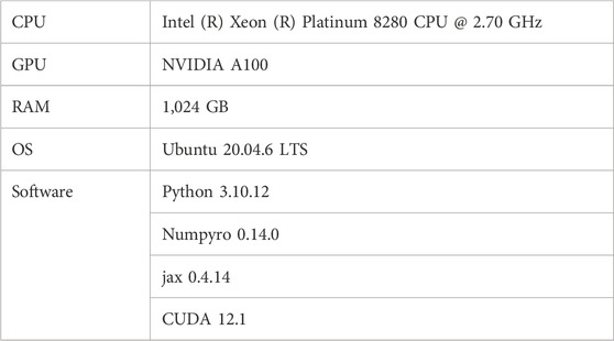
Table 1. Computational environment used for validation.

3.2 Creation of simulation data for validation

Based on the nucleic acid drug Fomivirsen (Perry and Balfour, 1999) (ID: A), two impurities with modified base sequences were added, and MS spectra for a total of three constituents were generated using simulation methods presented in the prior research (Tomono et al., 2024). Specific details were provided in Table 2. This setup replicated a system where the principal constituent’s isotopic distribution was mixed with the spectra of the impurities. The mutation from C (Cytosine) to U (Uracil), known as deamination, can occur during the synthesis process due to solvent conditions and thermal stress (Gao, Choudhry, and Cao, 2018; Stavnezer, 2011).

Table 2

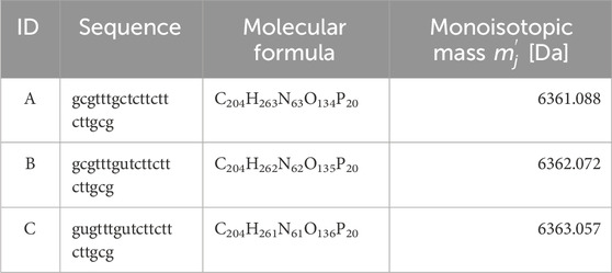
Table 2. Settings for constituent spectrum generation.

The single constituents A to C were combined according to the 10 combinations listed in Table 3. These combinations included both three-constituents mixtures (A, B, and C) and two-constituents mixtures (A and B, A and C, or B and C). To verify the accuracy of ion count inference, the ion counts of constituents A, B, and C were mixed at a ratio of 200,000:200,000 and 200,000:20,000. The reason for testing both balanced and imbalanced mixing ratios was to validate if our proposed algorithm tends to provide appropriate ratios of multiple constituents whether their actual ratios were balanced or imbalanced. When the ratio of ion counts between constituents was 10:1, the algorithm should not excessively provide less imbalanced ratios. This setup enabled the analysis of complex mixtures consisting of a few constituents. For instance, the standards for total desamido impurity and total impurities in injectable glucagon are set at 14% or less and 31% or less, respectively (Bao et al., 2022). To ensure rigor, we selected a stricter ratio of 10:1 (10%), which is below these standards yet sufficiently impactful to be considered as impurities. Additionally, the 10 patterns of combinations of each constituent were selected to comprehensively evaluate differences of 1 Da due to deamidation, while also considering workload required for our experimental performance evaluation and the constraints of a budget.

Table 3

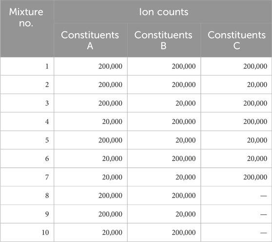
Table 3. Combinations of constituents when generating spectra.

We set the number of chargeable sites $l_j$ to 224 and the charge rate $v_j$ to 0.035. This was done to ensure that the generated spectra closely resembled real data. Then, we generated the test spectra listed in Table 3.

Next, we generated the MS/MS spectra of these mixture. The sequences, molecular formulas, monoisotopic masses, and conversion rates of the fragments generated from the dissociation of constituents A, B, and C are defined in Table 4. The MS/MS spectra were generated using these parameters. This time, we selected five peaks in ascending order of $m/z$ from the most prominent isotopic distribution, and we assumed two fragment constituents. Thus, $d_{\mathit{max}}$ was 5, and $f_{\mathit{max}}$ was 2.

Table 4

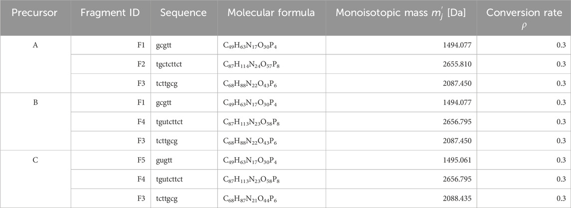
Table 4. Settings for constituent spectrum generation.

3.3 Evaluation of accuracy in inferred constituent counts

We estimated the optimal parameters for assumed constituent count models. Table 5 presents the logarithm of the maximum posterior probabilities of each model. By selecting the constituent count that maximizes the logarithm of the posterior probability in each mixture, we inferred the number of constituents present in each mixture. Our method successfully inferred the true number of constituents in 80% of cases (8 out of 10 datasets). In the two cases where estimation failed, it is possible that the algorithm converged to a different local minimum.

Table 5

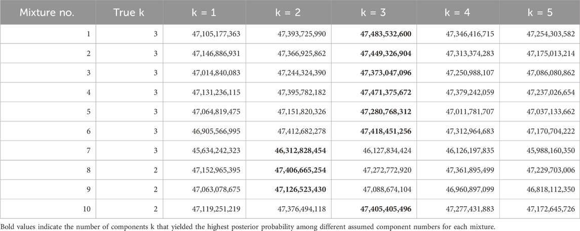
Table 5. Logarithmic the maximum posterior probability assuming each constituent count.

Currently, there are no established guidelines for the quality control of nucleic acid-based pharmaceuticals (International Council for Harmonisation, 2023; World Health Organization, 2018). Therefore, we believe this result serves as a valuable benchmark for identifying the presence and quantity of impurities in pharmaceuticals and implementing appropriate corrective measures. However, there is still room for improvement in its accuracy.

3.4 Accuracy of parameter inference

Table 6 shows the optimal monoisotopic mass of the models of the selected number of constituents for each mixture, as described in Table 3. The median error was −0.005 Da, the average error in monoisotopic mass was −0.282 Da, and the maximum error was −1.840 Da. The standard deviation was 0.552 Da. The distribution of these errors is shown in Figure 1. As observed in the box plot in Figure 1, the errors in the monoisotopic masses inferred by the proposed method are discretely distributed approximately 1 Da apart, corresponding to the mass differences between isotopes. The extreme case of No. 6, which produced the maximum error of −1.840 Da, can also be explained by this discrete distribution. This large error is likely caused by the posterior probabilities of the monoisotopic masses being distributed in a comb-like pattern (Tomono et al., 2024), increasing the chances of the algorithm converging to a local minimum 1–2 steps away. However, no clear trend was observed between the ion count ratios of the constituents and the error magnitudes. Using the mean as the representative value and all data from No. 1 to No. 10, the 95% confidence interval calculated using the t-distribution (Student, 1908) ranges from −0.721 Da to +0.157 Da. This indicates the method could potentially be used to investigate the causes of impurities that occur with a difference of 1 Da (Rentel et al., 2019; Pourshahian, 2021).

Table 6

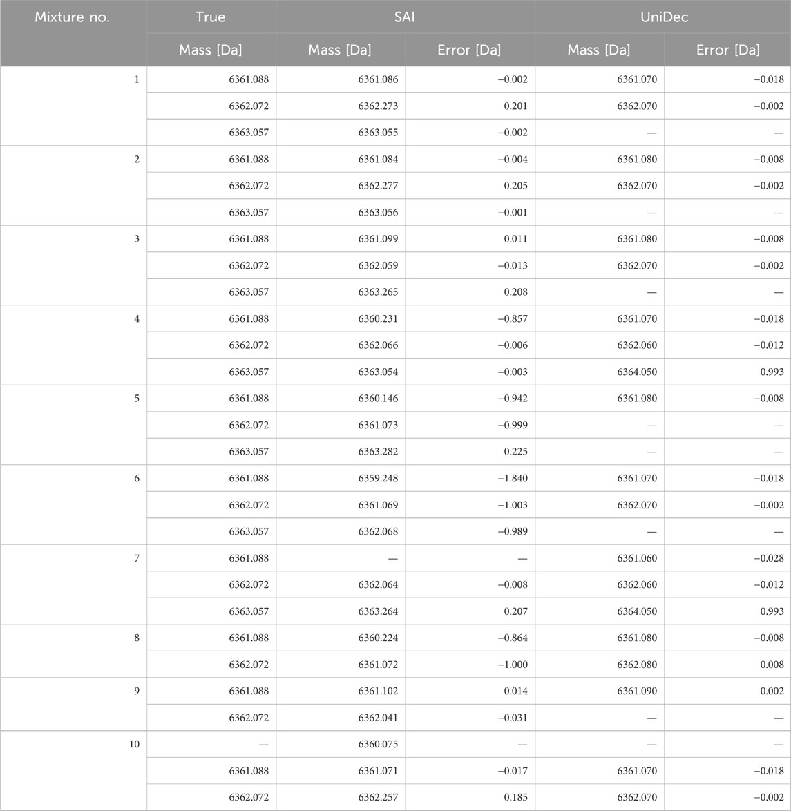
Table 6. Optimal monoisotopic masses of the model with the maximum posterior probability.

Figure 1

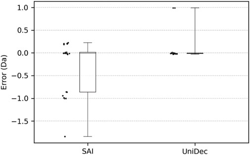
Figure 1. Distribution of errors in the inferred monoisotopic masses (excluding points that the algorithm could not infer).

Additionally, the inferred ion counts for each constituent showed errors with a median of 1.1 times the true values, averaging up to twice the true values, with some errors reaching up to twelve times the true values, as shown in Table 7. This was thought to be due to the trade-off relationship between the ion counts of different constituents; that was, a decrease in the ion count of one constituent was compensated by an increase in another. This was further supported by the fact that the average error across the total ion counts of all constituents stabilized at 8% of the true value. For instance, the standard for total desamido impurities and total impurities in injectable glucagon were, respectively, below 14% and 31%. Therefore, the accuracy of ion count inference in our proposed method was insufficient to assess the impact of impurities.

Table 7

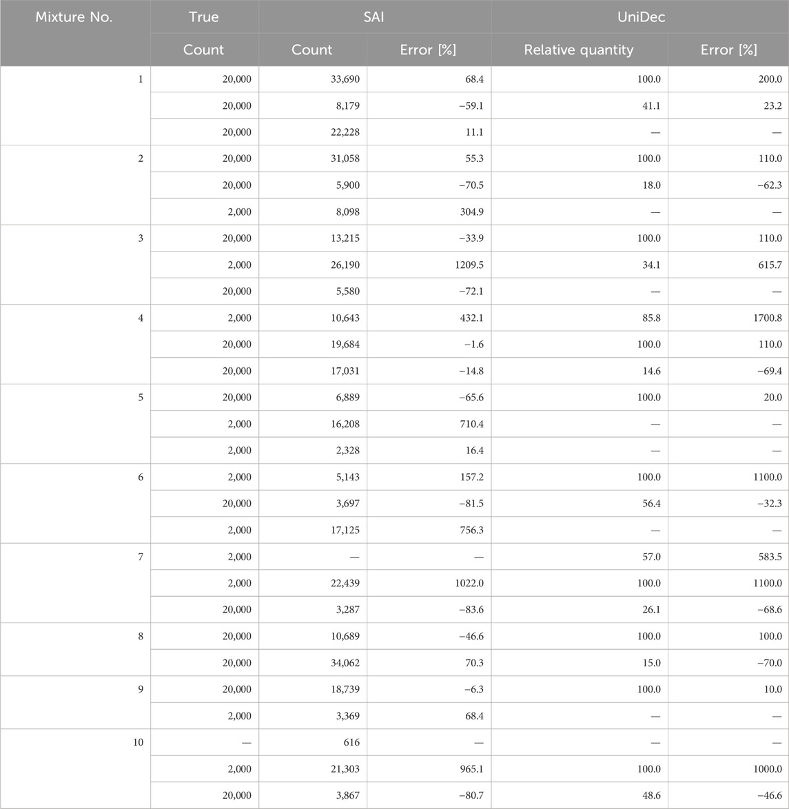
Table 7. Optimal ion counts and relative quantities of the model with the maximum posterior probability.

We also performed deconvolution on the same mixture data using UniDec, a popular deconvolution software, and compared the inference results. For this verification, we used UniDec (Version 7.0.1). The specific parameter settings used during this verification are shown in Table 8. The Mass Range was set to the same range as the proposed method, and Sample Mass Every (Da) was set to 0.1 to ensure sufficient detection of impurities with a difference of 1 Da. Default values were used for parameters not mentioned.

Table 8

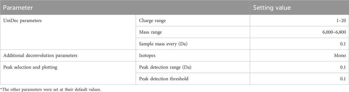
Table 8. UniDec setting parameters.

The accuracy of estimating the number of constituents was 40% (4 out of 10). This was thought to be because the UniDec algorithm, which iterated through multiple deconvolutions to arrive at the number of constituents, did not necessarily guarantee the accuracy of the constituent count. Note that using UniDec to determine the number of constituents was not its intended application. The median error of the monoisotopic mass inferred using UniDec was −0.008 Da, which is slightly worse than that of the proposed method. On the other hand, the average error was 0.091 Da, and the maximum error was 0.993 Da, both slightly better than those of the proposed method. However, in principle, accurate inference on the monoisotopic mass required precise identification of the number of constituents. The error in estimating the number of ions was, on average, 3.2 times the true value and up to 17 times at maximum. This result was not better than that of the proposed method.

For reference, Figure 2 presents a comparison between the spectrum of Mixture No. 1 and the spectrum reconstructed from its inferred parameters. Figure 2A provides an overview of the charge distribution, while Figure 2B offers a detailed view of the isotopic distribution. The gray vertical dashed lines in Figures 2A, B indicate the m/z of the fragmented ions. Additionally, Figures 2C, D display the MS/MS spectrum of the fragmented ion groups and its detailed view, respectively. The five graphs correspond to the five peaks in Figure 2B, each representing the MS/MS spectra of the ions contained in those peaks when they are fragmented. These results demonstrated that the generated spectrum closely matched with the observed data. Furthermore, the appearance of the MS/MS spectra was consistent with findings from prior research cited in references (Agthoven et al., 2019; Szalwinski et al., 2020; Gonzalez et al., 2022).

Figure 2

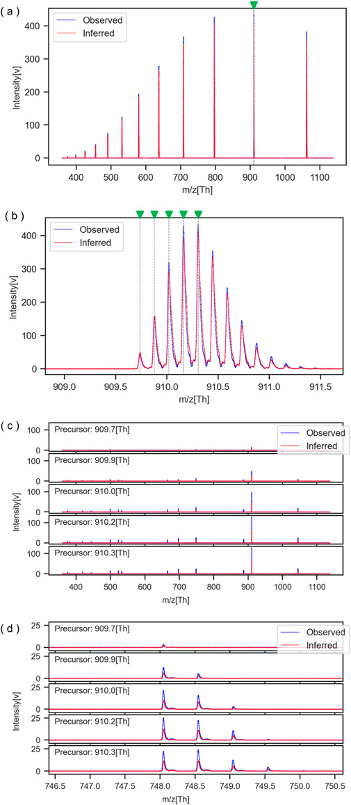
Figure 2. Comparison of observed and inferred spectra for Mixture No. 1. (A) MS spectrum overall view, (B) MS spectrum enlarged view, (C) MS/MS spectrum overall view, (D) MS/MS spectrum enlarged view.

4 Discussion

We confirmed that our proposed method allowed for accurate inference of parameters such as monoisotopic mass from simulated MS and MS/MS data of the nucleic acid drug Fomivirsen and its impurities, and it also successfully selected the correct number of constituents with an 80% probability, even in mixtures with a mass ratio of 10:1. These results were better compared to the 40% accuracy rate achieved with UniDec. This success was attributed to our approach of creating models for each constituent count, enabling comparative evaluation and selection of models for each constituent count. This capability suggests the presence of impurities in pharmaceuticals and could aid in the search for better synthesis conditions for medium to high molecular weight drugs, as well as in quality assurance in manufacturing facilities.

As shown in Table 6, we were able to infer monoisotopic mass with greater accuracy than previous studies (Tomono et al., 2024), with an average inference error of −0.282 Da, which was an improvement over the 1.348 Da error reported in prior research. Although this accuracy was slightly inferior to UniDec’s 0.091 Da, it was sufficient for distinguishing differences as small as 1 Da due to deamidation. We believe this improvement is due to the incorporation of the MS/MS spectra into the physical model, which increased the constraints on the model’s degrees of freedom. Additionally, the use of the correlation-based likelihood contributed to more stringent constraints on the spectral shape.

As indicated in Table 7, the inferred ion quantities for each constituent showed an average relative error of twice the true value. Although a direct comparison with the prior studies, which used a 1:1 mixing ratio, was not straightforward due to our use of a 10:1 ratio, the results were favorable compared to UniDec, which had an average error of 3.2 times the true value. The errors observed in our proposed method might result from a trade-off among the ion quantities of each constituent, where a decrease in one was offset by an increase in another. Despite our expectations that incorporating MS/MS spectra would tighten inference constraints and enhance both mass and ion quantity accuracy, the performance fell short of expectations, failing to reduce the relative error to below the 10% threshold required for impurity analysis in nucleic acid drugs. A possible solution to these issues would be to represent the ion quantities as probability distributions. By accounting for the uncertainty in the ion quantities of constituents in the sample, an improvement in inference accuracy was expected.

Despite the sixfold increase in data volume due to the incorporation of MS/MS spectra as observational data, the analysis time per data point was 13 h. While this duration did not match the few seconds required by UniDec, it was less than half the time required by existing methods (Tomono et al., 2024) that use MCMC.

5 Conclusion

In this study, we assumed the numbers of constituents in a given sample and created models of MS and MS/MS mass spectrometry based on parameters such as monoisotopic mass and ion quantity. We then applied our proposed method, Spectral Annealing Inference (SAI), which effectively seeks the maximum posterior probability by optimizing parameters for the observed data. After obtaining the maximum posterior probability for each constituent count model, we selected the model that had the highest maximum posterior probability across all models. As a result, we successfully estimated the number of constituents and simultaneously inferred the monoisotopic mass with high accuracy.

Future challenges include adapting to complex samples with a large number of constituents and improving the accuracy of ion counts inference.

Data availability statement

The raw data supporting the conclusions of this article will be made available by the authors, without undue reservation.

Author contributions

TT: Conceptualization, Investigation, Methodology, Project administration, Software, Validation, Visualization, Writing–original draft. SH: Conceptualization, Writing–review and editing. JI: Writing–review and editing. TW: Conceptualization, Supervision, Writing–review and editing.

Funding

The author(s) declare that no financial support was received for the research, authorship, and/or publication of this article.

Acknowledgments

We extend our deepest gratitude to Yoshihiro Ueno³, Yusuke Tagawa³, and Daisuke Hiramaru^2,5 for their invaluable advice and coordination throughout the entire project. This manuscript was partially translated with the assistance of ChatGPT (GPT-4, OpenAI) as of September 2024. The final translation were reviewed and confirmed by the authors.

Conflict of interest

Authors TT and JI were employed by Shimadzu Corporation.

The remaining authors declare that the research was conducted in the absence of any commercial or financial relationships that could be construed as a potential conflict of interest.

Publisher’s note

All claims expressed in this article are solely those of the authors and do not necessarily represent those of their affiliated organizations, or those of the publisher, the editors and the reviewers. Any product that may be evaluated in this article, or claim that may be made by its manufacturer, is not guaranteed or endorsed by the publisher.

References

Agthoven, M. A. van, Lam, Y. P. Y., O’Connor, P. B., Rolando, C., and Delsuc, M.-A. (2019). Two-dimensional mass spectrometry: new perspectives for tandem mass spectrometry. Eur. Biophysics J. EBJ 48 (3), 213–229. doi:10.1007/s00249-019-01348-5

CrossRef Full Text | Google Scholar

Bao, Z., Cheng, Y.-C., Luo, M. Z., and Zhang, J. Y. (2022). Comparison of the purity and impurity of glucagon-for-injection products under various stability conditions. Sci. Pharm. 90 (2), 32. doi:10.3390/scipharm90020032

CrossRef Full Text | Google Scholar

Dasari, S., Wilmarth, P. A., Reddy, A. P., Robertson, L. J. G., Nagalla, S. R., and Larry, L. D. (2009). Quantification of isotopically overlapping deamidated and 18O-labeled peptides using isotopic envelope mixture modeling. J. Proteome Res. 8 (3), 1263–1270. doi:10.1021/pr801054w

PubMed Abstract | CrossRef Full Text | Google Scholar

Ferrige, A., Ray, S., Alecio, R., Ye, S., and Waddell, K. (2003). Electrospray-MS charge deconvolutions without compromise – an enhanced data reconstruction algorithm utilising variable peak modelling. Santa Fe, NM: American Society for Mass Spectrometry. Available at: https://positiveprobability.com/POSTERS/ASMS%202003.pdf.

Google Scholar

Ferrige, A. G., Seddon, M. J., Green, B. N., Jarvis, S. A., Skilling, J., and Staunton, J. (1992). Disentangling electrospray spectra with maximum entropy. Rapid Commun. Mass Spectrom. RCM 6 (11), 707–711. doi:10.1002/rcm.1290061115

CrossRef Full Text | Google Scholar

Gao, J., Choudhry, H., and Cao, W. (2018). Apolipoprotein B MRNA editing enzyme catalytic polypeptide-like family genes activation and regulation during tumorigenesis. Cancer Sci. 109 (8), 2375–2382. doi:10.1111/cas.13658

PubMed Abstract | CrossRef Full Text | Google Scholar

Gonzalez, L. E., Szalwinski, L. J., Sams, T. C., Dziekonski, E. T., and Cooks, R. G. (2022). Metabolomic and lipidomic profiling of Bacillus using two-dimensional tandem mass spectrometry. Anal. Chem. 94 (48), 16838–16846. doi:10.1021/acs.analchem.2c03961

PubMed Abstract | CrossRef Full Text | Google Scholar

International Council for Harmonisation (ICH) (2023). ICH Q2(R2): validation of analytical procedures. Geneva, Switzerland: International Council for Harmonisation.

Google Scholar

Kingma, D. P., and Jimmy, Ba. (2014). Adam: a method for stochastic optimization. ArXiv [Cs.LG]. doi:10.48550/arXiv.1412.6980

CrossRef Full Text | Google Scholar

Kingma, D. P., and Welling, M. (2013). Auto-encoding variational Bayes. ArXiv [Stat.ML]. Available at: http://arxiv.org/abs/1312.6114v11.

Google Scholar

Lucy, L. B. (1974). An iterative technique for the rectification of observed distributions. Astronomical J. 79 (June), 745. doi:10.1086/111605

CrossRef Full Text | Google Scholar

Mardia, K. V., and Jupp, P. E. (2008). Directional statistics. Limited, John: Wiley and Sons.

Google Scholar

Marty, M. T. (2020). A universal score for deconvolution of intact protein and native electrospray mass spectra. Anal. Chem. 92 (6), 4395–4401. doi:10.1021/acs.analchem.9b05272

PubMed Abstract | CrossRef Full Text | Google Scholar

Marty, M. T., Baldwin, A. J., Marklund, E. G., Hochberg, G. K. A., Benesch, J. L. P., and Robinson, C. V. (2015). Bayesian deconvolution of mass and ion mobility spectra: from binary interactions to polydisperse ensembles. Anal. Chem. 87 (8), 4370–4376. doi:10.1021/acs.analchem.5b00140

PubMed Abstract | CrossRef Full Text | Google Scholar

Neath, A. A., and Cavanaugh, J. E. (2012). The bayesian information criterion: background, derivation, and applications. WIREs Comput. Stat. 4 (2), 199–203. doi:10.1002/wics.199

CrossRef Full Text | Google Scholar

Pecori, R., Di Giorgio, S., Paulo Lorenzo, J., and Nina Papavasiliou, F. (2022). Functions and consequences of AID/APOBEC-Mediated DNA and RNA deamination. Nat. Rev. Genet. 23 (8), 505–518. doi:10.1038/s41576-022-00459-8

PubMed Abstract | CrossRef Full Text | Google Scholar

Perry, C. M., and Balfour, J. A. (1999). Fomivirsen. Drugs 57 (3), 375–380. doi:10.2165/00003495-199957030-00010

PubMed Abstract | CrossRef Full Text | Google Scholar

Pourshahian, S. (2021). Therapeutic oligonucleotides, impurities, degradants, and their characterization by mass spectrometry. Mass Spectrom. Rev. 40 (2), 75–109. doi:10.1002/mas.21615

PubMed Abstract | CrossRef Full Text | Google Scholar

Ranganath, R., Gerrish, S., and Blei, D. (2014). “Black box variational inference,” in Proceedings of the seventeenth international conference on artificial intelligence and statistics. Proceedings of machine learning research. Editors S. Kaski, and J. Corander (Reykjavik, Iceland: PMLR), 33, 814–822.

Google Scholar

Rentel, C., DaCosta, J., Roussis, S., Chan, J., Capaldi, D., and Bao, M. (2019). Determination of oligonucleotide deamination by high resolution mass spectrometry. J. Pharm. Biomed. Analysis 173 (September), 56–61. doi:10.1016/j.jpba.2019.05.012

PubMed Abstract | CrossRef Full Text | Google Scholar

Richardson, W. H. (1972). Bayesian-based iterative method of image restoration. J. Opt. Soc. Am. 62 (1), 55. doi:10.1364/josa.62.000055

CrossRef Full Text | Google Scholar

Sanghvi, Y. S. (2011). “A status update of modified oligonucleotides for chemotherapeutics applications,” in Current protocols in nucleic acid chemistry. Editor S. L. Beaucage, 1–22.

Google Scholar

Schwarz, G. (1978). Estimating the dimension of a model. Ann. Statistics 6 (2), 461–464. doi:10.1214/aos/1176344136

CrossRef Full Text | Google Scholar

Stavnezer, J. (2011). Complex regulation and function of activation-induced cytidine deaminase. Trends Immunol. 32 (5), 194–201. doi:10.1016/j.it.2011.03.003

PubMed Abstract | CrossRef Full Text | Google Scholar

Student (1908). The probable error of a mean. Biometrika 6 (1), 1. doi:10.2307/2331554

CrossRef Full Text | Google Scholar

Szalwinski, L. J., Holden, D. T., Morato, N. M., and Cooks, R. G. (2020). 2D MS/MS spectra recorded in the time domain using repetitive frequency sweeps in linear Quadrupole ion traps. Anal. Chem. 92 (14), 10016–10023. doi:10.1021/acs.analchem.0c01719

PubMed Abstract | CrossRef Full Text | Google Scholar

Tamara, S., den Boer, M. A., and Heck, A. J. R. (2022). High-resolution native mass spectrometry. Chem. Rev. 122 (8), 7269–7326. doi:10.1021/acs.chemrev.1c00212

PubMed Abstract | CrossRef Full Text | Google Scholar

Tomono, T., Hara, S., Nakai, Y., Takahara, K., Iida, J., and Washio, T. (2024). A bayesian approach for constituent estimation in nucleic acid mixture models. Front. Anal. Sci. 3. doi:10.3389/frans.2023.1301602

CrossRef Full Text | Google Scholar

Tranter, R. L. (2000). Design and analysis in chemical research. John Wiley and Sons.

Google Scholar

Weinberg, W. C., Frazier-Jessen, M. R., Wu, W. J., Weir, A., Hartsough, M., Keegan, P., et al. (2005). Development and regulation of monoclonal antibody products: challenges and opportunities. Cancer Metastasis Rev. 24 (4), 569–584. doi:10.1007/s10555-005-6196-y

PubMed Abstract | CrossRef Full Text | Google Scholar

Wingate, D., and Weber, T. (2013). Automated variational inference in probabilistic programming. ArXiv E-Prints, January, arXiv:1301.1299.

Google Scholar

World Health Organization (WHO) (2018). Good practices for pharmaceutical quality control laboratories. Geneva, Switzerland: World Health Organization.

Google Scholar

Zhang, J., Gonzalez, E., Hestilow, T., Haskins, W., and Huang, Y. (2009). Review of peak detection algorithms in liquid-chromatography-mass spectrometry. Curr. Genomics 10 (6), 388–401. doi:10.2174/138920209789177638

PubMed Abstract | CrossRef Full Text | Google Scholar

Zhang, K., and Alecio, R. (1998). “A novel approach to the automated analysis of peptide mapping data,” in Proceedings of the Estonian academy of Sciences. Biology, ecology = eesti teaduste akadeemia toimetised. Okoloogia: Bioloogia.

Google Scholar