 Frank Westad1,2*
 Geir Rune Flåten3
- 1Department of Engineering Cybernetics, Norwegian University of Science and Technology, Trondheim, Norway
- 2Idletechs AS, Trondheim, Norway
- 3AspenTech Norway AS, Lysaker, Norway
This perspective article reviews how the chemometrics community approached non-linear methods in the early years. In addition to the basic chemometric methods, some methods that fall under the term “machine learning” are also mentioned. Thereafter, types of non-linearity are briefly presented, followed by discussions on important aspects of modeling related to non-linear data. Lastly, a simulated data set with non-linear properties is analyzed for quantitative prediction and batch monitoring. The conclusion is that the latent variable methods to a large extent handle non-linearities by adding more linear combinations of the original variables. Nevertheless, with strong non-linearities between the X and Y space, non-linear methods such as Support Vector Machines might improve prediction performance at the cost of interpretability into both the sample and variable space. Applying multiple local models can improve performance compared to a single global model, of both linear and non-linear nature. When non-linear methods are applied, the need for conservative model validation is even more important. Another approach is pre-processing of the data which can make the data more linear before the actual modeling and prediction phase.
1 Introduction
Based on personal experience from teaching multivariate analysis in academia and for various industry verticals it seems to be a notion in some scientific communities that basic chemometric methods such as PCA and PLSR cannot handle non-linearities. This is to some extent correct although, e.g., a banana-shaped data structure can be modeled by three subsequent linear components, so it is not necessarily so that a piece-wise spline function is needed for achieving a model with the required accuracy and precision. Within spectroscopy, many published papers apply PLS regression on spectra for multivariate calibration Martens and Næs (1984) in reflectance units. Although there exists a logarithmic relation between reflectance and concentration, these models generally show no significant difference in precision performance compared to models in absorbance units. However, for the interpretation of raw data and concentration of the analytes, the absorbance unit is preferred.
Already in the early days of what falls under what is named chemometrics, various approaches for the frequently applied methods for handling non-linearities were developed and investigated. For the basic multivariate method Principal Component Analysis (PCA) Jackson (2005), kernel-PCA Schölkopf et al. (1998) and PCA combined with neural networks Gallo and Capozzi (2019) are among the methods that have been evaluated. Independent Component Analysis (ICA) is another method for analyzing one data table that also has its non-linear equivalents Hyvarinen et al. (2019). In the case of regression for quantitative prediction, the basic work-horse has been Partial Least Squares Regression (PLSR) Gerlach et al. (1979). Non-linear variants of PLSR include polynomial Durand (2001) and spline PLSR Wold (1992), where the so-called inner relation between the X and Y space, or more precisely, between the covariance space of (X, Y) and Y, is modeled as a non-linear function. Another approach is to add non-linear features to the original variables or add interaction and squares of the score vectors Vogt (1989). Thus, non-linearity is handled without explicitly applying non-linear methods.
Artificial Neural Networks (ANN) relatively early caught the interest in the chemometric community Wythoff (1993). In more recent times, Support Vector Machines (SVM) Boser et al. (1992) and tree-based methods such as Random Forests (RF) Ho (1995) have gained popularity. Convolutional Neural Nets (CNN) Fukushima (1988), Krizhevsky et al. (2012) and autoencoders Rumelhart et al. (1986) are among the most applied methods for image classification. In the early 90’s with the computer power at that time there was no option to apply CNN with thousands of features and multiple layers for classification, therefore less computationally demanding methods were the viable options.
Various types of non-linearities may occur given the actual application:
• Non-linearities in X and/or Y
• Non-linearities between X and Y
• Change in the correlation structure throughout a batch process, giving non-linear behavior in the time series
• Non-stationary continuous time-series
2 Materials and methods
2.1 Data
2.1.1 Fermentation process
The selected data for this study is a simulated data set based on a biological first-principle model of a fermentation reaction Lei et al. (2001). The data has a total of ten process variables.
The data were divided into a training and test set, where two of the test set batches have known anomalies for given periods of time. The data were subject to two types of analysis: a) For modeling and monitoring batch processes, and b) For regression modeling.
The objective of including this data set for batch modeling is to present data that are non-linear along the time axis and with non-linearities occurring at different points of time for the individual variables. And, as usual for batch processes, the batches are not of the same lengths.
Line plots of the raw data for ethanol concentration and oxygen uptake rate are shown in Figure 1. As can be seen, the concentration at different points in time varies between the batches, and differently for the two variables shown. However, in the multivariate space, this does not pose a problem as such as can be seen in Section 3. For more details about the batch modeling method applied, see Section 2.2.1.
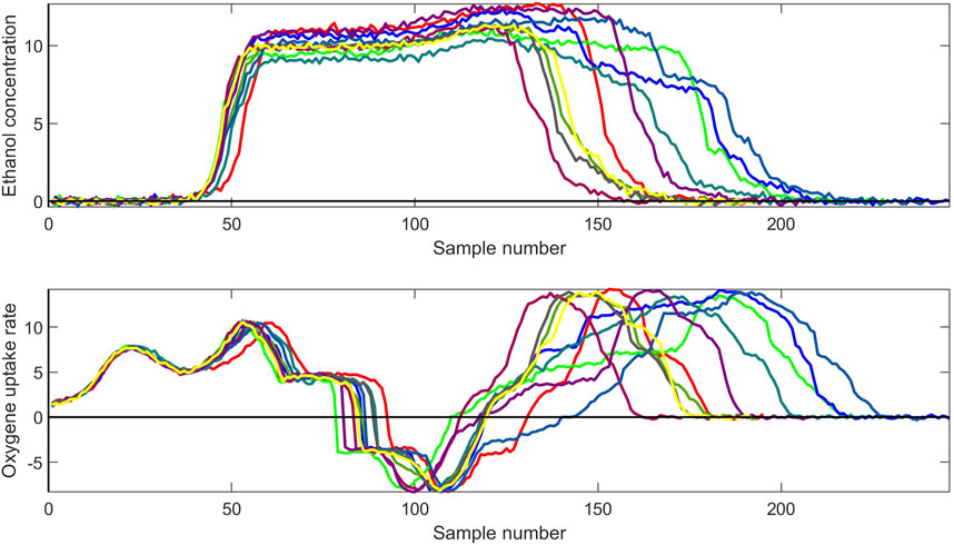
Figure 1. Raw data for two variables.
For case b) the focus is on prediction of the biomass from the nine other chemical variables, see Section 2.1.1.
2.2 Theory
2.2.1 Batch modeling
Batch modeling has been a topic of interest for decades Nomikos and MacGregor (1995). The most common approach is to unfold the three-dimensional data either batch-wise or time-wise and analyze the data with Principal Component Analysis, PCA.
As the batches in most real processes have different lengths, this needs to be handled both in the modeling and monitoring phases. Some approaches for handling this challenge without time warping can be found in (Westad et al., 2015; Rocha de Oliveira and de Juan, 2022). These two papers make use of the concept of relative time as opposed to clock time. In this case, the unfolding is performed such that the rows are all time points ordered sequentially for all batches whereas the columns are the variables. Two advantages of the relative time approach are that various batch lengths do not pose a problem, nor if some batches were acquired with various sampling frequencies. Even a case where batches have missing values for some time points is handled intrinsically; the trajectory will continue at the given relative time. Although some literature claims that time warping of the various batches is a necessary step in batch modeling, this is not correct. One can always warp batches to the same lengths with correlation-optimized warping or other methods, but this may distort the inherent time-dependent correlations between the variables. Furthermore, time warping of batches cannot easily be applied when monitoring new batches as the batch length is not known a priori.
2.2.2 Latent variable regression
There exist many regression methods that are based on latent variables. The difference between them lies in how the covariance between X and Y is modeled. One of the most used methods for prediction is Partial Least Squares Regression (PLSR) as it has been shown to give a good balance between fit and precision Høskuldsson (1996) by finding eigenvectors that maximize the covariance between X and Y. For PLS regression specifically, there exist many algorithms that are preferred subject to the dimensionality of the data; the number of samples, the number of x-variables, and the number of y-variables (de Jong, 1993; Lindgren et al., 1993; Dayal and Macgregor, 1997). Details about the many methods and algorithms are not explored in this paper as it is out of the scope, PLS regression is briefly described.
2.2.2.1 PLS regression
The general form of the PLS regression model is:
T is the matrix of scores, P are the X-loadings, Eq. 1 and Q are the Y-loadings, Eq. 2. E and F are the residual matrices after the optimal number of factors have been extracted.
PLSR maximizes the covariance between X and Y. The covariance for each factor a is expressed by the loading weights vector, Eq. 3:
That is, finding the first eigenvector of
The expression for the regression coefficients is given by, Eq. 4:
2.2.3 Local weighted regression
Locally weighted regression (LWR) copes with non-linear data structures by modeling a subset of the training data on-the-fly based on the distance to the new sample Cleveland and Devlin (1988). For latent variable methods, the new sample is projected onto the score space from a global model. LWR requires tuning of hyper-parameters, e.g., how many samples to include in the local models, alternatively a threshold for selecting samples within a certain distance, or the type of distance measure. The rank of the local models must be assessed unsupervised, which might be a challenge.
2.2.4 Support vector machine regression
Support Vector Machine Regression (SVMR or SVR) is the regression alternative to support vector machine classification (SVMC) Smola and Schölkopf (2004). The two methods both make use of various kernels to handle non-linearities. Where SVMC uses support vectors to find the best subset of samples to find the optimal decision boundaries, SVR defines an error margin epsilon, ϵ, to tolerate small errors, thereby weighting the larger errors in the modeling phase. Another parameter that needs to be tuned for non-linear kernels is γ. It governs for which distance to the boundary samples should be considered; a small gamma means samples far away and a large gamma will focus on the smaller distances.
3 Discussion
This section first discusses vital aspects of modeling with a focus on non-linear behavior before reporting results from batch monitoring and prediction applications.
Some vital aspects regarding multivariate modeling/machine learning are:
• Computational complexity
• Interpretability
• Model validation and robustness
• Outlier detection
3.1 Computational complexity and need for many samples
As mentioned above, compared to the early days of chemometrics, one can with today’s computers easily try and reject 1000s of models in search of the “best” one. As the basic methods PCA and PLSR do not need extensive hyper-parameter tuning; the hyper-parameter is the number of latent variables, there is not necessarily a need for a huge number of samples for training the models. Another aspect is that for building quantitative models, providing representative training samples within chemistry and biology required considerable manual work. Many real-life applications make use of multichannel instruments such as NIR spectroscopy for in-line, on-line, or at-line prediction of constituents of interest. Therefore, most data sets for multivariate calibration had more variables than samples which either required variable selection to apply Multiple Linear Regression (MLR) or latent variable methods such as PLSR. A rule of thumb is to have as many samples as six times the number of latent variables for training (calibration). The test set should analogously be of sufficient size.
As the number of samples increases, the use of non-linear methods which rely on tuning of hyperparameters becomes more relevant. SVR is an alternative also with a moderate number of samples as the number of hyperparameters to tune is limited. The optimal settings are found by use of a grid search and applying proper validation. Comparison of prediction performance for PLSR and non-linear methods has been the topic in numerous papers, e.g., for many applications within chemistry, food, and feed, e.g., Luinge et al. (1995),Liu et al. (2019). Whether ANN outperforms PLSR is dependent on the nature of the data. ANN requires in general more samples than PLSR and the effort to acquire reference data (Y) for quantitative models is often time and/or labor-intensive. A comparison of ANN and various regression methods for medical applications is given in Sargent (2001). Another comparison is given in Dreiseitl and Ohno-Machado (2002) where it is highlighted that there might be a publication bias for such comparisons. For classification purposes, it might be less demanding although labeling might still be a semi-manual task, e.g., for image classification applications. Also, there is a tendency to compare results from the basic PLSR with the ANN results following an extensive search for the best hyperparameters. A statistical test is rarely performed to evaluate if the results are significantly different although the numerical results may indicate so. Additionally, one should always take into account the precision of the reference method when comparing estimated prediction errors.
The combination of latent variables and ANN may be seen as the “the best of both worlds.” Firstly, error in the X-matrix is removed before the ANN, secondly, with a reduced number of input variables as the orthogonal score vectors are used as inputs, the optimization of hyperparameters is numerically less extensive Gemperline et al. (1991). Furthermore, it enables outlier detection, see Section 3.4.
3.2 Interpretability
Another reason why the basic methods are still in use in real-time in the industry in the era of AI/ML is the aspect of interpretability. Chemometrics has favored methods that can be interpreted both in the sample and variable domains. Numerous tutorials and textbooks on the topic of interpretation in latent multivariate methods have been published, e.g., Bro and Smilde (2014) and Esbensen et al. (2018). There are also application-specific approaches given the nature of the data, e.g., for chromatography/hyphenated systems, spectroscopy, food and agriculture and process data. Chemometrics has also had a tradition of extracting pure signals from complex systems for confirmation of theory and understanding causality de Juan and Tauler (2021),Johnsen et al. (2017). Some non-linear methods provide ranking of variable importance, such as SVM and Random Forests, but few methods offer a look into both domains, which is essential for model interpretation giving the underlying domain-specific knowledge and type of process.
Visualization of meta-information in score plots has often revealed product and process quality issues that are not found in the numerical data themselves. A typical example of this is how to convey differences in quality due to non-controllable sources of variance, e.g., raw materials, season, and sensor differences. For an example of a score plot, see Figure 2 in Section 3.5. This is closely connected to proper validation, see Section 3.3.
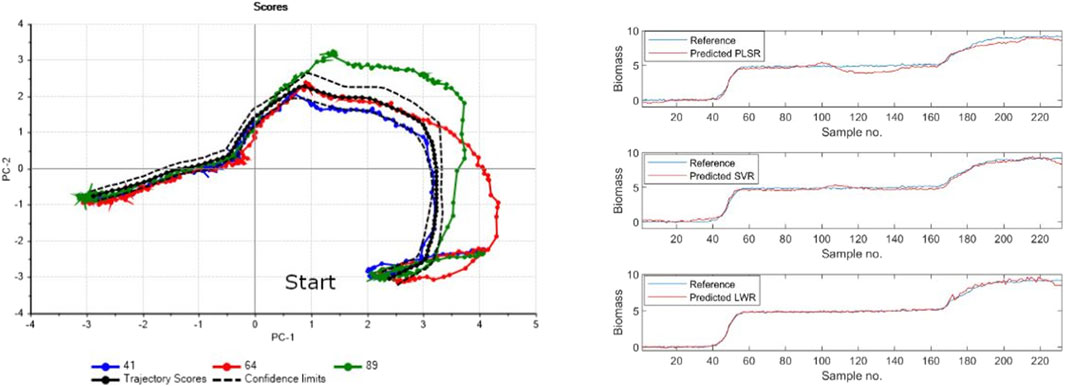
Figure 2. Projection of new batches onto the model (left), and predicted and reference values for biomass (right).
3.3 Model validation
Related to modeling with non-linear methods, the bias-variance trade-off is an important aspect. As the models become more complex, the bias will decrease at the cost of higher variance, i.e., decreased model stability. Models with high bias suffer from underfitting; not capturing the systematic variance in the model, vs. overfitting; noise is modeled as relevant variance. Setting up the proper validation scheme(s) is of great importance for deciding on the model complexity. For all real processes, there is one or more reasons to group the samples according to underlying categorical information. Randomly dividing the data into training and test sets 1000 times will in most cases give too optimistic models. This is the case although an independent test set is defined Westad and Marini (2015).
Furthermore, for methods with the need for extensive hyper-parameter tuning, one needs a third set of samples as the second set is used to fine-tune the model parameters; this is the case for methods that cannot be cross-validated because the model structure is not the same between cross-validation segments. This also makes it difficult to estimate uncertainty in the model parameters, e.g., for variable selection. This was not recognized in the early days of ANN, as one was erroneously selecting the best model based on the performance of the second set, and it still seems to be a challenge in some communities Kapoor and Narayanan (2023). As the terminology varies in different communities, there is no consensus on how to label sets two and three; the first set is named “training” set in the machine learning community, and “calibration” set within chemometrics. And even if a complex model performs well on a test set, there is no guarantee that the model is robust toward prediction of unseen data Ball (2023), Naddaf (2024).
3.4 Outlier detection
Another important aspect of modeling is outlier detection. One thing is to handle outliers in the modeling phase, for which there are many methods and approaches. However, one may argue that outlier detection is even more important in the prediction phase. As is known, with the latent variable methods one can distinguish between two types of outliers; within the model space and in the residual space Jackson (2005). Drilling down into variable contributions and individual sample residuals allows for root cause analysis and knowledge-generating modeling and prediction Westerhuis et al. (2000).
3.5 Batch modeling and monitoring of the fermentation data
A batch model based on ten batches was developed by estimating a trajectory and critical limits as described in Westad et al. (2015). The model was cross-validated by repeatedly taking out one batch and modeling the remaining ones as this is the proper validation scheme in a real-life situation. This will influence how the dynamic confidence intervals are estimated. Three new batches were projected onto this model, of which two had been deliberately altered to illustrate outlying batches. The projected results are shown on the left of Figure 2, with a 95% confidence interval around the estimated trajectory. Interestingly enough, the two batches that were simulated to be outliers show deviations only for parts of the trajectory. Furthermore, as the model space defined by the principal components represents the system in relative time, the number of samples does not influence the projection. If some samples had been taken out for the new batches, it would not pose any problem.
3.6 Prediction of the response variable biomass
For this example, two batches were selected for establishing a model, with a total of 432 samples. The independent variables were the first nine analytes in the data set, whereas biomass was defined as the dependent variable. One batch was selected as a test set, a total of 243 samples. The global PLSR model had an optimal dimensionality of 7 as assessed by cross-validation. A grid search with ten segment cross-validation was performed for a polynomial SVR model, giving a gamma of 10 and an ϵ of 0.1. LWR was run with 40 local samples. The unsupervised assessment of the optimal number of factors for the individual models was found from the cross-validated RMSE with a threshold of 0.02, i.e., if including a new factor did not reduce RMSECV with at least 2% from the previous factor, this factor was not added to the model. The prediction errors (RMSEP) for the test set for PLSR, SVR, and LWR were 0.45, 0.27, and 0.18 respectively. Bartlett’s test on the residuals revealed that there are significant differences between all three models. Although the numerical values are small, the percent-wise differences are relatively large. The global PLSR model had a correlation of 0.991 for the test set, the RMSE after centered and scaled data for the test set was 2.811.
3.7 Future directions
As shown in this overview, there are several established approaches to handling the different types of non-linearities. Their strengths include interpretability and low computational cost. The case study also demonstrates how the established methods can be used for complex non-linearity problems like varying non-linearity over time, keeping interpretability, and low computational costs. There are few examples where the traditional methods with adaptations are falling short although strong non-linearities and huge data sets do create some challenges and occasionally problems that the traditional methods cannot solve Raccuglia et al. (2016), Stokes et al. (2020), Senior et al. (2020). Baum gives an overview of recent trends in analytical chemistry and AI, Baum et al. (2021).
The ever-growing computational capability has rightfully created a lot of excitement in the analytics world. Particularly as the parallel improvements in sensors and systems are generating bigger and bigger data sets. Thus, computational methods like neural networks, for instance, are reinvigorated and currently both relevant and attainable. The challenge is to not get blinded by the brute force opportunity and ensure that well-founded practices for model building, validation, and usage are retained. The problem of wrongful use of powerful data analytical methods was noticed even for the traditional methods Kjeldahl and Bro (2010), and the problem is magnified with the increasing power of modern methods within ML/AI Ioele et al. (2011). The growing complexity of the models introduces the additional challenge of transparency where it is unclear how the result was generated—which features were used, how was the concentration estimated, etc. On the other hand, the more complex methods do carry a promise of the ability to solve more complex problems if used correctly.
The challenge of non-linearity in data is in some ways more attainable than ever although more advanced measurement methods might introduce new challenges. There is a library of traditional methods with an adaption that already solves most non-linear problems, and the attainability of more advanced data analytical methods provides a reserve of powerful approaches for non-linear problems currently not handled well. Our recommendation is to keep using the traditional methods for weak non-linear systems. The ML/AI approaches still have some challenges w.r.t. validation, interpretability, and reproducibility, and should in our opinion be reserved for problems that require more advanced tools to be solved.
Data availability statement
Publicly available datasets were analyzed in this study. This data can be found here: https://github.com/jogonmar/MVBatch/blob/master/examples/SACCHA_D.mat.
Author contributions
FW: Formal Analysis, Methodology, Writing–original draft, Writing–review and editing, Conceptualization. GF: Formal Analysis, Methodology, Writing–original draft, Writing–review and editing, Conceptualization.
Funding
The author(s) declare that no financial support was received for the research, authorship, and/or publication of this article.
Conflict of interest
Author FW was employed by Idletechs AS. Author GF was employed by AspenTech Norway AS.
The author(s) declared that they were an editorial board member of Frontiers, at the time of submission. This had no impact on the peer review process and the final decision.
Publisher’s note
All claims expressed in this article are solely those of the authors and do not necessarily represent those of their affiliated organizations, or those of the publisher, the editors and the reviewers. Any product that may be evaluated in this article, or claim that may be made by its manufacturer, is not guaranteed or endorsed by the publisher.
References
Ball, P. (2023). Is AI leading to a reproducibility crisis in science? Nature 624, 22–25. doi:10.1038/d41586-023-03817-6
Baum, Z. J., Yu, X., Ayala, P. Y., Zhao, Y., Watkins, S. P., and Zhou, Q. A. (2021). Artificial intelligence in chemistry: current trends and future directions. J. Chem. Inf. Model. 61, 3197–3212. doi:10.1021/acs.jcim.1c00619
Boser, B. E., Guyon, I. M., and Vapnik, V. N. (1992). “A training algorithm for optimal margin classifiers,” in Proceedings of the 5th annual workshop on computational learning theory (COLT’92). Editor D. Haussler (Pittsburgh, PA, USA: ACM Press), 144–152.
Bro, R., and Smilde, A. K. (2014). Principal component analysis. Anal. Methods 6, 2812–2831. doi:10.1039/C3AY41907J
Cleveland, W. S., and Devlin, S. J. (1988). Locally weighted regression: an approach to regression analysis by local fitting. J. Am. Stat. Assoc. 83, 596–610. doi:10.1080/01621459.1988.10478639
Dayal, B. S., and Macgregor, J. F. (1997). Improved pls algorithms. J. Chemom. 11, 73–85. doi:10.1002/(sici)1099-128x(199701)11:1<73::aid-cem435>3.0.co;2-#
de Jong, S. (1993). Simpls: an alternative approach to partial least squares regression. Chemom. Intelligent Laboratory Syst. 18, 251–263. doi:10.1016/0169-7439(93)85002-X
de Juan, A., and Tauler, R. (2021). Multivariate curve resolution: 50 years addressing the mixture analysis problem – a review. Anal. Chim. Acta 1145, 59–78. doi:10.1016/j.aca.2020.10.051
Dreiseitl, S., and Ohno-Machado, L. (2002). Logistic regression and artificial neural network classification models: a methodology review. J. Biomed. Inf. 35, 352–359. doi:10.1016/S1532-0464(03)00034-0
Durand, J.-F. (2001). Local polynomial additive regression through pls and splines: plss. Chemom. Intelligent Laboratory Syst. 58, 235–246. doi:10.1016/S0169-7439(01)00162-9
Esbensen, K., Swarbrick, B., Westad, F., Whitcomb, P., and Anderson, M. (2018). “Multivariate data analysis: an introduction to multivariate analysis,” in Process analytical technology and quality by design (CAMO).
Fukushima, K. (1988). Neocognitron: a hierarchical neural network capable of visual pattern recognition. Neural Netw. 1, 119–130. doi:10.1016/0893-6080(88)90014-7
Gallo, C., and Capozzi, V. (2019). Feature selection with non linear PCA: a neural network approach. J. Appl. Math. Phys. 7, 2537–2554. doi:10.4236/jamp.2019.710173
Gemperline, P., Long, J. R., and Gregoriou, V. G. (1991). Nonlinear multivariate calibration using principal components regression and artificial neural networks. Anal. Chem. 63, 2313–2323. doi:10.1021/ac00020a022
Gerlach, R. W., Kowalski, B. R., and Wold, H. O. (1979). Partial least-squares path modelling with latent variables. Anal. Chim. Acta 112, 417–421. doi:10.1016/S0003-2670(01)85039-X
Ho, T. K. (1995). “Random decision forests,” in Proceedings of 3rd international conference on document analysis and recognition (IEEE), 1, 278–282.
Høskuldsson, A. (1996) Prediction methods in science and technology, 1. Basic theory (Thor Publishing.
Hyvarinen, A., Sasaki, H., and Turner, R. (2019). “Nonlinear ica using auxiliary variables and generalized contrastive learning,” in The 22nd international conference on artificial intelligence and statistics (United States: Journal of Machine Learning Research), 859–868.
Ioele, G., De Luca, M., Dinç, E., Oliverio, F., and Ragno, G. (2011). Artificial neural network combined with principal component analysis for resolution of complex pharmaceutical formulations. Chem. Pharm. Bull. 59, 35–40. doi:10.1248/cpb.59.35
Johnsen, L. G., Skou, P. B., Khakimov, B., and Bro, R. (2017). Gas chromatography – mass spectrometry data processing made easy. J. Chromatogr. A 1503, 57–64. doi:10.1016/j.chroma.2017.04.052
Kapoor, S., and Narayanan, A. (2023). Leakage and the reproducibility crisis in machine-learning-based science. Patterns 4, 100804. doi:10.1016/j.patter.2023.100804
Kjeldahl, K., and Bro, R. (2010). Some common misunderstandings in chemometrics. J. Chemom. 24, 558–564. doi:10.1002/cem.1346
Krizhevsky, A., Sutskever, I., and Hinton, G. E. (2012). “Imagenet classification with deep convolutional neural networks,” in Advances in neural information processing systems. Editors F. Pereira, C. Burges, L. Bottou, and K. Weinberger (United States: Curran Associates, Inc.), 25.
Lei, F., Rotbøll, M., and Jørgensen, S. B. (2001). A biochemically structured model for saccharomyces cerevisiae. J. Biotechnol. 88, 205–221. doi:10.1016/S0168-1656(01)00269-3
Lindgren, F., Geladi, P., and Wold, S. (1993). The kernel algorithm for pls. J. Chemom. 7, 45–59. doi:10.1002/cem.1180070104
Liu, X., Liu, C., Shi, Z., and Chang, Q. (2019). Comparison of prediction power of three multivariate calibrations for estimation of leaf anthocyanin content with visible spectroscopy in prunus cerasifera. PeerJ 7, e7997. doi:10.7717/peerj.7997
Luinge, H., van der Maas, J., and Visser, T. (1995). Partial least squares regression as a multivariate tool for the interpretation of infrared spectra. Chemom. Intelligent Laboratory Syst. 28, 129–138. doi:10.1016/0169-7439(95)80045-B
Martens, H., and Næs, T. (1984) Multivariate calibration. Dordrecht: Springer Netherlands, 147–156. doi:10.1007/978-94-017-1026-8_5
Naddaf, M. (2024). Mind-reading devices are revealing the brain's secrets. Nature 626, 706–708. doi:10.1038/d41586-024-00481-2
Nomikos, P., and MacGregor, J. F. (1995). Multivariate spc charts for monitoring batch processes. Technometrics 37, 41–59. doi:10.1080/00401706.1995.10485888
Raccuglia, P., Elbert, K. C., Adler, P. D. F., Falk, C., Wenny, M. B., Mollo, A., et al. (2016). Machine-learning-assisted materials discovery using failed experiments. Nature 533, 73–76. doi:10.1038/nature17439
Rocha de Oliveira, R., and de Juan, A. (2022). Synchronization-free multivariate statistical process control for online monitoring of batch process evolution. Front. Anal. Sci. 1, 772844. doi:10.3389/frans.2021.772844
Rumelhart, D. E., Hinton, G. E., and Williams, R. J. (1986). Learning representations by back-propagating errors. Nature 323, 533–536. doi:10.1038/323533a0
Sargent, D. (2001). Comparison of artificial neural networks with other statistical approaches: results from medical data sets. Cancer 91, 1636–1642. doi:10.1002/1097-0142(20010415)91:8+<1636::aid-cncr1176>3.0.co;2-d
Schölkopf, B., Smola, A., and Müller, K.-R. (1998). Nonlinear component analysis as a kernel eigenvalue problem. Neural Comput. 10, 1299–1319. doi:10.1162/089976698300017467
Senior, A. W., Evans, R., Jumper, J. M., Kirkpatrick, J., Sifre, L., Green, T., et al. (2020). Improved protein structure prediction using potentials from deep learning. Nature 577, 706–710. doi:10.1038/s41586-019-1923-7
Smola, A. J., and Schölkopf, B. (2004). A tutorial on support vector regression. Statistics Comput. 14, 199–222. doi:10.1023/b:stco.0000035301.49549.88
Stokes, J. M., Yang, K., Swanson, K., Jin, W., Cubillos-Ruiz, A., Donghia, N. M., et al. (2020). A deep learning approach to antibiotic discovery. Cell 180, 688–702. doi:10.1016/j.cell.2020.01.021
Vogt, N. (1989). Polynomial principal component regression: an approach to analysis and interpretation of complex mixture relationships in multivariate environmental data. Chemom. Intelligent Laboratory Syst. 7, 119–130. doi:10.1016/0169-7439(89)80116-9
Westad, F., Gidskehaug, L., Swarbrick, B., and Flåten, G. R. (2015). Assumption free modeling and monitoring of batch processes. Chemom. Intelligent Laboratory Syst. 149, 66–72. doi:10.1016/j.chemolab.2015.08.022
Westad, F., and Marini, F. (2015). Validation of chemometric models – a tutorial. Anal. Chim. Acta 893, 14–24. doi:10.1016/j.aca.2015.06.056
Westerhuis, J. A., Gurden, S. P., and Smilde, A. K. (2000). Generalized contribution plots in multivariate statistical process monitoring. Chemom. Intelligent Laboratory Syst. 51, 95–114. doi:10.1016/S0169-7439(00)00062-9
Wold, S. (1992). Nonlinear partial least squares modelling ii. spline inner relation. Chemom. Intelligent Laboratory Syst. 14, 71–84. doi:10.1016/0169-7439(92)80093-J
Keywords: multivariate modeling, non-linearity, validation, machine learning, artificial intelligence
Citation: Westad F and Flåten GR (2024) A retrospective view on non-linear methods in chemometrics, and future directions. Front. Anal. Sci. 4:1393222. doi: 10.3389/frans.2024.1393222
Received: 28 February 2024; Accepted: 02 May 2024;
Published: 24 May 2024.
Edited by:
Raffaele Vitale, Université de Lille, FranceReviewed by:
Daniele Tanzilli, University of Modena and Reggio Emilia, ItalyNicola Cavallini, Polytechnic University of Turin, Italy
Copyright © 2024 Westad and Flåten. This is an open-access article distributed under the terms of the Creative Commons Attribution License (CC BY). The use, distribution or reproduction in other forums is permitted, provided the original author(s) and the copyright owner(s) are credited and that the original publication in this journal is cited, in accordance with accepted academic practice. No use, distribution or reproduction is permitted which does not comply with these terms.
*Correspondence: Frank Westad, ZnJhbmsud2VzdGFkQG50bnUubm8=