Variable Selection and Redundancy in Multivariate Regression Models

Variable selection is a topic of interest in many scientific communities. Within chemometrics, where the number of variables for multi-channel instruments like NIR spectroscopy and metabolomics in many situations is larger than the number of samples, the strategy has been to use latent variable regression methods to overcome the challenges with multiple linear regression. Thereby, there is no need to remove variables as such, as the low-rank models handle collinearity and redundancy. In most studies on variable selection, the main objective was to compare the prediction performance (RMSE or accuracy in classification) between various methods. Nevertheless, different methods with the same objective will, in most cases, give results that are not significantly different. In this study, we present three other main objectives: i) to eliminate variables that are not relevant; ii) to return a small subset of variables that has the same or better prediction performance as a model with all original variables; and iii) to investigate the consistency of these small subsets.

1 Introduction

Variable selection is a topic of interest in many scientific communities. Within chemometrics, where the number of variables for multi-channel instruments like NIR spectroscopy and metabolomics in many situations is larger than the number of samples, the strategy has been to use latent variable regression methods to overcome the challenges with multiple linear regression. Thereby, there is no need to remove variables as such, as the low-rank models handle collinearity and redundancy.

Over the years, numerous approaches for variable selection in chemometrics have been presented. The main objective was mostly to search for the best model and optimize model performance in terms of the smallest prediction or classification error. The methods reported in the literature have originated in various scientific communities and may have various strengths and weaknesses given the actual data structure (collinear, redundant, complex, and non-linear). However, in most cases, the results are not significantly different across the various methods for the typical benchmark data sets that have been under scrutiny. In this study, we investigate which aspects of the various strategies for variable selection are able to i) identify the variables that are not of relevance, ii) identify a small subset of variables, and iii) properly rank the variables according to their importance.

2 Materials and Methods

2.1 Data

In total, three data sets were chosen for investigation of the various approaches to variable selection. The first one was a data set on diesel fuels that has been subjected to several studies on prediction performance. The second data set is a simulated one with some variables having known relevance in modeling the response; at the same time, a number of random variables were added to evaluate the methods’ ability to screen non-important predictors. The third data set is the so-called Selwood data, a QSAR data set that has been evaluated with many variable selection methods with the purpose of finding the “best model” for a limited number of variables.

The data sets served three purposes: 1) to identify variables that are not significant/relevant (out of many), 2) to evaluate how various methods rank variables based on their importance, and 3) to reduce redundancy without sacrificing prediction performance and interpretability.

2.1.1 Diesel Fuels

This data set originated from the Southwest Research Institute (SWRI) and is made available by Eigenvector Inc., http://eigenvector.com/data/SWRI/index.html. It has frequently been used for benchmarking various methods for variable selection in NIR spectroscopy. The independent variables are 401 wavelengths in the range of 750–1,550 nm. In this study, the freezing temperature was chosen as the response variable in the regression models. The data are divided into 116 samples for calibration and 115 as a test set.

2.1.2 Simulated Data

For evaluating the performances of various methods, in particular with respect to their ability to retrieve variables relevant to the prediction and to leave out irrelevant and noisy variables, data with a known structure were simulated according to the scheme proposed by Biancolillo et al. (2016). In particular, X data were built according to a bilinear (PCA-like) structure as:

$\mathbf{X}=\mathbf{T}{\mathbf{P}}^T+{\mathbf{E}}_X.(1)$

Only some of the components (T_rel) were allowed to be predictive for the y, while the remaining ones (T_irr) accounted for structured unwanted variability:

$\mathbf{T}=\left[{\mathbf{T}}_{\mathit{rel}}|{\mathbf{T}}_{\mathit{irr}}\right],(2)$

$\mathbf{y}={\mathbf{T}}_{\mathit{rel}}\mathbf{b}+{\mathbf{e}}_y.(3)$

Accordingly, the loadings were simulated to be non-zero for selected variables only along the different components. This led to the definition of four blocks of variables:

• Relevant (rel): having non-zero loadings only for the predictive components;

• Relevant non-selective (rns): having non-zero loadings for all the components;

• Irrelevant (irr): having non-zero loadings only for the non-predictive components; and

• Noise (noise): having zero loadings for all the components (so that their variability is only due to the added noise).

The scheme of the bilinear model used for the simulation is shown in Figure 1. Specifically, in the present study, a data set of 100 samples and 500 variables was simulated according to the aforementioned scheme. A five-component model was postulated, with three components being predictive for the response. In total, 50 variables were set to be relevant, 100 were relevant non-selective, 100 were irrelevant, and the remaining 250 were left to account only for the noise, which was set either at 5% or at 10% level both for the X and y.

FIGURE 1

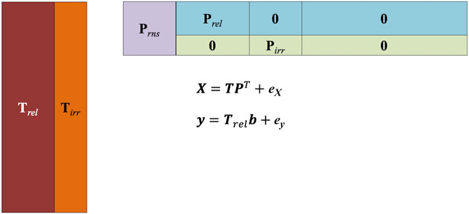
FIGURE 1. Scheme of the bilinear model used for the simulated example.

2.1.3 Selwood Data

This data set consists of 31 samples and 53 molecular descriptors (X) and the biological activity (Y) (Selwood et al., 1990). As the number of samples is small and the diversity of the descriptors for the sample is high, this data set is not evaluated by dividing the samples into a calibration and test set.

2.2 Methods

2.2.1 Multivariate Regression

There exist a number of methods for multivariate regression with latent variables. One of the most popular methods is partial least squares regression (PLSR) (Wold and Johansson, 1993; Wold et al., 2001), which has found practical use in real-time applications for quantitative prediction and quality control in chemical, agriculture, food and beverage, and pharma/biopharma over the past 30 years, to name a few applications. The model structure of PLSR is:

$\mathbf{X}={\mathbf{T}\mathbf{P}}^T+\mathbf{E},(4)$

$\mathbf{Y}={\mathbf{T}\mathbf{Q}}^T+\mathbf{F}.(5)$

The so-called loading weights are estimated as the largest eigenvector of the covariance of X and Y after deflation of A factors.

The resulting regression coefficients are estimated from the following expression:

$\widehat{\mathbf{B}}=\mathbf{W}{\left({\mathbf{P}}^T\mathbf{W}\right)}^{-1}{\mathbf{Q}}^T\mathbf{Y},(6)$

Many different algorithms exist for PLSR, depending on the properties of the input data, that is, the dimensions of X and Y. The purpose of the more efficient algorithms was to estimate the eigenvectors from the smallest dimension of a covariance matrix between X and Y. Some examples are as follows:

• NIPALS, which handles missing values directly in the algorithm;

• Kernel PLS, suited for data with many more objects than X-variables;

• Wide-kernel PLS, suited for data with many more X-variables than objects;

• SIMPLS, suited for data with many more X-variables than Y-variables.

2.2.2 Multivariate Calibration—Still Not Known as a Generic Concept After 40 years?

This paragraph is intended as a retrospective look at the part of chemometrics that started with calibration of multi-channel instruments for the prediction of, for example, concentration of a chemical compound or more less-defined quality measures (octane number and viscosity). The incentive was, in many cases, to reduce the amount of work to acquire reference (wet chemistry lab) data to a minimum and for deployment in instruments for online purposes. For some applications, for example, the production of glue, the value of the property of interest, measured by the reference method, might be available after 7 days. It is imperative that an estimate of the accuracy and precision of the reference method is acquired before starting the experimental work to build calibration models. Also, it seems that outside of the chemometrics community, it is not commonly known in natural science or included in the curriculum at universities that selectivity is not required to build models for quantification or classification. For instance, acquiring mass-spectra with a resolution of 0.0001 m/Z might be counter-productive as the columns may not be directly comparable due to small shifts of the signals along the m/Z axis. Furthermore, there is also no need to integrate peaks in chromatographic systems, assuming aligned peaks between samples (if not the case, some kind of correlation-optimized warping might be applied).

Assuming that three compounds with overlapping peaks are mixed in a solvent with zero intensity, the theory (and practice) of multivariate calibration tells us that only three variables are needed for “unmixing” this system. In principle, one only needs as many variables as there are underlying systematic structures in the data to establish a model with the optimal prediction ability. However, as there might be other sources of variation in the data such as baseline and scatter effects, the complexity of the data might be higher.

2.3 Variable Selection

Various methods for variable selection have been published and evaluated over the past decades. In particular, there are reviews or tutorial articles either focusing on one specific approach or comparing different methods (Höskuldsson, 2001; Chong and June 2005; Roy and Roy, 2008; Andersen and Bro, 2010; Mehmood et al., 2012; Liland et al., 2013; Anzanello and Fogliatto, 2014; Wang et al., 2014; Wang et al., 2015; Biancolillo et al., 2016; Mehmood et al., 2020). In this study, we focus on the variable selection with three main objectives: i) to eliminate variables that are not relevant; ii) to return a small subset of variables that has the same or better prediction performance as a model with all original variables; and iii) to evaluate the consistency of the subsets found in ii) for the selected methods. Thus, we are not focusing on finding the “best” model in terms of RMSE. Many methods will give similar prediction performance, assuming the models are validated correctly. Depending on the application, variable selection might give a lower prediction error than a model on all variables, but this is not a general conclusion for a given data set.

The methods applied for removing all non-important variables were a) significance from cross model validation (CMV), b) truncation based on t-distribution of the regression coefficients (sparse-PLS), c) variable importance for projection (VIP), d) unimportant variable elimination (UVE), and e) selectivity ratio (SR).

As a second step with the objective of evaluating if a smaller subset of variables has the same or improved prediction ability, the following approaches were chosen: i) Lasso regression, ii) best combination search or forward selection based on CMV, iii) covariance selection (CovSel), iv) applying Kennard–Stone algorithm in the variable space (K–S), v) genetic algorithms (GA), vi) selectivity ratio (SR), and vii) significant multivariate correlation (SMC).

2.3.1 Multiple Linear Regression and Regularization

One common regression method is multiple linear regression (MLR). The assumption in MLR is that there are no errors in X, which in most practical applications is not the case. Also, MLR requires more samples than variables, which in the chemometrics tradition with multi-channel instruments with hundreds of variables and few samples is not fulfilled. Therefore, many publications on MLR make use of various methods for variable selection such as forward selection, backward elimination, and stepwise selection. Common stopping rules are p-values for a given cut-off or Akaike’s information criterion (AIC) (Akaike, 1974). It is also well known that in the case of collinearity of the columns in X, including or removing a variable may change the size, sign, and p-value for other variables in the model (Tibshirani, 1996). This is conceptually not satisfactory and may lead to an erroneous interpretation of the model. It is only for orthogonal columns in X, for example, for strict orthogonal designs, that there is a unique way to estimate the sum of squares as the basis for the analysis of variance (ANOVA). The so-called embedded methods introduce a regularization parameter to cope with the challenges mentioned previously. Least absolute shrinkage and selection operator regression (Lasso) (Tibshirani, 1996) applies a shrinkage parameter λ with the purpose of producing simpler models, that is, with a (small) subset of the original variables. When λ increases, many coefficients are set to 0. At the same time, the bias increases and the variance decreases, according to the bias–variance trade-off. The optimal value for λ is typically found by cross-validation or bootstrapping. The criterion is to minimize the expression:

$\sum _{i=1}^n{\left(y_i-\sum _{j=1}^k{x}_{ij}{\beta }_j\right)}^2+\lambda \sum _{i=1}^k|{\beta }_j|.(7)$

Some review articles on MLR in combination with variable selection and Lasso are given in Heinze et al. (2018); Sauerbrei et al. (2020); and Variyath and Brobbey (2020). The use of these methods with proper validation procedures will, in general, give predictive ability similar to methods based on latent variables such as PLSR. When only a small subset of variables is included, the optimal number of factors in PLS regression might correspond to its maximum possible value, that is, a full rank model (the MLR solution). Nevertheless, a distinction between MLR-based and latent variable regression methods is that for the latter, there is no explicit need to remove variables due to k > n or high collinearity. If a variable is indirectly highly correlated with y, the causal variable might not be among the ones in the selected subset. For instance, let us assume that a model for the degree of cirrhosis is f (age, male/female, and alcohol consumption). Then, since men in general drink more than women, the binary variable male/female might be included but not alcohol consumption when applying a stepwise procedure.

2.3.2 Variable Importance for Projection

The VIP method (Wold and Johansson, 1993; Favilla et al., 2013; Tran et al., 2014) returns a ranked list of variables based on weight v_j that represents the importance in the PLS projection. The weights are measures of the contribution according to the variance explained by each PLS component where ${(w_{aj}/\Vert w_a\Vert )}^2$ represents the importance of the j variable. Since the variance explained by each component can be computed by the expression $q_a^2{t}_a^{\prime }ta$, v_j is calculated as follows:

$v_j=\sqrt{p\frac{{\sum }_{a=1}^A\left[\left(q_a^2{t}_a^{\prime }{t}_a\right){\left(w_{aj}/\Vert w_a\Vert \right)}^2\right]}{{\sum }_{a=1}^A\left(q_a^2{t}_a^{\prime }{t}_a\right)}}.(8)$

2.3.3 Covariance Selection

Covariance selection (Roger et al., 2011) exploits the principle of maximizing the covariance between the predictors and the responses which characterizes PLS regression, translating it to the variable selection context. Indeed, the CovSel algorithm could be thought of as a PLS regression in which the weights are forced to be either zero or one. More in detail, CovSel is based on an iterative procedure in which the variable having the maximum squared covariance with the response is selected:

$J_{\mathit{sel}}={\mathrm{a}\mathrm{r}\mathrm{g}\mathrm{m}\mathrm{a}\mathrm{x}}_{\mathit{j}}\Vert {\mathbf{x}}_j^T\mathbf{y}{\Vert }^2.(9)$

Then, both X and y are deflated from the contribution of the selected variable, and the procedure is repeated until a stopping criterion is met.

2.3.4 Uninformative Variable Elimination

The UVE (Centner et al., 1996) method is based on adding many random variables as the same size of X to the existing set of variables. Thereby, the estimation of the impact of noise in the model can be established, and thus the non-informative variables in the original data set can be removed as they have the same characteristics as the random variables. A leave-one-out cross-validation is applied to ensure some conservatism in the procedure.

2.3.5 Genetic Algorithms

Genetic algorithm (GA) (Leardi et al., 1992; Leardi and Lupiáñez González, 1998) repeatedly selects a subset of variables from the total number of variables (e.g., 5). The terms “crossover” and “mutation” are used to illustrate the procedure of how the variables “survive” in the selection process. One useful output of GA is a list of how frequently the variables were selected in the individual models. Typically, 1,000 realizations of a small subset are chosen for the computations.

2.3.6 Selectivity Ratio

The SR (Rajalahti et al., 2009; Kvalheim, 2010; Farrés et al., 2015; Kvalheim, 2020) is based on the target projection (TP) approach. Target projection is based on a post-projection of the predictor variables onto the fitted response vector from the estimated model. This decomposition of the original predictor matrix into a latent (TP)-component and a residual component can be expressed as follows:

$\mathbf{X}={\widehat{\mathbf{X}}}_{TP}+{\mathbf{E}}_{TP}={\mathbf{t}}_{TP}{\mathbf{p}}_{TP}^T+{\mathbf{E}}_{TP},(10)$

where the target projection scores t_TP are calculated as follows:

${\mathbf{t}}_{TP}=\mathbf{X}\frac{\mathbf{b}}{\Vert \mathbf{b}\Vert }=\frac{\widehat{\mathbf{y}}}{\Vert \mathbf{b}\Vert }.(11)$

The TP loadings from this model, which are calculated as:

${\mathbf{p}}_{TP}=\frac{{\mathbf{X}}^T{\mathbf{t}}_{TP}}{{\mathbf{t}}_{TP}^T{\mathbf{t}}_{TP}},(12)$

can be used as measures of how much each predictor variable contributed to the fitted response from the PLSR-model, and based on this SR, SR_j is introduced. For each variable j, the SR_j can be computed as:

$S{R}_j=\frac{V_{exp,j}}{V_{\mathit{res,j}}},(13)$

where V_exp ,j is the explained variance and V_res,j is the residual variance for variable j according to the (TP)-model.

The mean value of SR_j for all variables was used as a threshold.

2.3.7 Significant Multivariate Correlation

sMC (Tran et al., 2014) is analogous to SR but it defines the loadings for the predictive component directly in terms of the regression coefficients. Indeed, in sMC, the projection loadings p_sMC are calculated as:

${\mathbf{p}}_{\mathit{sMC}}=\frac{\mathbf{b}}{\Vert \mathbf{b}\Vert }.(14)$

On the other hand, the projection scores are defined analogously to TP:

${\mathbf{t}}_{\mathit{sMC}}=\mathbf{X}\frac{\mathbf{b}}{\Vert \mathbf{b}\Vert }=\frac{\widehat{\mathbf{y}}}{\Vert \mathbf{b}\Vert }.(15)$

Then, based on the previous equation, the predictor matrix X is decomposed as the contribution of the y-relevant component and the residuals as:

$\mathbf{X}={\widehat{\mathbf{X}}}_{\mathit{sMC}}+{\mathbf{E}}_{\mathit{sMC}}={\mathbf{t}}_{\mathit{sMC}}{\mathbf{p}}_{\mathit{sMC}}^T+{\mathbf{E}}_{\mathit{sMC}}=\frac{\widehat{\mathbf{y}}{\mathbf{b}}^T}{\Vert \mathbf{b}{\Vert }^2}+{\mathbf{E}}_{\mathit{sMC}}.(16)$

sMC is then calculated as the ratio of the variance along the jth variable explained by the sMC component to the residual variance for the same predictor:

$sM{C}_j=\frac{V_{\mathit{sMC,j}}}{V_{\mathit{res,j}}}.(17)$

The authors proposed to apply an F-test to identify variables that are statistically significant with respect to their relationship (regression) to Y. The F-distribution with degrees of freedom of 1 for the numerator and n-2 for the denominator is applied for a given significance level α. However, in the present study, consistent with the approach followed for SR and described in the previous paragraph, the mean value of sMC_j across all variables was used as a threshold.

2.3.8 Kennard–Stone Algorithm

The Kennard–Stone (K-S) (Kennard and Stone, 1969) algorithm has shown to be efficient in defining relevant subsets of objects for calibration and validation. In this context, we apply K-S as a means for removing redundancy between variables, for example, that all wavelengths in a specific peak in near-infrared spectroscopy will have predictive ability in a model. The principle of the Kennard–Stone algorithm is to find the point in the n-dimensional space, that is, furthest away from the mean, and then the next point is selected to be furthest away from the mean and the first point. The procedure continues until a specified number of points have been selected. The distance measure is typically Euclidean or Mahalanobis. In this case, Euclidean was chosen, as the loading weights are normalized to length 1.

2.3.9 Jack-Knifing and Cross Model Validation

While performing cross-validation, the estimation variance of the model parameters might be used based on the principle of jack-knifing (Bradley, 1982). The formula in the case of regression coefficients (Westad and Martens, 2000) is as follows:

$s^2\left(b_k\right)=\left(\sum _{m=1}^M{\left(b_k-b_{k_m}\right)}^2\right)\frac{\left(M-1\right)}{M},(18)$

where

s² (b_k) = estimated uncertainty variance of b_k; b_k = the regression coefficient for variable k using all objects;

$b_{k_m}$ = the regression coefficient for variable k from the model with all objects except the object(s) left out in cross-validation segment; $m\frac{M-1}{M}$ = scaling coefficient to make the estimate unbiased, where M is the number of cross-validation segments.

2.3.9.1 Cross Model Validation

It is known that when many models are tried and rejected in the case of cross-validation, it may lead to too optimistic results. This is, especially a challenge when various methods for variable selection are applied in the search for the “best” model. Cross model validation (CMV) (Stone, 1974; Anderssen et al., 2006; Westad, 2021), also known as double cross-validation, is a conservative approach for reducing the number of “false-positive” variables and for estimating figures of merit such as RMSE. When the purpose is to remove all variables that are non-important, one informative way to summarize the results from all the inner-loop models is to report the number of times the individual variable is found significant.

Combined with jack-knifing for uncertainty estimates and t-tests, the procedure is as follows:

1. Leave out some object(s).

2. Perform cross-validated PLS regression with jack-knifing and find significant variables.

3. Repeat with new object(s) left out.

4. Count the number of times a variable was found significant in 2.

5. Set a threshold, for example, 80%, and remove the remaining variables.

An illustration of CMV is shown in Figure 2.

FIGURE 2

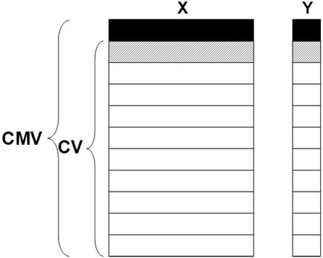
FIGURE 2. Illustration of cross model validation.

As pointed out by Westad and Marini (2015), leave-one-out (LOO) and random cross-validation schemes are not the correct levels of validation when there is (future) uncontrolled systematic variation due to stratification of the samples with respect to time, raw materials, and sensor etc. Dividing samples randomly into calibration and test set does not alleviate the danger of overfitting in this case. Yet another approach is to introduce a third level in the validation: repeated CMV (Filzmoser et al., 2009). The data sets chosen in this study did not have external information about the stratification of samples; thus, LOO and random cross-validation were the options of choice.

2.3.10 Sparse PLSR: Truncation of Variables

The idea behind sparse-PLS (Chun and Kele ş, 2010; Filzmoser et al., 2012; Liland et al., 2013) was to remove variables based on an assumed distribution of the parameters for the variables. The truncation might be applied to the loading weights w_a for each of the PLS factors or to the final B-coefficients for each variable. For the first approach, any variables kept in one or more of the factors are selected. The threshold for removing variables was set to 2, that is, at the 0.05% level.

3 Results

3.1 Results for the NIR Diesel Fuel Data

The main objectives of analyzing this data set were two-fold: i) to investigate to what extent the various methods remove all non-important variables and ii) investigate the model performance of a small subset of variables for the covariance selection, genetic algorithm, and Kennard–Stone algorithms.

The spectra were pre-processed with the Savitzky–Golay transform using the second derivative, second degree polynomial, and with 13 points.

The selected variables for the Lasso regression are marked in a plot of the mean spectrum in Figure 3. Most of the main peaks are represented, although no variables were selected in the wavelength region 1,350–1,550 nm. The optimal value of λ was found to be 0.0967.

FIGURE 3

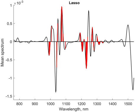
FIGURE 3. Selected variables for Lasso regression for second derivative diesel fuel spectral data.

Figure 4 shows the mean spectrum with the selected variables for CMV and sparse-PLS marked, respectively, while similar plots are shown for UVE and VIP in Figure 5. The upper plot in Figure 6 shows the selected variables for SR. Table 1 shows main results for the various methods.

FIGURE 4

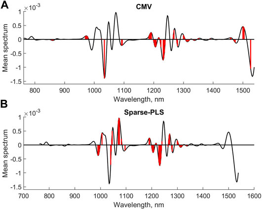
FIGURE 4. Selected variables for CMV (A) and sparse-PLS (B) for second derivative diesel fuel spectral data.

FIGURE 5

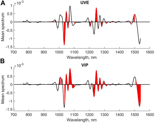
FIGURE 5. Selected variables for UVE (A) and VIP (B) for second derivative diesel fuel spectral data.

FIGURE 6

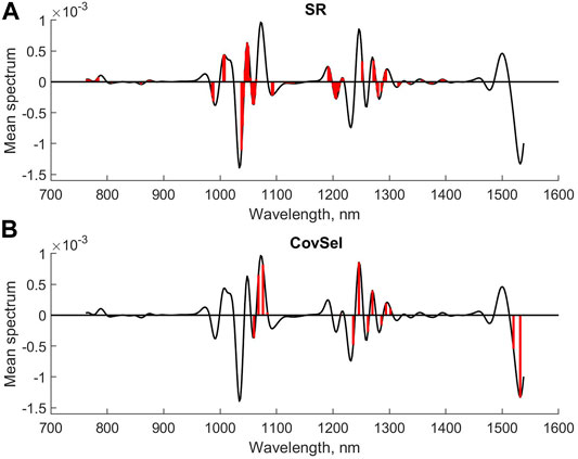
FIGURE 6. Selected variables for SR (A) and CovSel (B) for second derivative diesel fuel spectral data.

TABLE 1

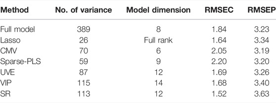
TABLE 1. Results for the diesel fuel data.

The interpretation of the results for the methods is that they, to a large extent, select one or more variables in the same main peaks in the spectra. The VIP and SR seem to be the least conservative. The sparse-PLS approach in this case simply kept the variables based on the t-distribution of the regression coefficients. The number of factors was nine for this model. The original approach was to keep all variables that are selected in one or more of the individual loading weights vector. This approach selected 163 variables and represents how PLS is compensating for non-relevant variance in X into a final regression coefficient (results not shown).

The next step in the analysis was to compare methods that are aiming for selecting a small subset of the variables. The covariance selection ended up with a subset of 15 variables, where 23 variables were kept for genetic algorithms. The number of variables for the Kennard–Stone method was preset to 15. The RMSEP values were 3.19, 3.19, and 3.22.

Figure 6 (lower plot) and Figure 7 show the selected variables for the GA, CovSel, and Kennard–Stone methods. As can be seen, there is some consistency among the variables although there are also peaks where only one of the methods has selected variables. This is not unexpected, as there exists a high degree of redundancy between the variables. Not only do variables in the individual peaks have the same relationships, but several peaks also represent the same underlying chemistry (various overtones in the NIR bands). Therefore, it is not surprising that different subsets are selected. Also, for these models, the RMSEP values are not significantly different.

FIGURE 7

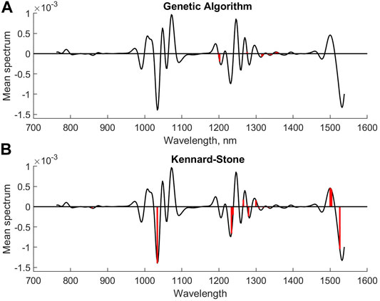
FIGURE 7. Selected variables for GA (A) and (B) K-S for second derivative diesel fuel spectral data.

3.2 Results for the Simulated Data

A summary of the results for two simulation scenarios with mean-centered data is shown in Tables 2, 3. In the second simulation, the level of the noise added to both the response and predictors was twice the noise level set in the first simulation (i.e., 10%). The ideal result for the first column is 100%, whereas 0% would be the optimal result for columns 3 and 4. For the “relevant non-selective” column, it is not so evident what the optimal result should be.

TABLE 2

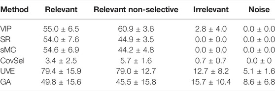
TABLE 2. Results from the analysis of the simulated data at the 5% noise level.

TABLE 3

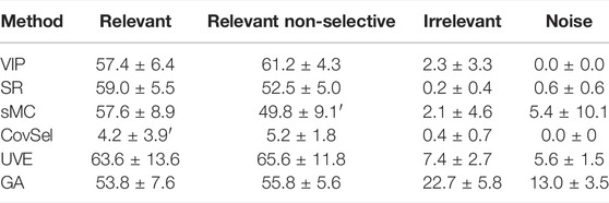
TABLE 3. Results of the analysis of the simulated data at the 10% noise level.

The tables show that GA erroneously selects more variables of irrelevant types and noise when the noise level increases. Furthermore, GA identifies a higher percentage of relevant and relevant non-selective variables. This may due to the fact that GA performs a form of the best combination search which may select noisy (spurious) variables. The UVE identifies fewer relevant and relevant non-selective variables, but at the same time, the percentage of irrelevant variables is decreasing. The selectivity ratio identifies a higher percentage of relevant and relevant non-selective variables in the presence of noise. The CovSel gives a very low percentage of relevant and relevant non-selective variables. This is as expected, as CovSel has the objective of finding a subset of non-redundant variables.

3.3 Results for the Selwood Data

The existing literature reports various combinations of five variables for a model with the highest validated explained variance. The best combination search procedure with the sorted p-values from jack-knifing estimates was used as a reference. When no improvement in the RMSE for cross-validation was achieved, the search was stopped. The procedure returned variables 4, 12, 39, 50, and 52 as the optimal set. This gave an $R_{\mathit{Cal}}^2$ of 72% and an $R_{\mathit{V\; al}}^2$ of 64% after four factors, which is similar to the results reported in the literature. Nevertheless, as there are only 31 samples and no independent test set, the search for the lowest explained variance or RMSE is not the main objective in this context, and such a procedure may lead to overfitting. As there is redundancy among many variables, there are many combinations of five variables that will yield the same results.

Table 4 gives an overview of the top five selected variables for various methods.

TABLE 4

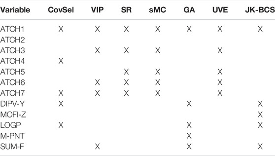
TABLE 4. Selected variables for various methods for the Selwood data.

The results show a large degree of consistency among the methods. The methods based on univariate measures seem to select very similar subsets, whereas methods that search for different combinations showed more diverse subsets within the multivariate space. All methods identified the variable with the highest correlation to the first factor in the PLS model.

Many of the variables represent the same underlying structure of the data, so depending on the strategy, the subset which is found might be more or less random. However, there is no need to remove variables in multivariate regression methods such as PLSR. The variables that are removed can be visualized by use of correlation loadings, which are the square root of the explained variance per factor and variable. Figure 8 shows the correlation loadings for the first two factors from the five variables selected in the JK-BCS, whereas the other variables selected in Table 2 are downweighted and marked in green. Thus, the variables that were not included in the selected subset are visualized, and their relation to the other variables can be interpreted. Thereby, in cases where there are indirect correlations between causal variables and variables selected by a given procedure, the interpretation regarding causality is not (accidentally) lost due to the method of choice. From the figure, it can be interpreted that all variables with the name “ATCH” except ATCH2 and ATCH4 have similar relations to activity (correlations between 0.54 and 0.60). This is probably why GA and JK-BCS only selected one of these, due to redundancy. ATCH2 and ATCH4 are selected by CS because these variables span another part of the model subspace (recall that the optimal number of factors is four).

FIGURE 8

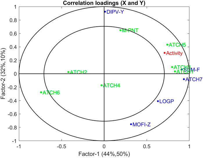
FIGURE 8. Correlation loadings with the variables not selected by JK-BCS are denoted in green and their variable activity in red.

The correlation between the individual variables and the response variable is in one method for screening non-relevant variables. However, this is, in general, not a robust strategy, although for spectroscopy it might serve as a viable approach. In this QSAR data set, the various molecules show quite different properties of the variables, which gives subgroups in the score space. In fact, the variables DIPV-Y and MOFI-Z that span factor two in the JK-BCS model have empirical correlations of 0.23 and 0.00 to Y.

4 Discussion

The analysis of the NIR diesel fuel spectra showed that various methods selected quite consistent subsets of variables with the purpose of eliminating variables that are not important. The next step, selecting a small subset, showed more variation among the methods evaluated. The methods gave the same prediction error for the test set.

The analysis of the simulated data showed that the methods identified between 50 and 80% of the relevant variables. VIP and SR had almost zero false-positives for the irrelevant and noise variables for both noise levels. sMC was more susceptible to noise than VIP and SR. UVE identified the highest percentage of relevant variables, on the cost of 5–13% false-positives. GA reported the highest percentage of false-positives. CovSel, with the objective of finding a small number of non-redundant variables, did not give false-positives but also reported a small number of relevant and relevant non-selective variables.

The comparison of the methods that aim to find a small subset of variables showed that there is a high degree of consistency in the ranking of the variables for the Selwood data. By the use of correlation loadings, interpretability is kept, as the correlations to the underlying factors can be made. Thus, if some variables are highly correlated, it does not matter from an interpretational point of view which ones are selected for a small subset. Nevertheless, it is a sound principle to remove variables that are not relevant. This reduces complexity and might also decrease the prediction error.

Two of several objectives with variable selections are: i) to eliminate variables that are not relevant and ii) to return a small subset of variables that have the same or better prediction performance as a model with all original variables. We find that these aspects are more relevant than the comparison of RMSE for a number of methods, as most methods give similar results.

5 Conclusion

In the present study, different variable selection strategies were reviewed and compared, taking into account various aspects. Based on the results obtained from real and simulated data and discussed in the previous section, some general conclusions can be drawn.

The predictive ability was not significantly different for various variable selection methods, which shows that methods with similar objectives may give the same results. It also means that, for data with redundancy among the variables, there can be many models with the same predictive ability. At the same time, it is worth stressing that there can be, as well, many cases where the use of a variable selection strategy may lead to an improvement of the model performances, as reflected in the value of one or more figures of merit.

None of the methods selected all the relevant variables, the highest percentage of relevant predictors being retained by the UVE approach (about 80% for the data with 5% noise level). At the same time, most of the approaches did not select any (or were retaining just a very small amount) of the irrelevant and noisy predictors. In this respect, only GA and, to a lesser extent, UVE, were including a relatively high amount of these “spurious” variables.

The variable selection methods that are based on some kind of search for the “best” model or representing diversity return subsets that are more diverse within the multivariate model space (GA, JK. BCS, and CovSel) than the single criterion methods.

For the methods based on latent variables, there is no need to remove variables completely: they may be downweighted so that one can have both interpretability and optimal prediction performance.

Data Availability Statement

The datasets presented in this study can be found in online repositories. The names of the repository/repositories and accession number(s) can be found at: https://eigenvector.com/wp-content/uploads/2019/06/SWRI\_Diesel\_NIR.zip, https://github.com/josecamachop/MEDA-Toolbox/tree/master/Examples/Chemometrics/Selwood.

Author Contributions

Both authors contributed to data analysis, manuscript revision, and read and approved the submitted version.

Funding

This open access publication was funded by the BRU21-NTNU Research and Innovation Program on Digital and Automation Solutions for the Oil and Gas Industry (www.ntnu.edu/bru21).

Conflict of Interest

Author FW was employed by Idletechs AS.

The remaining author declares that the research was conducted in the absence of any commercial or financial relationships that could be construed as a potential conflict of interest.

Publisher’s Note

All claims expressed in this article are solely those of the authors and do not necessarily represent those of their affiliated organizations, or those of the publisher, the editors, and the reviewers. Any product that may be evaluated in this article, or claim that may be made by its manufacturer, is not guaranteed or endorsed by the publisher.

References

Akaike, H. (1974). A New Look at the Statistical Model Identification. IEEE Trans. Autom. Contr. 19 (6), 716–723. doi:10.1109/tac.1974.1100705

CrossRef Full Text | Google Scholar

Andersen, C. M., and Bro, R. (2010). Variable Selection in Regression-A Tutorial. J. Chemom. 24 (11-12), 728–737. doi:10.1002/cem.1360

CrossRef Full Text | Google Scholar

Anderssen, E., Dyrstad, K., Westad, F., and Martens, H. (2006). Reducing Over-optimism in Variable Selection by Cross-Model Validation. Chemom. Intell. Lab. Syst. 84 (1-2), 69–74. doi:10.1016/j.chemolab.2006.04.021

CrossRef Full Text | Google Scholar

Anzanello, M. J., and Fogliatto, F. S. (2014). A Review of Recent Variable Selection Methods in Industrial and Chemometrics Applications. Eur. J. Industr. Eng. 8 (5), 619. doi:10.1504/ejie.2014.065731

CrossRef Full Text | Google Scholar

Biancolillo, A., Liland, K. H., Måge, I., Næs, T., and Bro, R. (2016). Variable Selection in Multi-Block Regression. Chemom. Intell. Lab. Syst. 156, 89–101. doi:10.1016/j.chemolab.2016.05.016

CrossRef Full Text | Google Scholar

Bradley, E. (1982). “The Jackknife, the Bootstrap and Other Resampling Plans,” in CBMS-NSF Regional Conference Series in Applied Mathematics (Philadelphia, PA: SIAMLectures Given at Bowling Green State Univ). Available at: https://cds.cern.ch/record/98913.

Google Scholar

Centner, V., Massart, D.-L., de Noord, O. E., de Jong, S., Vandeginste, B. M., and Sterna, C. (1996). Elimination of Uninformative Variables for Multivariate Calibration. Anal. Chem. 68 (21), 3851–3858. doi:10.1021/ac960321m

PubMed Abstract | CrossRef Full Text | Google Scholar

Chong, I.-G., and Jun, C.-H. (2005). Performance of Some Variable Selection Methods when Multicollinearity Is Present. Chemom. Intell. Lab. Syst. 78 (1-2), 103–112. doi:10.1016/j.chemolab.2004.12.011

CrossRef Full Text | Google Scholar

Chun, H., and Keleş, S. (2010). Sparse Partial Least Squares Regression for Simultaneous Dimension Reduction and Variable Selection. J. R. Stat. Soc. Ser. B (Statistical Methodology) 72 (1), 3–25. doi:10.1111/j.1467-9868.2009.00723.x

CrossRef Full Text | Google Scholar

Farrés, M., Platikanov, S., Tsakovski, S., and Tauler, R. (2015). Comparison of the Variable Importance in Projection (VIP) and of the Selectivity Ratio (SR) Methods for Variable Selection and Interpretation. J. Chemom. 29 (10), 528–536. doi:10.1002/cem.2736

CrossRef Full Text | Google Scholar

Favilla, S., Durante, C., Vigni, M. L., and Cocchi, M. (2013). Assessing Feature Relevance in NPLS Models by VIP. Chemom. Intell. Lab. Syst. 129, 76–86. doi:10.1016/j.chemolab.2013.05.013

CrossRef Full Text | Google Scholar

Filzmoser, P., Gschwandtner, M., and Todorov, V. (2012). Review of Sparse Methods in Regression and Classification with Application to Chemometrics. J. Chemom. 26 (3-4), 42–51. doi:10.1002/cem.1418

CrossRef Full Text | Google Scholar

Filzmoser, P., Liebmann, B., and Varmuza, K. (2009). Repeated Double Cross Validation. J. Chemom. 23 (4), 160–171. doi:10.1002/cem.1225

CrossRef Full Text | Google Scholar

Heinze, G., Wallisch, C., and Dunkler, D. (2018). Variable Selection - a Review and Recommendations for the Practicing Statistician. Biom. J. 60 (3), 431–449. doi:10.1002/bimj.201700067

PubMed Abstract | CrossRef Full Text | Google Scholar

Höskuldsson, A. (2001). Variable and Subset Selection in PLS Regression. Chemom. Intell. Lab. Syst. 55 (1-2), 23–38. doi:10.1016/s0169-7439(00)00113-1

CrossRef Full Text | Google Scholar

Kennard, R. W., and Stone, L. A. (1969). Computer Aided Design of Experiments. Technometrics 11 (1), 137–148. doi:10.1080/00401706.1969.10490666

CrossRef Full Text | Google Scholar

Kvalheim, O. M. (2010). Interpretation of Partial Least Squares Regression Models by Means of Target Projection and Selectivity Ratio Plots. J. Chemom. 24 (7-8), 496–504. doi:10.1002/cem.1289

CrossRef Full Text | Google Scholar

Kvalheim, O. M. (2020). Variable Importance: Comparison of Selectivity Ratio and Significance Multivariate Correlation for Interpretation of Latent‐variable Regression Models. J. Chemom. 34 (4), e3211. doi:10.1002/cem.3211

CrossRef Full Text | Google Scholar

Leardi, R., Boggia, R., and Terrile, M. (1992). Genetic Algorithms as a Strategy for Feature Selection. J. Chemom. 6 (5), 267–281. doi:10.1002/cem.1180060506

CrossRef Full Text | Google Scholar

Leardi, R., and Lupiáñez González, A. (1998). Genetic Algorithms Applied to Feature Selection in PLS Regression: How and when to Use Them. Chemom. Intell. Lab. Syst. 41 (2), 195–207. doi:10.1016/s0169-7439(98)00051-3

CrossRef Full Text | Google Scholar

Liland, K. H., Høy, M., Martens, H., and Sæbø, S. (2013). Distribution Based Truncation for Variable Selection in Subspace Methods for Multivariate Regression. Chemom. Intell. Lab. Syst. 122, 103–111. doi:10.1016/j.chemolab.2013.01.008

CrossRef Full Text | Google Scholar

Mehmood, T., Liland, K. H., Snipen, L., and Sæbø, S. (2012). A Review of Variable Selection Methods in Partial Least Squares Regression. Chemom. Intell. Lab. Syst. 118, 62–69. doi:10.1016/j.chemolab.2012.07.010

CrossRef Full Text | Google Scholar

Mehmood, T., Sæbø, S., and Liland, K. H. (2020). Comparison of Variable Selection Methods in Partial Least Squares Regression. J. Chemom. 34 (6), e3226. doi:10.1002/cem.3226

CrossRef Full Text | Google Scholar

Rajalahti, T., Arneberg, R., Berven, F. S., Myhr, K.-M., Ulvik, R. J., and Kvalheim, O. M. (2009). Biomarker Discovery in Mass Spectral Profiles by Means of Selectivity Ratio Plot. Chemom. Intell. Lab. Syst. 95 (1), 35–48. doi:10.1016/j.chemolab.2008.08.004

CrossRef Full Text | Google Scholar

Roger, J. M., Palagos, B., Bertrand, D., and Fernandez-Ahumada, E. (2011). CovSel: Variable Selection for Highly Multivariate and Multi-Response Calibration. Chemom. Intell. Lab. Syst. 106 (2), 216–223. doi:10.1016/j.chemolab.2010.10.003

CrossRef Full Text | Google Scholar

Roy, P. P., and Roy, K. (2008). On Some Aspects of Variable Selection for Partial Least Squares Regression Models. QSAR Comb. Sci. 27 (3), 302–313. doi:10.1002/qsar.200710043

CrossRef Full Text | Google Scholar

Sauerbrei, W., Perperoglou, A., Schmid, M., Abrahamowicz, M., Becher, H., Binder, H., et al. (2020). State of the Art in Selection of Variables and Functional Forms in Multivariable Analysis-Outstanding Issues. Diagn Progn. Res. 4 (1), 3. doi:10.1186/s41512-020-00074-3

PubMed Abstract | CrossRef Full Text | Google Scholar

Selwood, D. L., Livingstone, D. J., Comley, J. C. W., O'Dowd, A. B., Hudson, A. T., Jackson, P., et al. (1990). Structure-activity Relationships of Antifilarial Antimycin Analogs: A Multivariate Pattern Recognition Study. J. Med. Chem. 33 (1), 136–142. doi:10.1021/jm00163a023

PubMed Abstract | CrossRef Full Text | Google Scholar

Stone, M. (1974). Cross-Validatory Choice and Assessment of Statistical Predictions. J. R. Stat. Soc. Ser. B Methodol. 36 (2), 111–133. doi:10.1111/j.2517-6161.1974.tb00994.x

CrossRef Full Text | Google Scholar

Tibshirani, R. (1996). Regression Shrinkage and Selection via the Lasso. J. R. Stat. Soc. Ser. B Methodol. 58 (1), 267–288. doi:10.1111/j.2517-6161.1996.tb02080.x

CrossRef Full Text | Google Scholar

Tran, T. N., Afanador, N. L., Buydens, L. M. C., and Blanchet, L. (2014). Interpretation of Variable Importance in Partial Least Squares with Significance Multivariate Correlation (sMC). Chemom. Intell. Lab. Syst. 138, 153–160. doi:10.1016/j.chemolab.2014.08.005

CrossRef Full Text | Google Scholar

Variyath, A. M., and Brobbey, A. (2020). Variable Selection in Multivariate Multiple Regression. PLoS One 15 (7), e0236067. doi:10.1371/journal.pone.0236067

PubMed Abstract | CrossRef Full Text | Google Scholar

Wang, Z. X., He, Q. P., and Wang, J. (2015). Comparison of Variable Selection Methods for PLS-Based Soft Sensor Modeling. J. Process Control 26, 56–72. doi:10.1016/j.jprocont.2015.01.003

CrossRef Full Text | Google Scholar

Wang, Z. X., He, Q., and Wang, J. (2014). “Comparison of Different Variable Selection Methods for Partial Least Squares Soft Sensor Development,” in 2014 American Control Conference, Portland, OR, USA, 4-6 June 2014 (IEEE). doi:10.1109/acc.2014.6859335

CrossRef Full Text | Google Scholar

Westad, F. (2021). A Retrospective Look at Cross Model Validation and its Applicability in Vibrational Spectroscopy. Spectrochimica Acta Part A Mol. Biomol. Spectrosc. 255, 119676. doi:10.1016/j.saa.2021.119676

CrossRef Full Text | Google Scholar

Westad, F., and Marini, F. (2015). Validation of Chemometric Models - A Tutorial. Anal. Chim. Acta 893 (14–24), 14–24. doi:10.1016/j.aca.2015.06.056

PubMed Abstract | CrossRef Full Text | Google Scholar

Westad, F., and Martens, H. (2000). Variable Selection in Near Infrared Spectroscopy Based on Significance Testing in Partial Least Squares Regression. J. Near Infrared Spectrosc. 8 (2), 117–124. doi:10.1255/jnirs.271

CrossRef Full Text | Google Scholar

Wold, M. C. S., and Johansson, Erik. (1993). “3D QSAR in Drug Design: Theory, Methods and Applications,” in Chapter PLS: Partial Least Squares Projections to Latent Structures (Leiden, ESCOM Science Publishers), 523–550.

Google Scholar

Wold, S., Sjöström, M., and Eriksson, L. (2001). PLS-Regression: A Basic Tool of Chemometrics. Chemom. Intell. Lab. Syst. 58 (2), 109–130. doi:10.1016/s0169-7439(01)00155-1

CrossRef Full Text | Google Scholar