Automated approaches for the early stage distinguishing of Palmer amaranth from waterhemp

Palmer amaranth and waterhemp are two invasive pigweed species, which have become most troublesome to crops, especially corn and soybean. Among these two weed species, Palmer amaranth is more harmful to crops as it can grow faster, spread rapidly, and reduce crop yields significantly when compared to waterhemp. Distinguishing Palmer amaranth from waterhemp is important for effective weed management and an increase in crop production. However, differentiating these two weeds in the early stage is considerably difficult owing to their similar morphological characteristics. In the current study, three artificial intelligence approaches, namely machine learning (ML), deep learning (DL), and object detection (OD) were employed to automate the identification of greenhouse-grown Palmer amaranth and waterhemp within two weeks after emergence, from their RGB images. Aspect ratio, roundness, and circularity were measured and supplied as the input for the ML classification models. Among the four ML models employed, the random forest model achieved the top classification accuracy of 70% with only 312 training instances. In the case of deep learning, the proposed convolutional neural network model trained on a single-object RGB image of Palmer amaranth and waterhemp achieved a classification accuracy of 93%, outperforming the top ML model. The image dataset used for the DL model increased from the original size of 2,000 to 16,000 by various augmentation techniques. Finally, a transfer-learning-based object detection model for localized identification of the weeds was designed. The OD model was developed by fine-tuning the head of YOLOv5 trained on the COCO dataset with 3,200 single-object images (images with single foliage of either Palmer amaranth or waterhemp). The OD model developed in this study achieved an accuracy of 83.5% and it can identify the weed foliages irrespective of their size and proximity to each other.

1 Introduction

Palmer amaranth (Amaranthus palmeri) and waterhemp (Amaranthus tuberculatus) are two invasive pigweed species (Bradley et al., 2022; Roberts and Florentine, 2022) that pose severe threats to the productivity of several row crops, especially corn and soybean (Massinga et al., 2001; Bensch et al., 2003; Steckel and Sprague, 2004). Both these weeds are characterized by rapid growth under ideal growing conditions (Bradley et al., 2022; Roberts and Florentine, 2022). They compete with crops for essential resources (light, water, and nutrients) and cause a drastic reduction in their yields (Berger et al., 2015; Butts et al., 2018; Mahoney et al., 2021). However, Palmer amaranth is known to be more aggressive than waterhemp for several reasons. Palmer amaranth can grow at a faster rate than waterhemp, for an instance, a study conducted by Perkins et al. records a growth rate of 55 mm per day for Palmer amaranth and a growth rate of 44mm per day for waterhemp in untreated cover crops (Perkins et al., 2021). Furthermore, amaranth species demonstrate a greater ability to disperse across the fields owing to their smaller seed size, resulting in a wider infestation of crop fields. Moreover, herbicide-resistant Palmer amaranth biotypes are commonplace. Jonathon and Christy (Kohrt and Sprague, 2017) reported Palmer amaranth is resistant to six herbicide sites of action, including glyphosate. Chahal et al (2015) reported Palmer amaranth is one of the very few weeds in the United States to have evolved resistance to herbicide groups with multiple mechanisms of action including 5-enol-pyruvylshikimate-3-phosphate synthase inhibitors (EPSPS), microtubule assembly inhibitors, acetolactate synthase inhibitors (ALS), hydroxyphenylpyruvate dioxygenase inhibitors (HPPD) and photosystem (PS) II inhibitors (Heap, 2020). These arguments indicate the need for distinguishing Palmar amaranth from waterhemp for effective weed management.

Fully grown Palmer amaranth can be manually differentiated from waterhemp through its morphological characteristics such as leaf shape, petiole length, presence of a watermark, presence of leaf tip hair, and presence of bracts (Ikley and Jenks, 2019). A comparison of morphological characteristics between Palmer amaranth and waterhemp is described in detail in Table 1. Though extensive research has been done on their plant morphologies for their identification (Trucco et al., 2006; Molin and Nandula, 2017), studies that utilize machine learning and deep learning techniques to distinguish them in the field at a large scale are lacking. Also, these distinct differences observed in their morphology are absent in the early stages of their growth (within two weeks after emergence) and the striking resemblance of Palmer amaranth to waterhemp at the early stages poses a considerable challenge in the identification of individual weeds. Alternatively, genetic testing can be used reliably at the early stage (Montgomery et al., 2019). Genetic testing involves collecting the weed seed samples, performing genomic sequencing on them, searching for specific genetic differences, and designing genetic markers to distinguish Palmer amaranth from the other species based on DNA (Jiang and Köhler, 2012). However, the process of genetic testing (both leaf tissue testing and seed sample testing) is expensive and also a laborious process that involves manual intervention at several stages of the testing. Hence, the goal of this study is to distinguish Palmer amaranth from waterhemp at its early stages (in the first two weeks after emergence) using automated approaches such as machine learning, deep learning, and object detection techniques.

Table 1

Table 1. Morphological characteristics of Palmer amaranth and waterhemp.

We hypothesize that it is possible to distinguish Palmer amaranth from waterhemp in the early stages after emergence automatically employing image data alone. The overall objective of this study is to train machine learning, deep learning and localized detection methods employing image data to automatically distinguish Palmer amaranth from waterhemp in the early stages. To this end several machine learning methods and a deep learning approach are employed for distinguishing Palmer amaranth from waterhemp using leaf features and RGB images, respectively. In addition, an object model is trained for locaFlized identification of the weeds in images mixed with both weed foliage. While early detection of Palmer amaranth is very advantageous in itself, the proposed methods can serve as diagnostic methods before more elaborate and time-taking detection procedures such as genetic testing are resorted to. Despite this, the proposed methods are highly dependent on the fidelity of the training data and quality of the images used for classification of the weeds.

The rest of the manuscript is organized as follows: Section 2 briefs the overall research approach used in the study; Section 3 discusses the process of acquiring the weed images and the pre-processing involved; Section 4 describes the analysis of leaf geometrical parameters; Section 5, 6 and 7 discusses the model details and result obtained from machine learning, deep learning and object detection methods, respectively; Section 8 summarizes the conclusions drawn from the study; and finally, Section 9 details the limitations and future research direction of the current study.

2 Overall study approach

The current study focuses on implementing three important automated tasks for weed management and analyzing the performance of the implemented models. The three automated tasks are 1. Classification of the two weed species (Palmer amaranth and waterhemp) by employing popular machine learning methods 2. Classification of the two weed species using a deep learning approach, and 3. Identification of individual weeds in an image using a state-of-the-art object detection technique. The study process starts with acquiring images of Palmer amaranth and waterhemp plants in a laboratory setting. The acquired images are preprocessed subsequently to eliminate trivial features and are suitable for training the AI (artificial intelligence) models. The leaf features are then extracted from the processed images and the distribution of the leaf features is analyzed. Afterward, the machine learning models are trained to classify the two weed species with the use of the extracted leaf features from the preprocessed images followed by the training of a deep learning model by using the images directly. The performance of the models is analyzed and compared subsequently. Finally, using transfer learning, an object detection model is trained with the images containing a random mixture of Palmer amaranth and waterhemp plants. The methodology employed in this study is presented in Figure 1.

Figure 1

Figure 1. Illustration of study methodology employed in this work.

3 Research methods

3.1 Methods for data collection and preprocessing

The data collection process for this study involves capturing images of the two target weed species: Palmer amaranth (PA) and waterhemp (WH). Seeds of both species were obtained in separate packages, and genetic testing was performed prior to planting to verify species identity. Fifty plants of each species were grown in pots in a controlled greenhouse environment at North Dakota State University (NDSU), Fargo, ND. To prevent any mixing of species during growth and data collection, Palmer amaranth and waterhemp plants were grown in separate designated areas of the greenhouse, with permanent floor markers indicating species label.

The pots were continually irrigated under controlled conditions, and image acquisition was performed using a high-resolution camera (24.2 MP Canon EOS Rebel T7i DSLR, equipped with an EF-S 18-55mm f/4-5.6 IS STM lens) established on a stable platform, with the lens focused normally to the leveled soil surface of a pot. Images were taken under controlled lighting conditions, with the greenhouse lights turned off to prevent interference with the imaging process. Care was also taken to ensure the plants’ growth was not impeded or harmed during the image-acquiring process.

To ensure accurate data labeling and prevent any mixing of images between species, the image acquisition was conducted sequentially - completing all images for one species before moving to the next. During image acquisition, a temporary identification sheet displaying the species name was placed within each image frame for later corroboration. Images were acquired daily from the day of emergence between 1:00 p.m. to 3:00 p.m. and were captured at three different heights: 5 cm, 10 cm, and 20 cm from the soil surface, maintaining a 90-degree angle to the pot soil surface. The details of the experimental setup are provided in Table 2. A total of 2,000 images were acquired: 1,000 images each of Palmer amaranth and water hemp. The raw images were captured in RAW format and converted to JPEG, consisting of three channels (red, green, and blue) with a resolution of 4020 × 6024 pixels. The acquired images underwent preprocessing for training the classification and object identification models. The preprocessing protocol involved the systematic removal of secondary features such as pot area, dead leaves, soil background, and the temporary identification sheets using the Image Segmenter tool in MATLAB. The final preprocessed images consist only of plants against a black background, as illustrated in Figure 2.

Table 2

Table 2. Details of the experiment conducted for image acquisition.

Figure 2

Figure 2. (A) Original image of weed foliage, and (B) image after removing the extraneous features.

3.2 Methods for assessing the accuracy of the classification models

This study utilizes five key metrics to evaluate the performance of the artificial intelligence (AI) models: 1) classification accuracy, 2) confusion matrix, 3) precision, 4) recall, and 5) F₁-score. For the classification models, accuracy is reported for the overall dataset, while confusion matric, precision, recall, and F₁-score are applied to assess class-wise performance. In contrast, for the object detection model, only classification accuracy is used, but it is also evaluated on a per-class basis. The details of these metrics are explained below. Classification accuracy is the ratio of the number of correctly classified instances to the number of total testing instances. Confusion matrix is an important performance metric after classification accuracy. It is a contingency table that summarizes (as counts or proportions) correct and incorrect classifications of the data instances of the individual classes. The rows of the confusion matrix correspond to true classes and the columns of the confusion matrix correspond to the predicted classes. The size of the confusion matrix is $n_c \times n_c$. Here, $n_c$ denotes the number of class labels, in our case, $n_c=2$ as the class labels are two: ‘$PA$’ (Palmer amaranth) and ‘$WH$‘ (Waterhemp). The diagonal elements of the confusion matrix record the correctly classified instances of each class and off-diagonal elements record the instances of each class misclassified into other classes. Figure 3A shows an illustrative confusion matrix used in this study. ‘$PP$’, ‘$PW$’, ‘$WP$’, ‘$WW$’ are shown as the entries of this confusion matrix. The first script of an entry signifies the true class, and the second script signifies the predicted class. For example, ‘$WP$’ represents the instances that belong to the waterhemp ($W$) class classified into the Palmer amaranth ($P$) class. Precision, Recall, and F₁-score are determined using the entries of the confusion matrix. These three metrics are computed class-wise (individually for each class) using the expressions given in Table 3. Precision is the ratio of the number of correctly predicted instances of a class to the total number of predictions made in that class. Recall is the ratio of the number of correctly predicted instances of a class to the total number of instances in that class. Precision measures the preciseness of the class predictions whereas Recall measures the extent to which true instances of a class are identified. F₁-score combines both these metrics, and it is a harmonic mean of Precision and Recall.

Figure 3

Figure 3. (A) Illustrative confusion matrix for the classification of Palmer amaranth (PA) and waterhemp (WH). The first letter of a label inside a matrix cell signifies the true category and the second letter on the label signifies the predicted category. (B) Confusion matrices of the ML models: 1. Random Forest (RF), 2. Support Vector Machine (SVM), 3. Logistic Regression (LR), and 4. K-nearest neighbors (KNN) employed for the classification of PA and WH. The diagonal elements of the confusion matrices show the counts of correctly classified instances, and the off-diagonal elements show the counts of misclassified instances.

Table 3

Table 3. Expressions to compute class-wise performance metrics.

4 Results and discussion

4.1 Classification of Palmer amaranth and waterhemp using machine learning approach

Machine learning (ML) models are computer algorithms that can make decisions or predictions by implicitly learning from the data fed to them. ML approaches are less data-intense and thus suitable when the predictions are to be made with a small amount of data (Mahesh, 2020). Accordingly, ML approaches demand less computational overhead and take a smaller training period. In our current study, four popular machine learning approaches namely support vector machines (SVM), k-nearest neighbors (KNN), random forest (RF), and logistic regression (LR) are employed to classify palmer amaranth and waterhemp. The training of these machine learning models begins with data generation through feature extraction, followed by the preparation of a structured (tabular) dataset, configuration of the classification models, and subsequent performance analysis.

4.2 Data generation for machine learning approach

The dataset that is required to train machine learning models for the classification of Palmer amaranth and waterhemp involves two steps: 1. Extracting geometrical features of the weed species from leaf images, and 2. Compute non-dimensional input features (predictors). The geometrical parameters were obtained from the preprocessed images of Palmer amaranth and waterhemp leaves were captured from Day 8 to Day 14 after emergence (refer to Section 3). A total of 36 individual leaves from each species were randomly selected, yielding 312 total observations (156 for each species). Leaf images with distortions were excluded from the analysis to ensure accurate measurements. Leaf geometrical parameters namely length ($L$), breadth ($B$), perimeter ($P$), and area ($A$) were measured from the preprocessed images of each weed species (Palmer amaranth and waterhemp) using ImageJ software. Length ($L$) was measured along the petiole axis (major axis) of the leaf, while the breadth ($B$) was measured perpendicular to the major axis. Perimeter ($P$), and area ($A$) are obtained by tracing a curve along the leaf boundary. The geometrical parameters were then used to compute dimensionless quantities, including aspect ratio ($\theta$), circularity ($\psi$), and roundness ($\mathcal{R}$), using the formulas outlined in Table 4. These dimensionless features were selected as input predictors for the machine learning models because previous studies (Aakif and Khan, 2015; Salve et al., 2016; Elnemr, 2017) have demonstrated that they effectively capture the essential discriminatory information from the raw geometrical parameters. Furthermore, the use of dimensionless parameters ensures that the features are unaffected by image magnification, providing consistency across different image scales. Additionally, using a smaller number of features allows the machine learning models to learn more efficiently, often requiring fewer examples to identify the underlying patterns.

Table 4

Table 4. Expressions to compute dimensionless leaf quantities.

4.3 Dataset preparation for machine learning approach

A tabular dataset was then prepared with these dimensionless leaf geometrical quantities as input features (predictors) from 312 data instances equally divided between the two weed species. The tabular dataset, $D_1$, consists of a feature array, $X_1\in {ℝ}^{n\times m}$, and a label vector, $Y_1\in {ℝ}^{n\times 1}$, where $n$ is the number of data instances and $m$ is the number of input features. In the current case, $n$ and $m$ are $312$ and $3$ respectively. A $k$th row of the feature array is defined as $x^{(k)}=(x_{1,}^{(k)}\cdots ,x_m^{(k)})$, where $x_{1,}^{(k)}\text{...},x_m^{(k)}$ are the input features and $k$ ranges from $1$ to $n$. The tabular dataset is divided into training ($D_{1,tn}$) and testing ($D_{1, tt}$) dataset with a 70:30 split ratio. Afterward, the ML models employed in the study are trained with the training dataset, $D_{tn}$. The performances of the models are then evaluated with the testing dataset, $D_{tt}$ using metrics such as classification accuracy, confusion matrix, precision, recall, and F1-score (Naser and Alavi, 2021).

4.4 Preliminary data analysis on the extracted data

Before applying machine learning models for classification, preliminary data analysis was conducted to examine the evolution of the dimensionless geometric quantities for each weed species. This analysis aimed to understand how the input features (predictors) – aspect ratio ($\theta$), circularity ($\psi$), and roundness ($R$)—change over time after emergence for both Palmer amaranth and waterhemp. The evolution of mean values of these quantities from Day 8 to Day 14 after emergence were plotted in Figure 4. The mean aspect ratios of Palmer amaranth and waterhemp plotted in Figure 4A exhibit an overall downward trend over the days of growth. The mean aspect ratio of Palmer amaranth gradually falls from 3.01(day 8) to 2.74 (day 14) whereas waterhemp falls from 2.39 to 2.10. Figure 4A also illustrates that the mean aspect ratios of Palmer amaranth are considerably less than the mean aspect ratios of waterhemp at all the days of growth (day 8-day 14). Figures 4B, C confirm an overall increasing trend of mean circularity and mean roundness for both Palmer amaranth and waterhemp. However, both these quantities exhibit only narrow variation over the days of growth. The mean circularity of Palmer amaranth and waterhemp are in the range of 0.64-0.67 and 0.74-0.78, respectively, whereas the mean roundness values are in the range of 0.38-0.42 and 0.46-0.54, respectively. Figures 4B, C also indicate the mean circularity and roundness of waterhemp is considerably higher than Palmer amaranth between day 8 and day 14. Even though, the mean values of these dimensionless parameters display a clear demarcation between Palmer amaranth and waterhemp, the spread of these individual quantities at each day of the growth (between day 8 and day 14) demonstrates wider variation and significant overlap between the two weed species (refer Figure 5). Evidently, the plots in Figures 5A–C display the need for machine learning models for accurate classification of Palmer amaranth and water hemp.

Figure 4

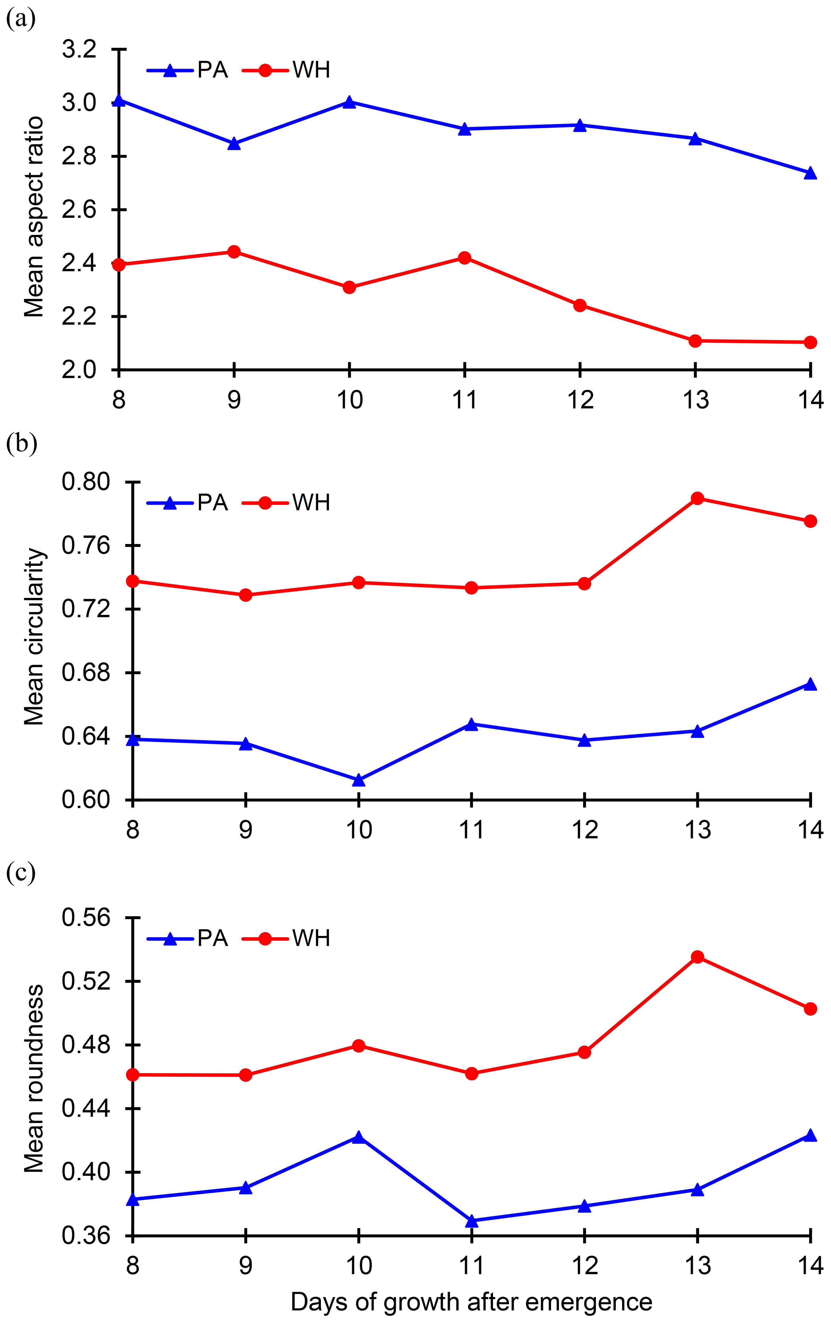
Figure 4. Plot of the (A) mean aspect ratio, (B) mean circularity, and (C) mean roundness of the weed leaves over the second week of growth of Palmer amaranth (PA) and waterhemp (WH).

Figure 5

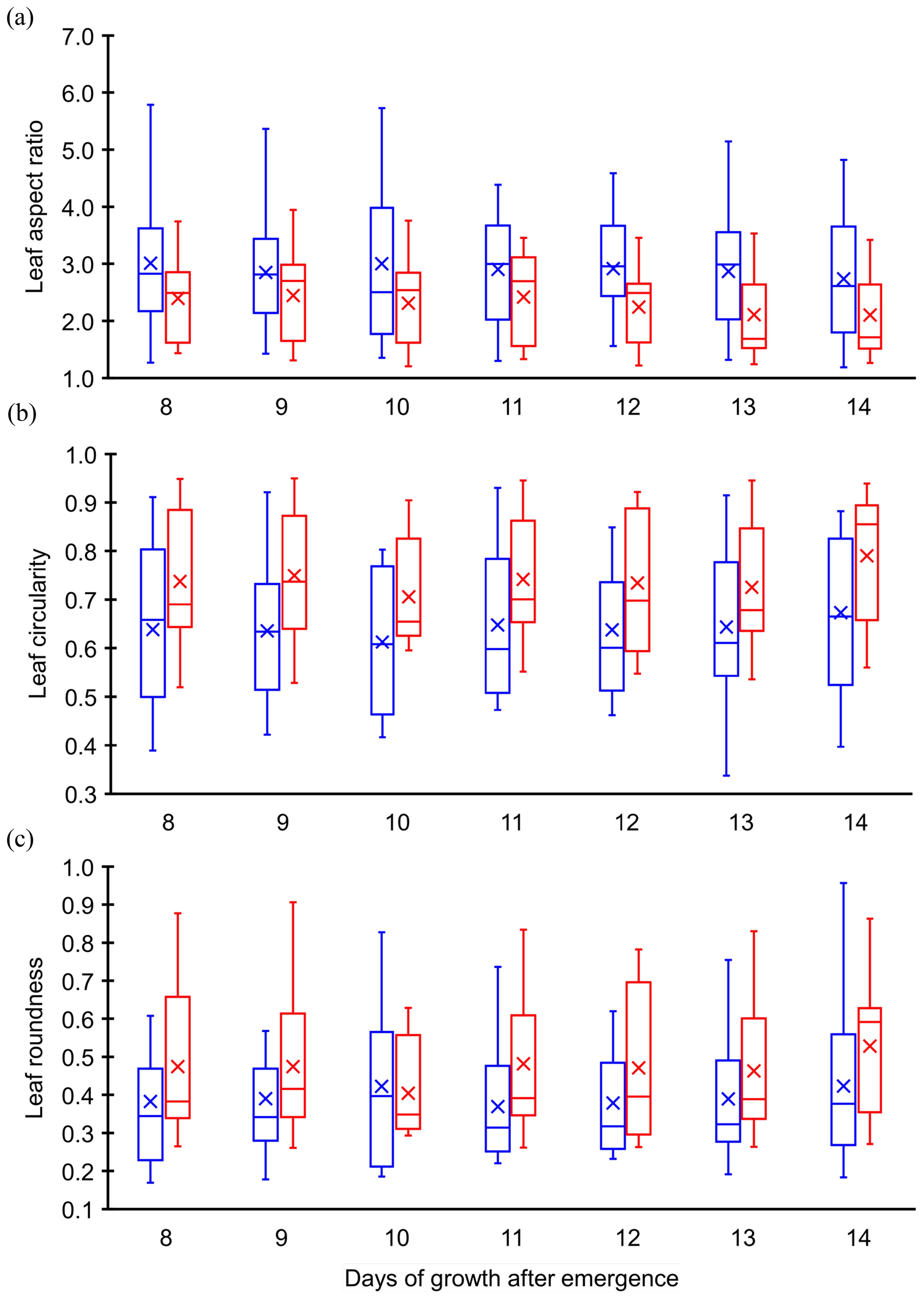
Figure 5. Box plot comparison of leaf (A) aspect ratio, (B) circularity, and (C) roundness. Blue (left) represents Palmer amaranth, and red (right) represents waterhemp.

4.5 Configuration of machine learning classification models

4.5.1 Support vector machine

SVM (Pisner and Schnyer, 2020) is one of the most widely used supervised machine learning algorithms, known for its ability to classify data by constructing hyperplanes that maximize the margin between support vectors. For linearly separable data, a hard margin is applied, while for non-linearly separable data, a soft margin is used. SVM also employs the kernel trick to handle non-linear classification problems. Commonly used kernels include linear, polynomial, radial basis function (RBF), and sigmoid kernels.

In this study, we utilized an SVM with the RBF kernel. Two key hyperparameters in SVM are the penalization parameter (C) and the kernel coefficient (γ). The parameter C controls the trade-off between maximizing the margin and minimizing classification errors by imposing a penalty on misclassifications. A higher value of C results in a model with lower bias and higher variance, meaning it prioritizes minimizing errors but may overfit the data. The parameter γ determines the curvature of the decision boundary by controlling the influence of each data point on the boundary. A higher γ makes the model more sensitive to individual data points, resulting in a more complex decision boundary.

To find the optimal values for C and γ, we employed a grid search with cross-validation (using the ‘GridSearchCV’ technique from the SciPy package). In this process, C was varied logarithmically from 10⁻¹ to 10³ in powers of 10, while γ was varied from 10⁻⁴ to 1. We used fivefold cross-validation to evaluate the performance across different splits of the dataset, optimizing for the most accurate model. As a result of this hyperparameter tuning, the best parameter estimates for C and γ were found to be 100 and 1, respectively.

4.5.2 Random forest classifier

A RF classifier (Probst et al., 2019) is an ensemble learning method that consists of multiple decision tree classifiers, often referred to as estimators. Each estimator is built by randomly sampling a subset of features from the input data, and it classifies the input by casting a vote for a specific class. The final prediction of the RF classifier is determined by aggregating the votes from all individual trees, with the class receiving the majority of votes being selected as the output.

Several hyperparameters influence the performance of the RF classifier. These include the number of estimators, which controls how many decision trees are used; maximum depth, which limits the depth of each tree to prevent overfitting; minimum samples per leaf, which restricts the number of samples required at each leaf node; and minimum samples per split, which controls how many samples are needed to split a node. Additionally, bootstrapping can be applied to introduce variance by sampling subsets of data when building trees.

In our study, we varied these hyperparameters by testing the number of estimators from 10 to 200, maximum depth from 10 to 100, minimum samples per leaf with values of 1, 2, and 4, minimum samples per split with values of 2, 5, and 10, and we considered both bootstrapping and no bootstrapping. To efficiently search for the best hyperparameters, we used a randomized search technique with 100 iterations and fivefold cross-validation, as implemented in SciPy’s ‘RandomizedSearchCV’. This approach, a more computationally efficient alternative to grid search, helped identify the optimal hyperparameters: 73 estimators, a maximum depth of 50, minimum samples split of 10, a minimum samples leaf of 4, and bootstrapping enabled. These settings resulted in the best model performance for the RF classifier in this study.

4.5.3 K-nearest neighbors approach

KNN approach (Taunk et al., 2019) involves distance functions to find a group of ‘ $k$‘ instances that are closest to the unknown samples. Euclidean, Minkowski, Manhattan, and Cosine are some of the distance functions generally used. In our study, Euclidean distance, a widely used distance function is employed. In KNN, the choice of $k$ directly impacts the model’s bias-variance trade-off. A lower $k$ value results in low bias but high variance, leading to potential overfitting, while a higher $k$ value leads to high bias and low variance, risking underfitting. In this study, we varied the $k$ value from 3 to 30 in steps of 1F and selected the $k$ value of 5 as the one that yielded the best performance on the test set.

4.5.4 Logistic regression

LR (Gladence et al., 2015) models the relationship between the input features and the target variable using the sigmoid function, which maps outputs to probabilities between 0 and 1. The model is trained using maximum likelihood estimation as the loss function. For binary classification, data instances with a predicted probability less than or equal to 0.5 are classified as class 0, while those with a probability greater than 0.5 are classified as class 1. Unlike other models, logistic regression does not require hyperparameter tuning, making it a straightforward and efficient approach for binary classification tasks.

All these four machine learning models were trained with hyperparameters optimization using SciPy 1.7.3 package in the Python environment.

4.6 Classification performance of the trained ML models

The classification accuracies of the employed ML models are compared in Figure 6, and it is evident from the figure that the random forest model achieved the top classification accuracy of 70%. Nevertheless, the classification accuracies of the other three models are not far from the accuracy of the random forest model. The classification accuracies of the ML models are in the range of 64% to 70%. Figure 3B shows confusion matrices obtained for the four ML models. Confusion matrices of all the ML models except SVM show that the number of misclassifications of PA instances (to WH) is higher than the number of misclassifications of WH instances (to PA). Consequently, the number of correctly classified PA instances is less than the number of correctly classified WH instances in the confusion matrices of those models. Interestingly, even though misclassifications of both PA and WH are higher in SVM than the other three models, it is the only model where misclassification of PA and WH are almost equal or balanced. The precision of PA and WH for the ML models are plotted in Figure 7A, recall values are plotted in Figure 7B and F₁-score values are plotted in Figure 7C. Precision of PA (0.81) is greatest for the Random Forest model. The precision of WH is almost the same in all the models (0.63-0.65) and it is lower than the Precision of PA in all the models except for the SVM model. Recall of PA is highest (0.66) for the SVM model and Recall of WH is highest (0.88) for the random forest model. The F₁-score of PA is highest (0.64) for the SVM model and the F₁-score of WH is highest (0.75) for the random forest model. The random forest model either outperforms the other three models or performs marginally better than them in most cases. It only performs the poorest in the case of Recall of PA (0.53).

Figure 6

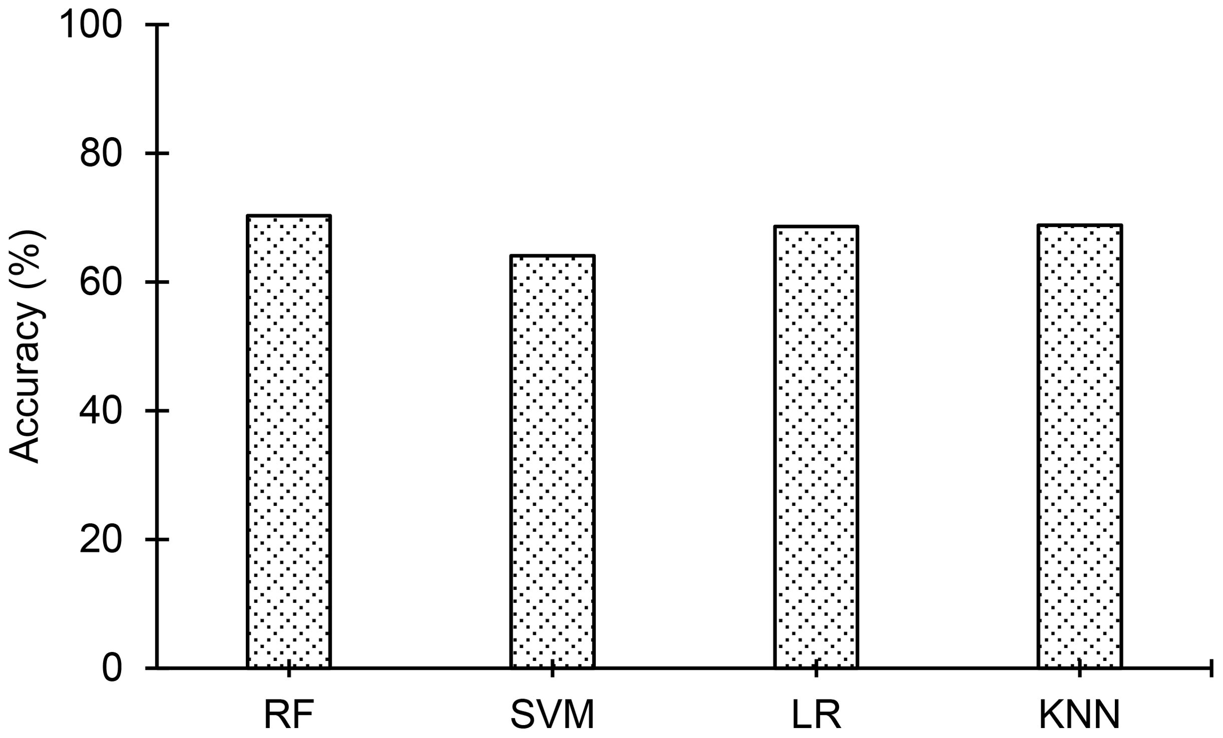
Figure 6. Comparison of classification accuracies of the ML models: 1. Random Forest (RF), 2. Support Vector Machine (SVM), 3. Logistic Regression (LR), and 4. K-nearest neighbors (KNN) employed in the study. The random forest model achieves the top classification accuracy of 70.3% among the ML models.

Figure 7

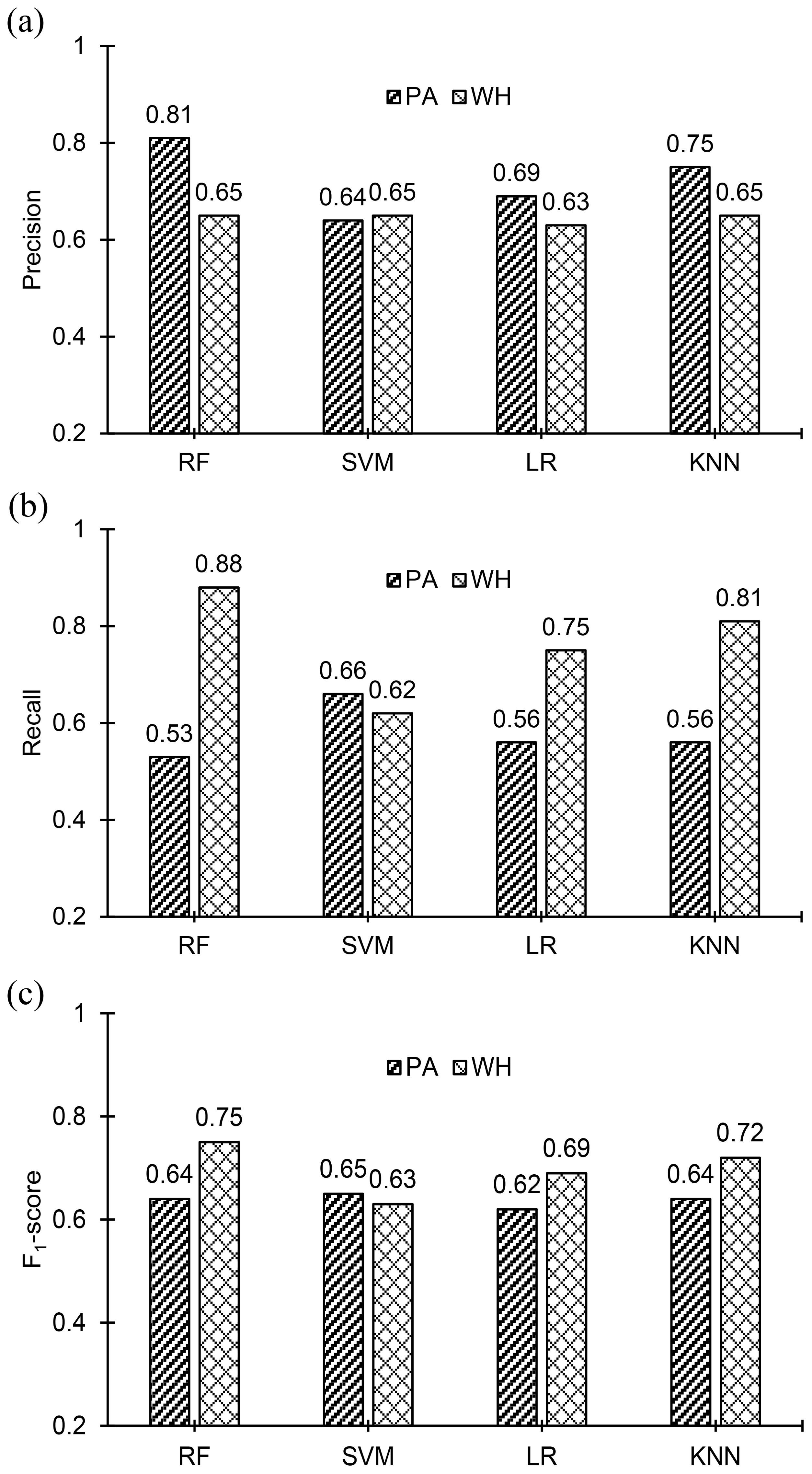
Figure 7. Comparison of (A) precision, (B) recall, and (C) F₁-scores of Palmer amaranth (PA) and waterhemp (WH) for the employed ML models. The random forest model has the highest values of precision for both PA and WH. The highest value of recall of PA and WH is 0.66, for the SVM model, and 0.88, for the random forest model respectively. The F₁-score of PA is almost the same for all the models and the highest value is 0.65 for SVM. The highest F₁-score of WH is 0.75 for the random forest model.

5 Classification of Palmer amaranth and waterhemp using a deep learning approach

The performance of the ML models discussed in the previous section (Section 5) clearly illustrates the inadequacy of the ML approach in satisfactorily distinguishing palmer amaranth from waterhemp. Moreover, the process of hand-crafting the features that are extracting the morphological characteristics and engineering them for further classification by ML models is labor-intensive and time-consuming. Alternatively, Palmer amaranth and waterhemp can be classified directly from their images using a convolutional neural network (CNN), a deep learning model, without the need to extract their leaf geometrical features. Deep learning, a subset of machine learning, is preferred when the input (images, texts, and other media input formats) or the model relationship is too complex to be handled by standard ML approaches (Dargan et al., 2020).

5.1 Background: Working of a CNN

CNN is an artificial neural network extensively used for image-related tasks, notably for image classification. A standard CNN consists of convolutional and pooling layers in addition to fully connected layers. Convolution and pooling layers form the backbone (lower and intermediate layers) of a CNN network and fully connected layers form the head of the network (upper layers). The final layer of the CNN head is the output layer. Convolution layers extract spatially related features from the input image. Convolution involves matrix operations between input and kernel filters and results in feature maps. These feature maps are further transformed with activation functions to impart more non-linearity to the model. ReLU, tanH, and eLU are some commonly used activation functions. Activated feature maps of a convolutional layer or a convolutional block (a stack of convolutional layers) are normally subjected to pooling before subsequent convolution. Pooling decreases the spatial size of the convoluted feature by combining the output of one layer’s neuron cluster into a single neuron in the following layer. Pooling is of two types: max pooling and average pooling. The pooling operation involves sliding a window over feature maps and extracting only the highest (max pooling) or average (average pooling) values of the feature maps bounded by the window as illustrated in Figure 8. The high-level features obtained through successive convolution and pooling operations are feed forwarded further to a fully connected output layer. In the case of image classification, a ‘SoftMax’ activation function is used for the output layer to predict the hot-coded actual output, and a cross-entropy loss function is used for model training. Batch normalization and Dropout layers are also used in CNN for regularizing (generalizing) the network. The batch normalization layer normalizes the input batches of the intermediate layers (Bjorck et al., 2018) and Dropout layers blocks a specified fraction of randomly selected neurons from the training (Baldi and Sadowski, 2013). A regularized network exhibits similar prediction performances for both the exposed data and unforeseen data.

Figure 8

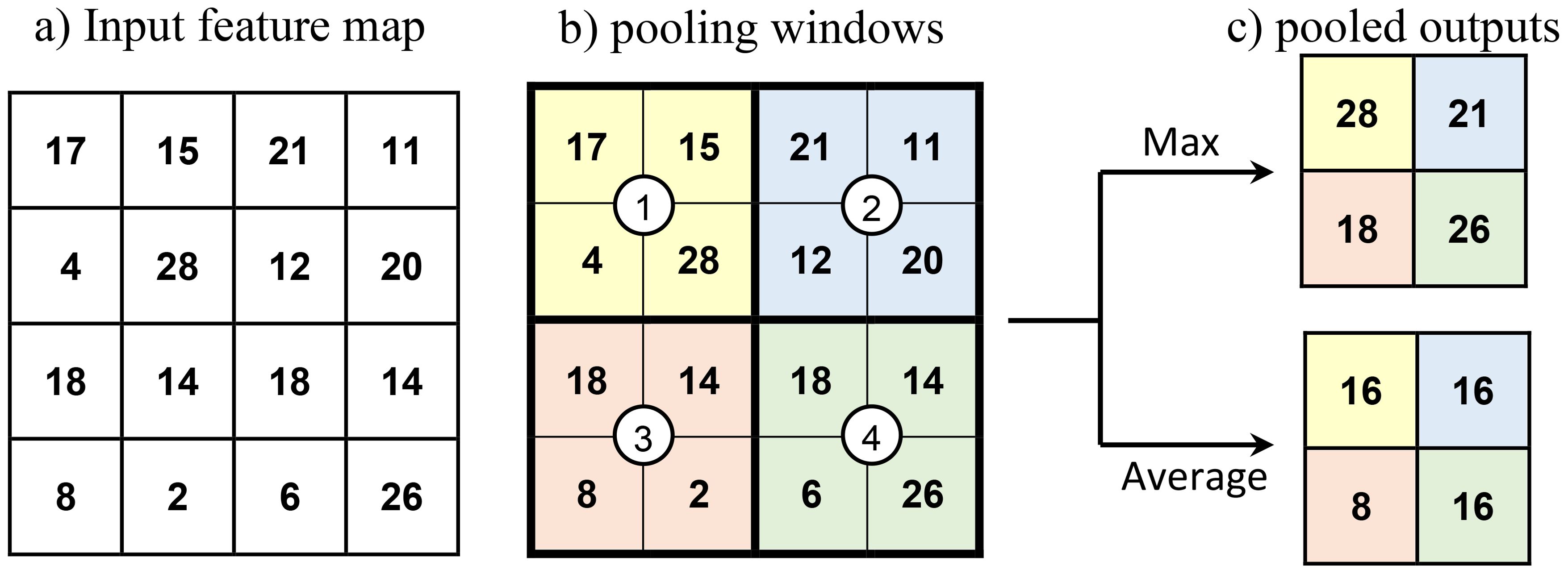
Figure 8. Illustration of pooling operations. (A) A feature map of size 4×4 subject to pooling operations, (B) a pooling window of size 2×2 with stride (step size) of 2 is moved over the input at each step and the encircled numbers show the step position of the center of pooling windows. The color shades indicate the regions involved in the pooling operation at a particular step, and (C) pooled outputs of the input feature map after max pooling and average pooling.

5.2 Dataset preparation for CNN

An image dataset is built from the acquired images of palmer amaranth and waterhemp to train and configure the CNN model. The process of acquiring the image data is described in detail in Section 3. The acquired images are cropped and resized to 200×200 pixels to obtain a leaner model (model with fewer trainable network parameters). A total of 2,000 images, 1000 images for each weed species, are acquired originally. However, to prevent the model from overfitting, 7000 images are added to each weed species through data augmentation techniques which include the change in brightness, change in contrast, conversion to black and white, scaling, and rotation of the original images. Table 5 shows the effect of each augmentation technique used in this analysis on an image example. The final training dataset consists of 16,000 images of size 200×200 pixels in two classes (PA and WH) with 8,000 images per class. The final augmented dataset ($D_2$) for this classification task is comprised of an image array, $X_2\in {ℝ}^{n\times I\times I}$, and a hot-coded label array, $Y_2\in {ℝ}^{n\times c}$ where $n$ is the number of image instances, $I$ is the image dimension, and $c$ is the number of classes which are 18,000, 200, and 2, respectively, for the current task. The dataset used for the training and testing is denoted as $D_{2,tn}$ and $D_{2,tt}$, respectively. The testing dataset, $D_{2,tt}$, consists of 2,000 image instances which are added with gaussian noise of intensity 0.04. This is done to obtain a robust model which does not result in significant degradation of classification performance for the field images addled with noises. Figure 9 shows an example image added with the gaussian noise.

Table 5

Table 5. Data augmentation techniques and their effects on an image.

Figure 9

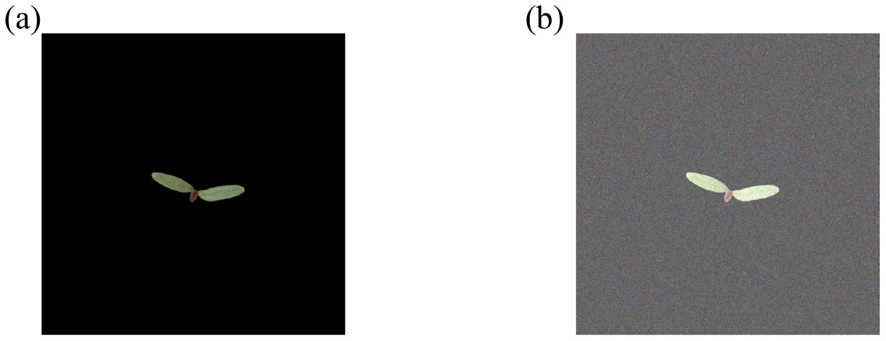
Figure 9. (A) Preprocessed image of weed foliage used in the deep learning classification, and (B) the same image after the addition of Gaussian noise of intensity 0.04.

5.3 Training and configuration of CNN (DL) model

The CNN model is trained and configure using TensorFlow 2.6.2. The model was fitted to the training dataset using ADAM (Kingma and Ba, 2014) optimization with 100 epochs. Several configurations for CNN model were explored by increasing the number of filters and the number of convolutional layers to improve feature extraction capabilities. Additionally, batch normalization was tested to stabilize and accelerate the training process by normalizing the input batches for intermediate layers. To further enhance the generalization performance of the model, we investigated dropout values ranging from 0.1 to 0.5. Based on the classification performance on both the training and testing datasets, a dropout value of 0.2 was selected as the optimal balance between underfitting and overfitting. To prevent overfitting and ensure the best generalization to unseen data, early stopping criteria were applied. This allowed the model to halt training when test accuracy began to drop, effectively selecting the model with the best generalization performance. Dropout layers and early stopping helped ensure that the final model did not overfit, while achieving stable classification performance across training and testing datasets. The architecture of the finally configured CNN model is shown in Figure 10, with the details of its layers summarized in Table 6. The model employed ReLU activation in the convolutional layers and SoftMax in the output layer for classification.

Figure 10

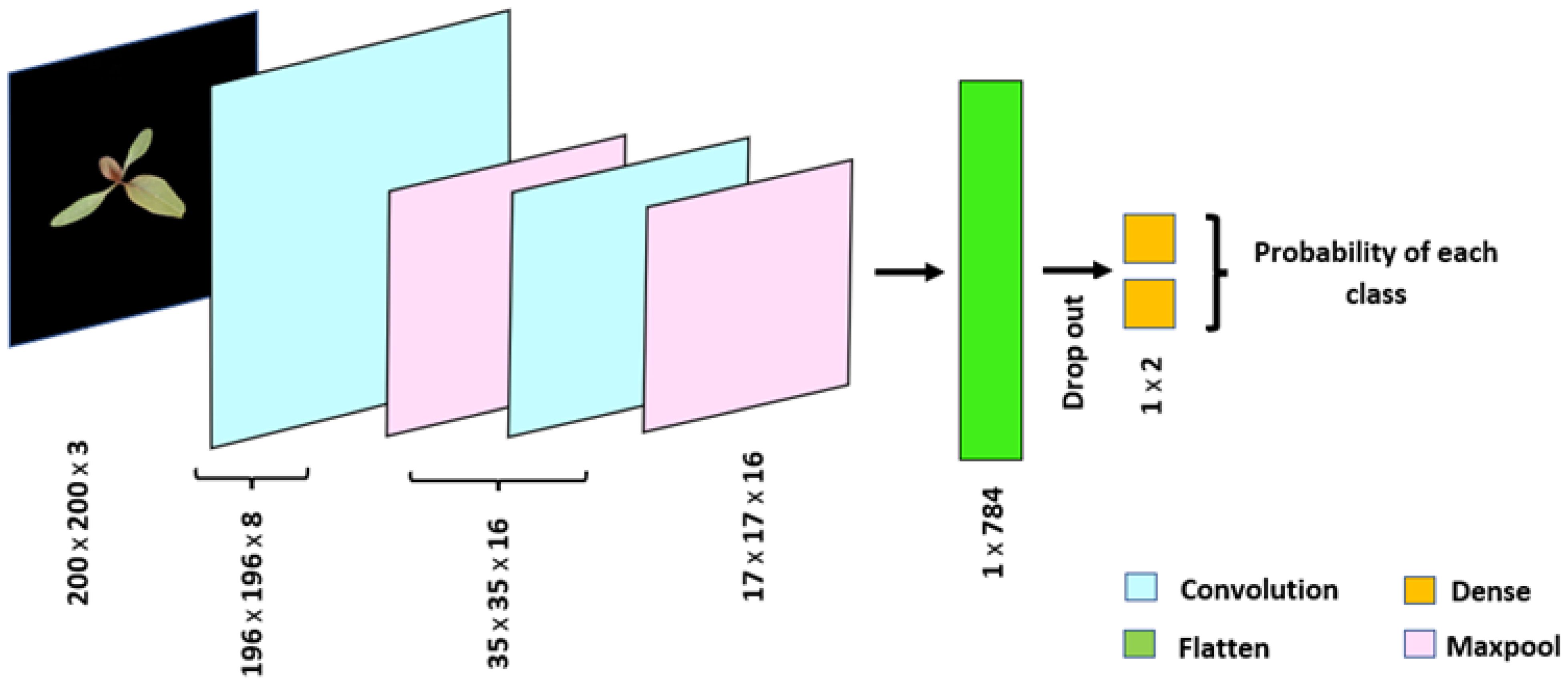
Figure 10. Architecture of convolutional neural network, a deep learning model, employed in the study for the classification of Palmer amaranth and waterhemp. The network consists of 5,394 trainable parameters and achieved a classification accuracy of 92.3% on the Gaussian noise-added testing dataset.

Table 6

Table 6. Details of the convolutional neural network architecture used for the classification of Palmer amaranth and waterhemp.

5.4 Classification performance of the CNN

Classification accuracies of 96.2% and 92.8% are obtained for the training and the testing dataset respectively using the configured model. The small positive difference between the classification accuracies of the training (96.2%) and testing (92.8%) datasets indicates that there is no significant overfitting in the model, suggesting that the model generalizes well to unseen data. The slight discrepancy may be attributed to the inclusion of noisy images in the testing dataset. These noisy images simulate real-world conditions and naturally make classification more challenging, which can lead to a marginal drop in performance compared to the cleaner training data. The classification accuracy (92.8%) obtained for the CNN model (deep learning model) is significantly higher than the accuracy (70.3%) of the random forest model (ML model). Figure 11 shows the confusion matrix of the model for the test data along with the confusion matrix of the random forest model (top ML model). The confusion matrix reveals that the inaccuracy of the model is mainly due to the misclassification of 145 image instances of PA as WH. Accordingly, both the Precision of PA and the Recall of WH are 100%, while the Precision of WH and the Recall of PA are 87% and 85% respectively. F₁-scores of PA and WH are almost equal and of value 92.5% approximately. Class-wise performance metrics namely Precision, Recall, and F₁-score of the CNN model are compared with the performance metrics of the random forest model in Figure 12. As observed in the figures, class-wise performance metrics of the CNN model also outperform the ML model.

Figure 11

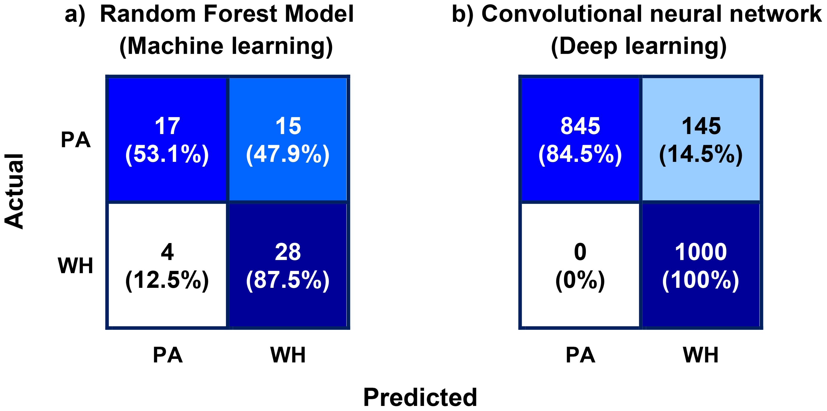
Figure 11. (A) Confusion matrix of the best machine learning model (random forest model) and (B) confusion matrix of the deep learning (DL) model (convolutional neural network, CNN). Each cell of the confusion matrices shows the total number of instances (top), and the percentage of class instances (bottom) that belong to the respective cell categories. The misclassification of Palmer amaranth (PA) instances as waterhemp (WH) is significantly higher than the misclassification of WH as PA, both in the case of the ML model and the DL model.

Figure 12

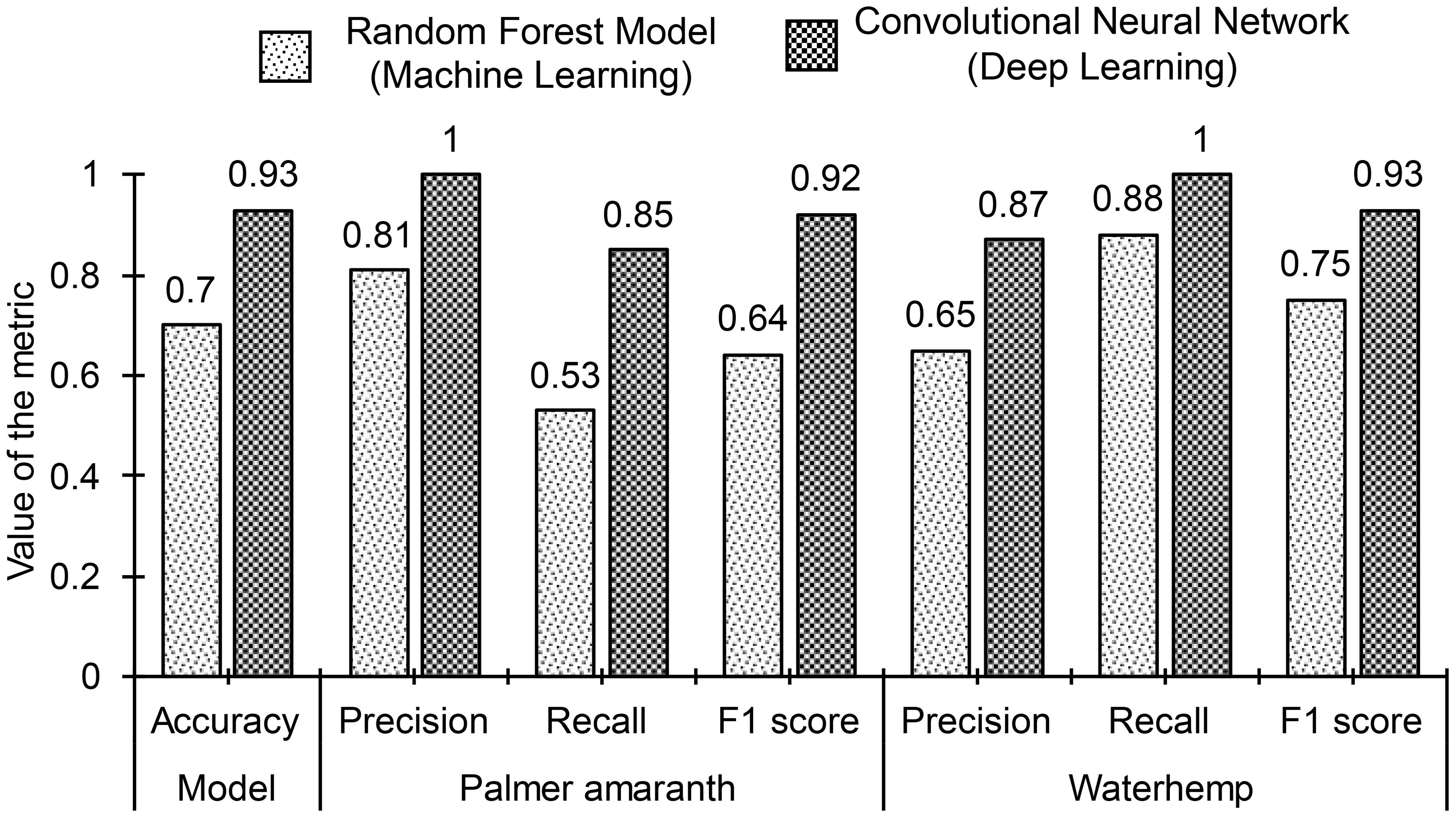
Figure 12. Comparison of classification performance of the top machine learning model (random forest model) and the deep learning model (convolutional neural network). The deep learning model outperforms the top machine learning model on all fronts of performance evaluations.

6 Multi-object classification of mixture of weed foliage using transfer learning

In Section 6, a highly accurate CNN model is designed for the classification of Palmer amaranth and waterhemp. Though the model is accurate, it can only identify whether the given image belongs to either Palmer amaranth or waterhemp and it requires single object input images. Here, a single object means single foliage of either of the weed plants. However, the real-time identification of these two weed species will involve field images that contain a random mixture of foliage of both weed species. Thus, it is important to localize each object (foliage of either weed species) which means identifying individual objects in an image and categorizing it to either of the classes. This necessitates the need for an object detection model for accurate localization of the weed foliage.

6.1 Background: object detection (multi-object classification)

Object detection is a computer vision technique that locates individual objects by drawing bounding boxes around the objects and labeling them according to their classes (Zou et al., 2019). The process of object detection involves three stages: 1. informative region selection in which the input images are scanned through a multiscale sliding window to find all the possible regions of objects 2. feature selection where visual features of the objects in the image are extracted for object recognition, and 3. classification in which each object is labeled according to their classes. Training an accurate object detection model from the ground up requires a fully annotated image dataset of large size which comprise different combinations of individual objects. Building such large datasets is usually highly expensive and not viable in many cases. However, object detection models of the desired accuracy can be designed with smaller datasets using transfer learning (Jose et al., 2022). Transfer learning (Zhuang et al., 2021), an ML method, adopts the knowledge acquired in a different but similar task to improve the learning of the current task. Transfer learning is formally defined using two important definitions namely ‘domain’ and ‘task’. Domain, $\mathcal{D}$, is characterized by a feature space, $\mathcal{F}$, and a marginal distribution, $\text{P}\left(\text{X}\right)$, where $\text{X }\left(\in \mathcal{F}\right)$ is the feature data and $\mathcal{F}$ spans all the possible feature data. Task, $\mathcal{T}$, is characterized by a label space, $\mathcal{L}$, and a conditional distribution, $\text{P}\left(\text{Y}|\text{X}\right)$, where $\text{Y }\left(\in \mathcal{T}\right)$ is the label data and $\mathcal{L}$ spans all the possible label data. Formally, transfer learning focuses on learning the task, ${\mathcal{T}}_T$, in the target domain, ${\mathcal{D}}_{\text{T}}$, by utilizing the knowledge of the task, ${\mathcal{T}}_{\text{S}}$, executed in the source domain, ${\mathcal{D}}_{\text{S}}$. The subscript $S$ and $T$ stands for the source and the target respectively. Transfer learning for object detection is executed with the following three steps, 1. identifying a well-trained object detection model with a feature space that can accommodate our feature data (multi-object weed images), 2. modifying the head of the object detection model by adding a few trainable layers including the output layer to rework the label space, and 3. fine tune the trainable layers to carry out the target task (detection of the weed species).

6.2 Dataset preparation

An annotated image dataset is built to fine-tune the head of the object detection model. The annotation of the images used in the dataset involves drawing bounding boxes around objects (weed foliage) in the images and obtaining the objects’ classes, coordinates, and dimensions of the bounding boxes. A total of 3,200 images, 1,600 per each weed class, are used for the training dataset and the annotation for these images is carried out using an open-source tool called ‘LabelImg’. All these images contain only one object (foliage of either of a weed classes). Thus, the training dataset, $D_{3,tn}$, built for the object detection task consisting of an image array, $X_{3,tn}\in {ℝ}^{n\times I\times I},$ and an annotation array, $Y_{3,tn}\in {ℝ}^{n\times p}$. Here, $n$, the number of instances, is 3,200, and $p$, the number of annotation columns, is 5. A $k$th row of the annotation array is defined as $y_k=\left(l,x,y,b,h\right)$, where $l$ is an object label, $x$ and $y$ are coordinates of a bounding box, and $b$ and $h$ are width and height of a bounding box, respectively. To test the performance of the trained object detection model, a testing dataset, $D_{3,tn}$, consisting of 12 multi-object (more than one object in an image) images of size 4,000 × 4,000 is constructed. The multi-object images are created by making collages of 10 to 12 weed foliages of palmer amaranth and waterhemp on a black background. The foliages of the weed plants are randomly selected from 132 weed images (61 per each class) that were not part of the $D_{3,tn}$. To simulate the field setting, the weed foliages in a multi-object image are chosen with different ages and are spread around randomly both at close and distant proximities. Figure 13 shows two examples of the multi-object images created for testing the object detection model, and Figure 14 shows the labeled image outputs of the trained object detection model for the image examples shown in Figure 13. The bounding boxes in red color represent palmer amaranth class and the pink color bounding boxes represent waterhemp class.

Figure 13

Figure 13. Multi-object images developed for the training of the object detection model. These images are generated by distributing the individual foliages of (A) Palmer amaranth and (B) waterhemp over a black background.

Figure 14

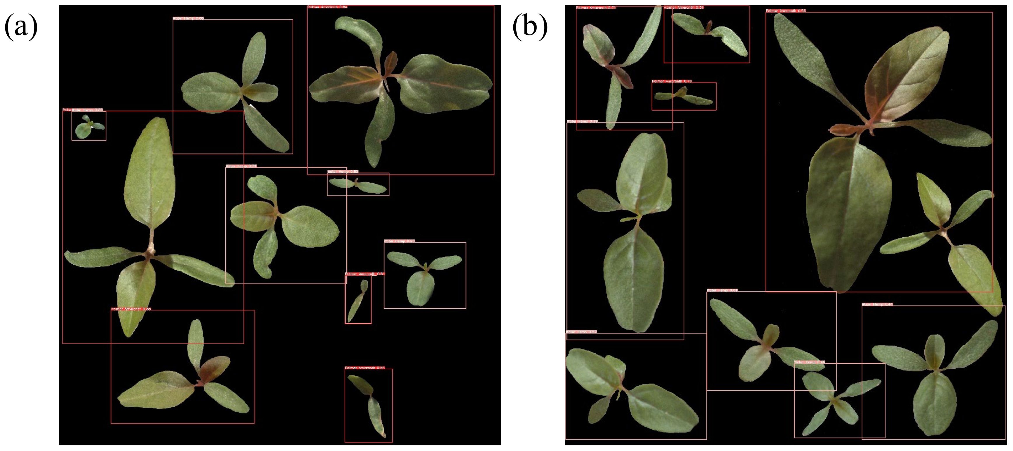
Figure 14. Multi-object images predicted with class labels and confidence scores by the fine-tuned YOLOv5 model. The red and pink bounding boxes denote (A) Palmer amaranth and (B) waterhemp, respectively.

6.3 Configuration of an object detection model

In this study, a state-of-the-art object detection model, YOLOv5, pre-trained on the COCO dataset is employed for weed detection. YOLOv5, an acronym for You Only Look Once, is a powerful single-stage object detector that detects objects present in an image in a single shot. Single-stage object detectors, though slightly less accurate, are faster than two-stage object detectors. Single-stage object detectors make predictions directly from the generated feature maps whereas two-stage detectors employ a region proposal network for processing the feature maps and making predictions on the proposed regions. The YOLOv5 model is composed of three network components, a backbone, a neck, and a head. The backbone of YOLOv5 uses cross stage partial (CSP) network for extracting information-rich features from the image. It also decreases the image resolution and enhances its feature resolution. The neck is composed of spatial pyramid pooling (SPP) and path aggregation network (PANet) and is responsible for constructing feature pyramids. Feature pyramids are important for scale invariance and generalizing performance of the object detection model. Finally, the head which consists of three convolutional layers predicts the location and size of the bounding boxes, object scores, and object classes. More about YOLOv5 can be read elsewhere (Thuan, 2021). The COCO dataset (Lin et al., 2014) used for pretraining YOLOv5 consists of 330,000 images of 80 different general object categories (dog, cat, boat, airplane, plants, and so on). The final three convolution layers of the YOLOv5 are configured to label the object into two weed classes: PA and WH.

6.4 Object detection (multi-object classification) model performance

The results of the object detection model obtained for the 12 test images are summarized in Table 7. Figures 15, 16 show the graphical comparison of the classification accuracies of PA, WH, and both PA and WH for the test images. As observed in Figure 15, 75% of the test images are predicted with object detection accuracies of 80% and above and the mean object detection accuracy of the model is 84.8% with a standard error of 3.53% (refer Figure 17). It is evident from these results that the model achieves consistently good accuracies for most of the test images. The mean accuracies of the model for Palmer amaranth and waterhemp are 85.3% and 82.8%, respectively, and the standard errors are 2.95% and 5.63%, respectively. This shows that the model identifies palmer amaranth more accurately and consistently than waterhemp. However, the model has shown satisfactory performance overall in identifying the weed foliages irrespective of their age and proximity to each other and thus will be a useful model in a real field setting.

Table 7

Table 7. Summary of the object detection results obtained for the test images.

Figure 15

Figure 15. Summary of the object detection accuracies of the test images for Palmer amaranth (PA) and waterhemp (WH). The accuracies for both PA and WH are above 80% for most images.

Figure 16

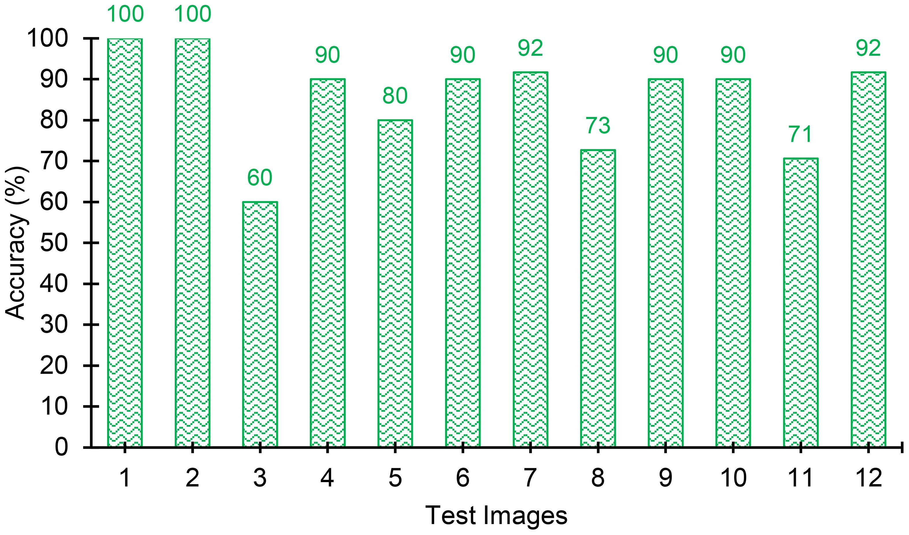
Figure 16. Combined accuracies (including both Palmer amaranth and waterhemp) of the test images. The model achieves consistently good accuracies for most of the test images.

Figure 17

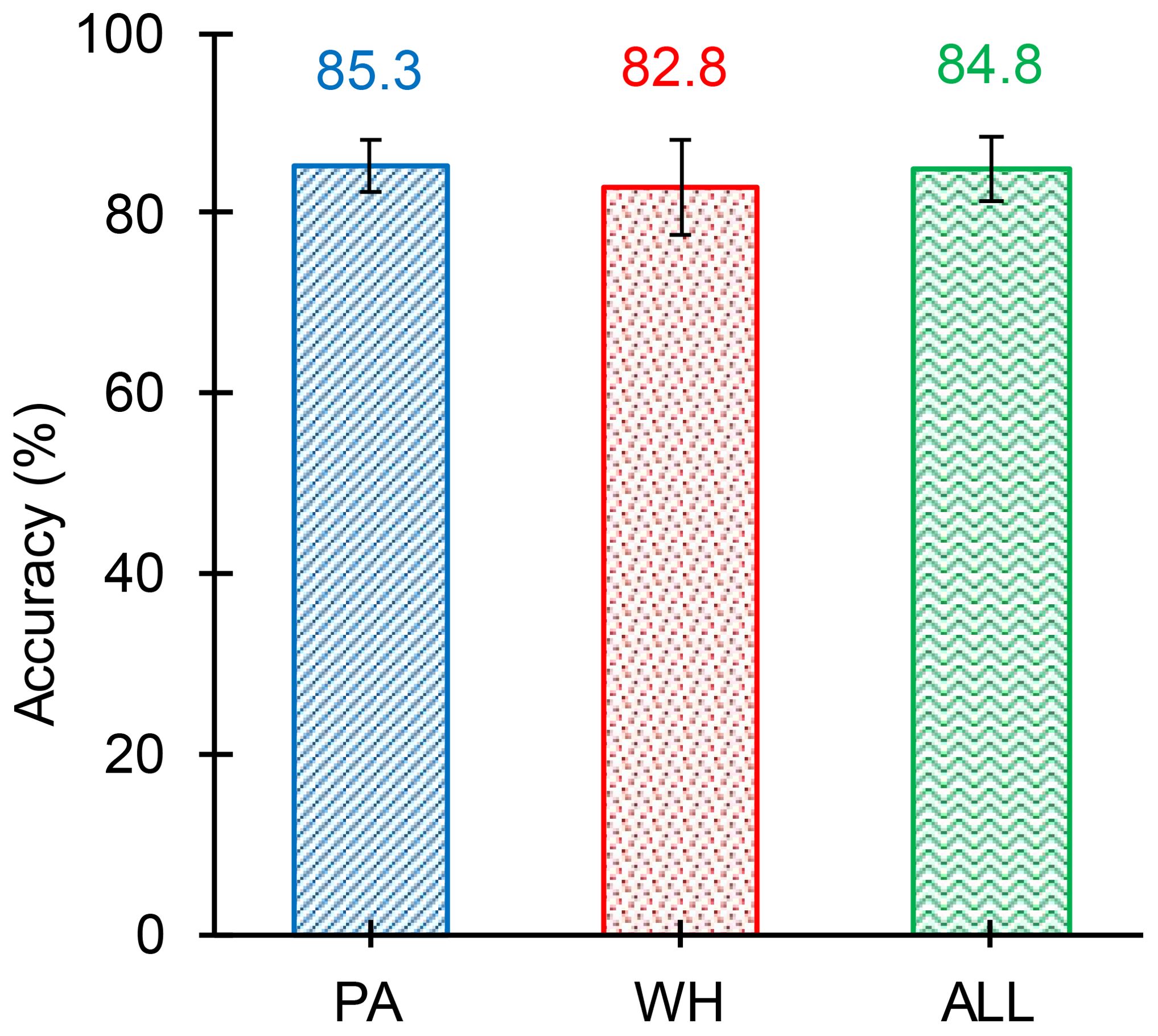
Figure 17. Mean objection detection accuracy (averaged over all the test images) of the model for Palmer amaranth (PA), waterhemp (WH), and both PA and WH (ALL). The mean accuracy of WH is slightly lesser than PA, however, the difference observed is marginal. The variability of WH (Standard Error - 5.63) is greater than the variability of PA (Standard Error - 2.95). The overall object detection accuracy of the model is 84.8% with a standard error of 3.43%.

7 Conclusions

The purpose of the current study is to automate the detection of Palmer amaranth and waterhemp in the early stages of growth (within two weeks of growth after germination). To this end, three different AI approaches namely machine learning, deep learning, and objection detection were employed for weed detection. The outcomes and conclusions drawn from the analysis conducted in the study and from the implementation of these approaches are summarized below:

1. The dimensionless leaf parameters such as aspect ratio, circularity, and roundness generally used for differentiating fully grown Palmer amaranth and waterhemp can only be measured in the second week after emergence (Day 8 to Day 14) because of the lack of visible growth in the first week. The distribution of these dimensionless parameters of Palmer amaranth and waterhemp in the second week of growth have shown a significant and complex overlap between them.

2. Four top-performing ML models namely random forest, SVM, logistic regression, and KNN were employed to classify Palmer amaranth and waterhemp. Random forest, being the top-performing ML model, achieved a classification accuracy of 70%. The F₁ scores of Palmer amaranth and waterhemp for the random forest model were 0.64 and 0.75, respectively. Though the classification performance of the ML approach is not satisfactory, the ML models only involved a small amount of data (312 data instances with 156 data instances per class) for the model training. However, the extraction of the dimensionless features for a such small amount of data is time-consuming and requires manual intervention.

3. A convolutional neural network employed as a deep learning model resulted in a good classification accuracy of 93.2%. The F₁ scores of Palmer amaranth and waterhemp for the random forest model were 0.92 and 0.93, respectively. The deep learning approach required a larger amount of data compared to the ML approach and hence the original data size of 4000 (2000 image instances per class) is increased to 16,000 (8,000 image instances per class) using data augmentation techniques. Though the DL approach is data-intense, it performed significantly better than the best ML model.

4. The object detection model for the localized identification of weeds from the images mixed with foliages of Palmer amaranth and waterhemp was developed with the use of transfer learning. By fine-tuning the head of YOLOv5 (the top 3 convolutional layers) trained on the COCO dataset, an average object detection accuracy of 83.5% is achieved. Only 3,200 single-object images (images with single foliage of either palmer amaranth or waterhemp) are used for fine-tuning. The developed object detection model can identify the weed foliages irrespective of their age and proximity to each other and thus will be a useful model in a real field setting.

8 Limitations and future research

The images used in the classification and identification of Palmer amaranth and waterhemp were captured under a laboratory setting with controlled lighting conditions and with a simple background. The effectiveness of these automation approaches for the images acquired with different incident angles, inclusions of plant and other extraneous features, different environmental conditions, and different lighting conditions need to be studied since the performance of the machine learning and deep learning models was influenced by the process of image acquisition. Even though it is evident that the early distinguishing of Palmer amaranth from waterhemp is valuable for weed management and consequently for enhancing crop yields, cost analysis quantifying the financial impacts will be beneficial to the agricultural community. The study currently distinguishes Palmer amaranth from waterhemp, but it can be extended to distinguishing Palmer amaranth from the other pigweed species namely redroot pigweed (Amaranthus retroflexus), smooth pigweed (Amaranthus hybridus), and Powell amaranth (Amaranthus powellii).

Data availability statement

The original contributions presented in the study are included in the article/supplementary material. Further inquiries can be directed to the corresponding author.

Author contributions

AV: Data curation, Formal analysis, Investigation, Writing – original draft, Writing – review & editing. DA: Formal analysis, Methodology, Visualization, Writing – original draft, Writing – review & editing. RY: Conceptualization, Funding acquisition, Methodology, Project administration, Supervision, Writing – original draft, Writing – review & editing. TP: Investigation, Resources, Supervision, Writing – review & editing.

Funding

The author(s) declare financial support was received for the research, authorship, and/or publication of this article. This study was supported by North Dakota Corn Utilization Council. Any opinions, findings, conclusions, or recommendations provided in this paper are those of the author(s) and do not necessarily reflect the views of the funding agency.

Acknowledgments

The corresponding author gratefully acknowledges Prof. Amit Jhala from University of Nebraska-Lincoln for providing the Palmer amaranth and waterhemp seeds used for conducting this study.

Conflict of interest

The authors declare that the research was conducted in the absence of any commercial or financial relationships that could be construed as a potential conflict of interest.

Publisher’s note

All claims expressed in this article are solely those of the authors and do not necessarily represent those of their affiliated organizations, or those of the publisher, the editors and the reviewers. Any product that may be evaluated in this article, or claim that may be made by its manufacturer, is not guaranteed or endorsed by the publisher.

References

Aakif A., Khan M. F. (2015). Automatic classification of plants based on their leaves. Biosyst. Eng. 139, 66–75. doi: 10.1016/j.biosystemseng.2015.08.003

Crossref Full Text | Google Scholar

Baldi P., Sadowski P. J. (2013). Understanding dropout. Adv. Neural Inf. Process. Syst. 26, 2814–2822.

Google Scholar

Bensch C. N., Horak M. J., Peterson D. (2003). Interference of redroot pigweed (Amaranthus retroflexus), Palmer amaranth (A. palmeri), and common waterhemp (A. rudis) in soybean. Weed Sci. 51, 37–43. doi: 10.1614/0043-1745(2003)051[0037:IORPAR]2.0.CO;2

Crossref Full Text | Google Scholar

Berger S. T., Ferrell J. A., Rowland D. L., Webster T. M. (2015). Palmer amaranth (Amaranthus palmeri) competition for water in cotton. Weed Sci. 63, 928–935. doi: 10.1614/WS-D-15-00062.1

Crossref Full Text | Google Scholar

Bjorck N., Gomes C. P., Selman B., Weinberger K. Q. (2018). Understanding batch normalization. Adv. Neural Inf. Process. Syst. 31, 7694–7705.

Google Scholar

Bradley K., Nordby D., Hartzler B. (2022). Biology and management of waterhemp. The Glyphosate, Weeds and Crops Series GWC-13.

Google Scholar

Butts T. R., Vieira B. C., Latorre D. O., Werle R., Kruger G. R. (2018). Competitiveness of herbicide-resistant waterhemp (Amaranthus tuberculatus) with soybean. Weed Sci. 66, 729–737. doi: 10.1017/wsc.2018.45

Crossref Full Text | Google Scholar

Chahal P. S., Aulakh J. S., Jugulam M., Jhala A. J. (2015). “Herbicide-resistant Palmer amaranth (Amaranthus palmeri S. Wats.) in the United States—mechanisms of resistance, impact, and management,” in Herbicides, Agronomic Crops and Weed Biology (InTech, Rijeka, Croatia), 1–29.

Google Scholar

Dargan S., Kumar M., Ayyagari M. R., Kumar G. (2020). A survey of deep learning and its applications: a new paradigm to machine learning. Arch. Comput. Methods Eng. 27, 1071–1092. doi: 10.1007/s11831-019-09344-w

Crossref Full Text | Google Scholar

Elnemr H. A. (2017). “Feature selection for texture-based plant leaves classification,” in 2017 Intl Conf on Advanced Control Circuits Systems (ACCS) Systems & 2017 Intl Conf on New Paradigms in Electronics & Information Technology (PEIT), Alexandria, Egypt. (New York: IEEE), 91–97. doi: 10.1109/ACCS-PEIT.2017.8303025

Crossref Full Text | Google Scholar

Gladence L. M., Karthi M., Anu V. M. (2015). A statistical comparison of logistic regression and different Bayes classification methods for machine learning. ARPN J. Eng. Appl. Sci. 10, 5947–5953.

Google Scholar

Heap I. (2020). The international herbicide-resistant weed database. Available at: http://www.weedscience.org/Home.aspx

Google Scholar

Ikley J., Jenks B. (2019). Identification, Biology and Control of Palmer Amaranth and Waterhemp in North Dakota (Fargo: NDSU Extension, North Dakota State University).

Google Scholar

Jiang H., Köhler C. (2012). Evolution, function, and regulation of genomic imprinting in plant seed development. J. Exp. Bot. 63, 4713–4722. doi: 10.1093/jxb/ers145

PubMed Abstract | Crossref Full Text | Google Scholar

Jose J. A., Sharma A., Sebastian M., Densil R. V. F. (2022). “Classification of Weeds and crops using transfer learning,” in 2022 International Conference on Advances in Computing, Communication and Applied Informatics (ACCAI) (New York: IEEE), 1–7.

Google Scholar

Kingma D. P., Ba J. (2014). Adam: A method for stochastic optimization. arXiv preprint arXiv:1412.6980. doi: 10.48550/arXiv.1412.6980

Crossref Full Text | Google Scholar

Kohrt J. R., Sprague C. L. (2017). Herbicide management strategies in field corn for a three-way herbicide-resistant Palmer amaranth (Amaranthus palmeri) population. Weed Technol. 31, 364–372. doi: 10.1017/wet.2017.18

Crossref Full Text | Google Scholar

Lin T.-Y., Maire M., Belongie S., Hays J., Perona P., Ramanan D., et al. (2014). “Microsoft coco: Common objects in context,” in Computer Vision–ECCV 2014: 13th European Conference, Zurich, Switzerland, Proceedings, Part V 13 (Springer International Publishing), 740–755.

Google Scholar

Mahesh B. (2020). Machine learning algorithms-a review. Int. J. Sci. Res. (IJSR). 9, 381–386. doi: 10.21275/ART20203995

Crossref Full Text | Google Scholar

Mahoney D. J., Jordan D. L., Hare A. T., Leon R. G., Roma-Burgos N., Vann M. C., et al. (2021). Palmer amaranth (Amaranthus palmeri) growth and seed production when in competition with peanut and other crops in North Carolina. Agronomy 11, 1734. doi: 10.3390/agronomy11091734

Crossref Full Text | Google Scholar

Massinga R. A., Currie R. S., Horak M. J., Boyer J. (2001). Interference of Palmer amaranth in corn. Weed Sci. 49, 202–208. doi: 10.1614/0043-1745(2001)049[0202:IOPAIC]2.0.CO;2

Crossref Full Text | Google Scholar

Molin W. T., Nandula V. K. (2017). Morphological Characterization of Amaranthus palmeri x A. spinosus Hybrids. Am. J. Plant Sci. 8, 1499–1510. doi: 10.4236/ajps.2017.86103

Crossref Full Text | Google Scholar

Montgomery J. S., Sadeque A., Giacomini D. A., Brown P. J., Tranel P. J. (2019). Sex-specific markers for waterhemp (Amaranthus tuberculatus) and Palmer amaranth (Amaranthus palmeri). Weed Sci. 67, 412–418. doi: 10.1017/wsc.2019.27

Crossref Full Text | Google Scholar

Naser M., Alavi A. H. (2021). Error metrics and performance fitness indicators for artificial intelligence and machine learning in engineering and sciences. Archit. Struct. Constr. 3, 499–517. doi: 10.1007/s44150-021-00015-8

Crossref Full Text | Google Scholar

Perkins C. M., Gage K. L., Norsworthy J. K., Young B. G., Bradley K. W., Bish M. D., et al. (2021). Efficacy of residual herbicides influenced by cover-crop residue for control of Amaranthus palmeri and A. tuberculatus in soybean. Weed Technol. 35, 77–81. doi: 10.1017/wet.2020.77

Crossref Full Text | Google Scholar

Pisner D. A., Schnyer D. M. (2020). “Support vector machine.” in Machine learning (Cambridge, Massachusetts: Academic Press), 101–121. doi: 10.1016/B978-0-12-815739-8.00006-7

Crossref Full Text | Google Scholar

Probst P., Wright M. N., Boulesteix A. L. (2019). Hyperparameters and tuning strategies for random forest. Wiley Interdiscip. Reviews: Data Min. knowledge Discovery 9, e1301. doi: 10.1002/widm.1301

Crossref Full Text | Google Scholar

Roberts J., Florentine S. (2022). A review of the biology, distribution patterns and management of the invasive species Amaranthus palmeri S. Watson (Palmer amaranth): Current and future management challenges. Weed Res. 62, 113–122. doi: 10.1111/wre.12520

Crossref Full Text | Google Scholar

Salve P., Sardesai M., Manza R., Yannawar P. (2016). “Identification of the plants based on leaf shape descriptors,” in Proceedings of the Second International Conference on Computer and Communication Technologies: IC3T 2015, vol. 1. (India: Springer), 85–101.

Google Scholar

Steckel L. E., Sprague C. L. (2004). Common waterhemp (Amaranthus rudis) interference in corn. Weed Sci. 52, 359–364. doi: 10.1614/WS-03-066R1

Crossref Full Text | Google Scholar

Taunk K., De S., Verma S., Swetapadma A. (2019). “A brief review of nearest neighbor algorithm for learning and classification,” in 2019 International Conference on Intelligent Computing and Control Systems (ICCS) (India: IEEE), 1255–1260.

Google Scholar

Thuan D. (2021). Evolution of Yolo algorithm and Yolov5: The State-of-the-Art object detention algorithm. Thesis.

Google Scholar

Trucco F., Tatum T., Robertson K. R., Rayburn A. L., Tranel P. J. (2006). Characterization of waterhemp (Amaranthus tuberculatus)× smooth pigweed (A. hybridus) F1 hybrids. Weed Technol. 20, 14–22. doi: 10.1614/WT-05-018R.1

Crossref Full Text | Google Scholar

Zhuang F., Qi Z., Duan K., Xi D., Zhu Y., Zhu H., et al. (2021). A comprehensive survey on transfer learning. Proc. IEEE 109, 43–76. doi: 10.1109/JPROC.2020.3004555

Crossref Full Text | Google Scholar

Zou Z., Shi Z., Guo Y., Ye J. (2019). Object detection in 20 years: A survey. arXiv preprint arXiv:1905.05055. doi: 10.48550/arXiv.1905.05055

Crossref Full Text | Google Scholar